Probability analysis of undrained clay slope stability considering strength anisotropy and heterogeneous rotated anisotropy

Strength anisotropy and heterogeneous rotated anisotropy are prevalent phenomena in natural slopes. Previous studies have underscored their significance in slope stability analysis. However, in previous slope stability analyses, the effects of strength anisotropy and heterogeneous rotated anisotropy on slope stability were studied separately, without considering their coupled effect. This paper aims to propose a probabilistic analysis framework of slope stability considering the coupled effect of strength anisotropy and heterogeneous rotated anisotropy. Through an undrained clay slope case, the proposed probabilistic analysis framework is examined. The influence of strength anisotropy and heterogeneous rotated anisotropy on slope stability is investigated. The results show that the proposed probabilistic analysis framework of slope stability considering the coupled effect of strength anisotropy and heterogeneous rotated anisotropy is effective. Both strength anisotropy and heterogeneous rotated anisotropy have an important influence on slope stability. Furthermore, the statistics of safety factor including mean value, coefficient of variation, and reliability index, vary with the strength anisotropy coefficient, the heterogeneous anisotropy coefficient, and the rotational angle. The smaller the strength anisotropy coefficient, the larger the heterogeneous anisotropy coefficient, and the smaller the reliability index. The rotational angle of strata corresponding to the minimum and maximum values of the slope reliability index is sensitive to the strength anisotropy coefficient, but not to the heterogeneous anisotropy coefficient.

1 Introduction

The soil layers in nature are very complex due to the influence of material composition, depositional conditions, stress history, and geological effects (Phoon and Kulhawy, 1999; Al-Karni and Al-Shamrani, 2000; Elkateb et al., 2003; Nian et al., 2008). Soil particles will be arranged in a certain direction during sedimentation, which makes the shear strength of the soil in the vertical direction (initial sedimentary direction) greater than that in the horizontal direction (Wang and Jin, 2008; Tang et al., 2020). It is called the strength anisotropy and the soil properties will change with the stress state (Yu and Sloan, 1994; Hwang et al., 2002; Bozorgpour et al., 2021). Under the action of geostress, soil layers will rotate at a certain angle. Therefore, the initial sedimentary direction will also rotate, and the direction of maximum shear strength will not be vertical. On the other hand, the properties of natural soil layers are heterogeneous in space and there is a difference in soil parameters at different spatial points. It is called the spatial variability of soil parameters (Griffiths and Fenton, 2001; Elkateb et al., 2003; Dasaka and Zhang, 2012; Jiang et al., 2014; Li et al., 2016; Deng et al., 2017; Deng et al., 2022). Due to the influence of sedimentation, the variation characteristics in the vertical direction are stronger than that in the horizontal direction (heterogeneous anisotropy). Under the action of geostress, soil layers usually undergo rotation, and the direction with the strongest variation of soil parameters also undergoes rotation. It is more common in natural soil layers and is called soil parameters rotated anisotropy or heterogeneous rotated anisotropy (Zhu and Zhang, 2013). Strength anisotropy and heterogeneous rotated anisotropy are different and coexist in nature. Strength anisotropy refers to the variation of soil mechanical properties with the direction of principal stress, while heterogeneous rotated anisotropy refers to the spatial differences in soil mechanical properties (Bozorgpour et al., 2021).

Slope stability issues not only affect foundation pits and highway projects but also play a crucial role in tunnel excavation (Tian et al., 2024a; 2024b). Particularly in complex geological conditions, such as weak surrounding rock, steep slopes, or areas with abundant groundwater, slope instability poses a serious threat to construction safety and structural stability. Commonly used methods for slope stability analysis include graphical method, limit equilibrium method (Azarafza et al., 2021), and numerical analysis method. In recent years, machine learning methods have also been applied to analyze slope stability (Nanehkaran et al., 2022; 2023). However, most slope stability analyses are generally based on the assumption that the soil is isotropic and homogeneous (Ma and Yao, 2024). Due to the existence of strength anisotropy and heterogeneity in reality, traditional slope stability assessment methods may overestimate the safety factor of slopes. Several studies on slope stability have considered the strength anisotropy. Chen et al. (1975) studied the slope stability considering the shear strength anisotropy and the linear variation of cohesion with depth. They established an expression for the safety factor of slope with soil parameters of $c$ and $\phi$. Wang and Jin (2008) developed a finite element method for automatically calculating the safety factor of strength anisotropy slopes. The results indicated that using the strength from triaxial compression tests alone to assess slope stability without considering strength anisotropy tends to overestimate the safety factors of slopes, especially when the cohesion value in the vertical direction is high. Shogaki and Kumagai (2008) proposed a slope stability analysis method considering the inherent and stress-induced strength anisotropies of soils. They examined the proposed method through cases of embankment failures. The findings showed that the probability of slope failure will be underestimated by disregarding strength anisotropies. Al-Karni and Al-Shamrani (2000) investigated the influence of cohesion anisotropy on slope stability in homogeneous soil using the method of slices. They found that the strength anisotropy significantly affects the stability of slopes when the slope angle is less than 53$°$. Tang and Wei (2019) conducted the slope stability analysis by coupling the characteristics of strength anisotropy and strain softening of soil. They discovered that strain softening and strength anisotropy have significant impacts on the slope’s overloading safety factor, particularly when the slope angle is slow. Xia et al. (2020) analyzed the deformation and stability characteristics of rock slopes considering the strength and hydraulic conductivity anisotropy. The findings demonstrated that the strength and hydraulic conductivity anisotropy sensitivity analysis could accurately forecast the landslide’s occurrence time, horizontal displacement, and scope.

Nowadays, more and more attention has been paid to the stability analysis of slopes considering the rotated anisotropy of soil properties (Huang et al., 2019; Zhu et al., 2019; Ding et al., 2021; Huang et al., 2021; Wang et al., 2021; Chen et al., 2022). Cheng et al. (2017) used the covariance matrix decomposition method to simulate the rotated anisotropy random field of undrained shear strength, and studied the influence of the rotated anisotropy correlation structure on slope stability. Li et al. (2022) proposed an integrated probabilistic analysis framework to investigate the effect of soil parameters rotated anisotropy on the stability of pile-reinforced slopes. The optimal reinforcement scheme of stabilizing piles is analyzed based on the proposed probabilistic analysis framework. Ma et al. (2022) evaluated the most critical fabric orientation for the post-failure behavior and explored the impact of soil parameters rotated anisotropy on runout movements of landslides. The results revealed that the spatial variability of $c$ and $\phi$ and the rotation of soil layer orientation notably influences the post-failure behavior of slopes. Ng et al. (2022) investigated the unsaturated soil slope reliability with permeability rotated anisotropy random fields under rainfall infiltration. Liu et al. (2023) proposed a multiple response surface-based random material point method to study the effect of soil parameters rotated anisotropy on large deformation characteristics of slopes.

However, previous studies on the stability of slopes still have some limitations. The effects of strength anisotropy and heterogeneous rotated anisotropy were considered separately (Bozorgpour et al., 2021). Few studies considered the coupled effect of strength anisotropy and heterogeneous rotated anisotropy on slope stability. This paper aims to propose a probabilistic analysis framework of slope stability considering the coupled effect of strength anisotropy and heterogeneous rotated anisotropy. An algorithm for calculating the safety factor of slopes considering strength anisotropy and heterogeneous rotated anisotropy is developed. Then, through an undrained clay slope case, the influence of strength anisotropy and heterogeneous rotated anisotropy on the slope stability is investigated.

2 Methodology

2.1 Characterization of strength anisotropy

Most soils in their natural states exhibit some anisotropy with respect to shear strength. The long-term sedimentation process leads to the directional arrangement of soil particles, and the strength of the soil in the initial sedimentary direction (usually vertical) is higher than that in other directions (Yu and Sloan, 1994). Generally speaking, the larger the angle between the direction of major principal stress and the initial sedimentary direction, the lower the strength of the soil. There are large differences in the stress state of the soil at different positions of a slope, and the orientation of major principal stress rotates to varying degrees (Li et al., 2023). The major and minor principal stress directions of the soil elements on the sliding surface of slope are shown in Figure 1. The major principal stress near the middle and bottom of the sliding surface deviates significantly from the vertical direction, and the deflection angle may even be close to 90° (Wang and Jin, 2008). The strength anisotropy of soil results in lower strength in these areas than that at the top of slope. If the stability of slope is evaluated uniformly according to the strength in the initial sedimentary direction, a higher safety factor will be obtained, which may lead to the failure of slope in reality.

Figure 1

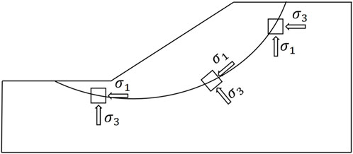
Figure 1. Directions of principal stress at different positions of slope.

If the slope is analyzed under undrained conditions, the undrained shear strength is used to characterize the mechanical behavior of soil. The undrained shear strength is strongly dependent on the angle between the direction of major principal stress and the direction of soil deposition. Previous studies have mostly determined the anisotropic undrained shear strength using Equation 1 (Chen et al., 1975; Al-Karni and Al-Shamrani, 2000):

$c_i=c_h+\left(c_v-c_h\right){\cos }^{2}i(1)$

where $c_v$ and $c_h$ are the undrained shear strength in the vertical (initial sedimentary direction) and horizontal directions, respectively; $i$ is the angle between the direction of the major principal stress and the initial sedimentary direction. The variation of undrained shear strength with major principal stress direction is shown in Figure 2.

Figure 2

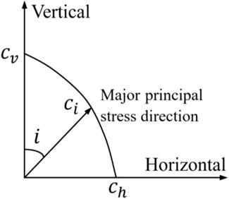
Figure 2. Variation of undrained shear strength with major principal direction.

To indicate the degree of strength anisotropy, a strength anisotropy coefficient is defined by Equation 2:

${k=c_h/c}_v(2)$

The range of the strength anisotropy coefficient is 0∼1.0. The smaller the strength anisotropy coefficient, the stronger the degree of strength anisotropy; Otherwise, the opposite. When the strength anisotropy coefficient is 1.0, the soil is an isotropic material and the undrained shear strength is independent of the direction of principal stress.

After sedimentation, the soil layers undergo rotation under the action of geostress, and the sedimentary direction will rotate (see Figure 3). The angle between the rotated sedimentary direction and the vertical direction (initial sedimentary direction) is called the rotational angle $\beta$. The range of $\beta$ is 0∼ $\pi$. The angle between the direction of the major principal stress and the initial sedimentary direction is denoted as $\alpha$. The angle between the direction of the major principal stress and the rotated sedimentary direction is denoted as $i$.

Figure 3

Figure 3. Initial and rotated soil layers and related angles.

2.2 Slope stability analysis considering strength anisotropy based on ABAQUS

The Mohr Coulomb ideal elastic-plastic model is used to describe the stress-strain relationship of soil and ABAQUS software is used to analyze the slope stability in this paper. There is no Mohr Coulomb model with strength anisotropy in ABAQUS. Therefore, the user-defined material (UMAT) development of Mohr Coulomb model with strength anisotropy must be conducted. This paper adopts an explicit integration algorithm with automatic substepping and error control when developing the UMAT subroutine (Sloan, 1987; Sloan et al., 2001; Zhang and Zhou, 2016; Zhang et al., 2019). It should be noted that in each incremental step, we need to determine the direction of the major principal stress based on the stress state of the element integration point, and then update the undrained shear strength of the soil according to Equation 1. Note that if the soil layers undergo rotation, the angle $i$ in Equation 1 should be the direction of the major principal stress and the rotated sedimentary direction. Then, the updated undrained shear strength is applied to the elastic-plastic calculation of the integration point.

The finite element strength reduction method is a commonly used calculation method of slope safety factor. The basic idea is to reduce the undrained shear strength of the soil until the reduction factor $F$ satisfying a certain instability criterion is found, and then use the reduction factor $F$ at this time as the safety factor ($FS$). In this paper, an algorithm is developed to calculate the safety factors of slopes based on the finite element strength reduction method. The main control program determines the range of $FS$ through dichotomy. The specific steps are as follows:

(1) Give the initial range of the reduction coefficient (for example, 0.1∼10.0). Mark the upper and lower limits of the reduction coefficient as ${FS}_u$ and ${FS}_l$, respectively.

(2) Take the midpoint value (denoted as ${FS}_m$) of the upper and lower limits of the reduction coefficient as the reduction coefficient for this calculation.

(3) Determine the value of undrained shear strength in the rotated sedimentary direction $c_v^{\prime }$ for the calculation based on the reduction coefficient ${FS}_m$ using the formula $c_v^{\prime }=\frac{c_v}{{FS}_m}$. Call the developed UMAT subroutine of Mohr Coulomb model with strength anisotropy for slope stability calculation.

(4) Determine whether the slope stability calculation converges. If the calculation converges, the lower limit of the reduction coefficient is set to be ${FS}_m$, and the upper limit is set to be ${FS}_u$. Otherwise, the lower limit of the reduction coefficient is set to be ${FS}_l$, and the upper limit is set to be ${FS}_m$.

(5) Repeat Steps 2∼4, until the difference between the upper and lower limits of the reduction coefficient is less than the specified error (for example, 0.001). At this time, the midpoint value of the upper and lower limits of the reduction coefficient is taken as the $FS$ of slope.

2.3 Simulation of heterogeneous rotated anisotropy

The heterogeneous rotated anisotropy widely exists in nature (shown in Figure 4), and can be simulated using the random field theory. In the heterogeneous rotated anisotropic soil layers, the scales of fluctuation (SOFs) of undrained shear strength in the strongest and weakest directions of correlation are denoted as ${\theta }_1$ and ${\theta }_2$, respectively. The weakest direction of correlation is the rotated sedimentary direction, and the strongest direction of correlation is perpendicular to the weakest direction of correlation. Generally speaking, ${\theta }_1$ is often greater than ${\theta }_2$. To describe the degree of anisotropy in the spatial distribution of soil parameters, a heterogeneous anisotropy coefficient is defined by Equation 3:

$\lambda =\frac{{\theta }_1}{{\theta }_2}(3)$

Figure 4

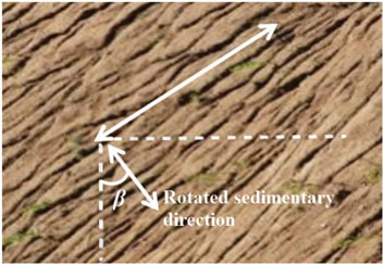
Figure 4. Heterogeneous rotated anisotropy of soil layers.

The larger the heterogeneous anisotropy coefficient, the higher the degree of anisotropy in the soil parameter random field; Otherwise, the opposite. When ${\theta }_1={\theta }_2\left(\lambda =1.0\right)$, the soil parameter random field is isotropic.

In random field theory, autocorrelation functions are often used to describe the autocorrelation between soil parameters at two different spatial positions. There are various types of autocorrelation functions, such as triangular, exponential, Gaussian, and so on. Among them, exponential and Gaussian autocorrelation functions are often used in geotechnical engineering and the exponential autocorrelation function is used in this paper. The formula of exponential autocorrelation function is as follows, see Equation 4:

$\rho \left({\tau }_x,{\tau }_y\right)=\exp \left[-2\sqrt{{\left(\frac{{\tau }_x\cos \beta +{\tau }_y\sin \beta }{{\theta }_1}\right)}^2+{\left(\frac{{\tau }_y\cos \beta -{\tau }_x\sin \beta }{{\theta }_2}\right)}^2}\right](4)$

where ${\tau }_x$ and ${\tau }_y$ are the horizontal and vertical distances between two points, respectively. $\beta$ is the rotational angle.

After determining the autocorrelation function, the domain Ω is divided into $n$ elements, and the centroid coordinates of the elements are denoted as ($x_i$, $y_i$) ($i=1,2,3,\cdots ,n$). Then, the autocorrelation matrix $C$ with $n$ random field elements can be expressed by Equation 5:

$\mathit{C}=\left[\begin{array}{cccc}1& \rho \left({\tau }_{x_{12}},{\tau }_{y_{12}}\right)& \cdots & \rho \left({\tau }_{x_{1n}},{\tau }_{y_{1n}}\right)\\ \rho \left({\tau }_{x_{21}},{\tau }_{y_{21}}\right)& 1& \cdots & \rho \left({\tau }_{x_{2n}},{\tau }_{y_{2n}}\right)\\ ⋮& ⋮& \ddots & ⋮\\ \rho \left({\tau }_{x_{n1}},{\tau }_{y_{n1}}\right)& \rho \left({\tau }_{x_{n2}},{\tau }_{y_{n2}}\right)& \cdots & 1\end{array}\right](5)$

where $\rho \left({\tau }_{x_{ij}},{\tau }_{y_{ij}}\right)$ is the autocorrelation coefficient of soil parameters between element $i$ and element $j$. $\left.{\tau }_{x_{ij}}\left.=\right|x_i-x_j\right|$ and $\left.{\tau }_{y_{ij}}\left.=\right|y_i-y_j\right|$ are the relative distances between element $i$ and element $j$ in the horizontal and vertical directions, respectively. Then, the autocorrelation matrix $\mathit{C}$ can be decomposed into the product of a lower triangular matrix $\mathrm{L}$ and its transpose using the Cholesky decomposition technique (Myers, 1989; Jiang and Huang, 2016), see Equation 6:

$\mathit{C}=\mathit{L}{\mathit{L}}^{\mathrm{T}}(6)$

Suppose $\mathit{\xi }$ is a column vector composed of $n$ independent random variables that follow the standard Gaussian distribution. A Gaussian random field $H_i^D$ can be calculated by Equation 7:

$H_i^D={\displaystyle \sum _{j=1}^n}{L}_{ij}{\xi }_j,i=1,2,3,\cdots ,n(7)$

If the soil parameter $c$ obeys lognormal distribution, the random field of $c$ can be expressed as Equation 8:

$H_i=\exp \left({\mu }_{\ln c}+{\sigma }_{\ln c}{H}_i^D\right),i=1,2,3,\cdots ,n(8)$

where ${\mu }_{\ln c}$ and ${\sigma }_{\ln c}$ are the mean and standard deviation of Gaussian random field $\ln c$, respectively.

2.4 Probabilistic analysis framework of slope stability considering strength anisotropy and heterogeneous rotated anisotropy

To consider strength anisotropy and heterogeneous rotated anisotropy in slope stability analysis, a probabilistic analysis framework is proposed. The probabilistic analysis framework is based on ABAQUS and Python. The flow chart in Figure 5 shows the main steps of the program development of the probabilistic analysis framework. The main steps are as follows:

(1) Collect basis information required for probabilistic slope stability analysis. The information includes the geometric dimensions of slope, the statistical data of heterogeneous rotated anisotropy of soil parameters (distribution type, mean value, coefficient of variation, scales of fluctuation, rotational angle, etc.), and strength anisotropy parameters of soil.

(2) Generate $N$ random fields of heterogeneous rotated anisotropy of soil properties (denoted as $S_1,S_2,\cdots ,S_N$) using the simulation method introduced in Section 2.3 based on the information collected in Step 1.

(3) Establish an initial finite element method (FEM) model of slope with deterministic soil parameters.

(4) The slope safety factor calculation method considering strength anisotropy introduced in Section 2.2 is programmed based on ABAQUS and Python. The developed program is denoted as Code A.

(5) Based on the initial FEM model of the slope, map the generated heterogeneous rotated anisotropy random field $S_i$ into the slope FEM model through Python scripts. Calculate the slope safety factor using Code A and save the safety factor into FS.txt.

(6) Use Python scripts to repeat Step 5, until $N$ slope samples with different random fields are calculated and $N$ safety factors are saved into FS.txt.

(7) Read the data from FS.txt and perform further statistical analysis.

Figure 5

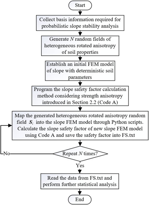
Figure 5. Flow chart of the proposed probabilistic analysis framework.

3 Case study

Taking a cohesive soil slope as an example, the influence of strength anisotropy and heterogeneous rotated anisotropy on slope stability is investigated in this section. As shown in Figure 6, the height of the slope is 5m, and the slope angle is 45°. Assuming undrained conditions, the undrained shear strength in the rotated sedimentary direction $C_v$ follows the Log-normal distribution. The mean value of $C_v$ is 40 kPa, the coefficient of variation of $C_v$ is 0.2, and the scale of fluctuation in the rotated sedimentary direction (${\theta }_2$) is 1.0 m. Other soil parameters are assumed to be determined values. The weight of soil $\gamma$ is 20 $\text{kN}/{\mathrm{m}}^3$, the elastic modulus $E$ is 100$\text{MPa}$, and the Poisson's ratio $\nu$ is 0.3.

Figure 6

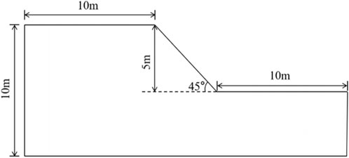
Figure 6. Slope geometry model.

3.1 Deterministic analysis

The deterministic analysis is conducted first using the developed finite element algorithm introduced in Section 2.4. All soil parameters are considered as determined values. Take 40 kPa as the value of $C_v$ which is the undrained shear strength in the rotated sedimentary direction to conduct the deterministic analysis. Four schemes named Schemes A1∼A4 are adopted, in which the strength anisotropy coefficients are 0.4, 0.6, 0.8, and 1.0, respectively. Figure 7 shows the $FS$ variation with the rotational angles under different strength anisotropy coefficients. It can be seen that the strength anisotropy coefficient has a significant influence on slope stability. When the strength anisotropy coefficient is 1.0 (Scheme A4), the $FS$ of the slope is 2.16, and it does not vary with rotational angles. There is little difference between this calculated result and the result 2.18 obtained by Cheng et al. (2017) using FLAC software, which confirmed the validity of the developed algorithm. When the strength anisotropy coefficient is little than 1.0, the variation law of $FS$ with rotational angles is almost the same. As the rotational angle increases, the $FS$ first increases, then decreases, and then increases again. The greatest value of $FS$ appears at 30$°$, and the slope is a reverse slope at this time. The smallest value of $FS$ appears between 105$°$ and 120$°$. The slope is a dip slope at this time. This change pattern is consistent with the usual pattern of “dip slopes are prone to failure, while reverse slopes are less prone to failure.” The rotational angle corresponding to the minimum safety factor decreases as the strength anisotropy coefficient decreases. In addition, the smaller the strength anisotropy coefficient, the smaller the undrained shear strength perpendicular to the rotated sedimentary direction, and the lower the stability of the slope under the same rotational angle.

Figure 7

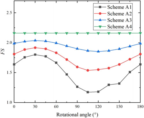
Figure 7. Variation of FS with rotational angles under different strength anisotropy coefficients.

3.2 Stochastic analysis

3.2.1 Simulation of rotational anisotropy random field of soil parameters

To consider the impact of rotational anisotropy of soil parameters on slope stability, the rotational anisotropy random field of soil parameters should be generated first. The steps for generating rotational anisotropy random field of soil parameters are introduced in Section 2.3. Figure 8 shows the random field of undrained shear strength $c_v$ when the heterogeneous anisotropy coefficient $\lambda$ is 10.0, and the rotational angle $\beta$ is 120$°$. It can be seen that the generated random field effectively simulates the characteristics of spatial variation of soil parameters and the rotation of strata. When the strength anisotropy coefficient $k$ is 0.6, the undrained shear strength $c_h$ is 0.6 times as much as $c_v$ for the same element.

Figure 8

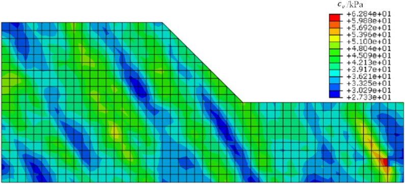
Figure 8. Random field of undrained shear strength $c_v$.

3.2.2 Determination of the number of simulations

To obtain accurate statistics of $FS$ and reduce the calculation amount, it is necessary to determine an appropriate number of simulations. The number of simulations is taken as 2000, the strength anisotropy coefficient $k$ is taken as 0.6, the heterogeneous anisotropy coefficient $\lambda$ is taken as 10.0, and the rotational angle $\beta$ is taken as 120$°$. Then, use the proposed algorithm introduced in Section 2.4 to conduct the stochastic analysis. The results are shown in Figure 9. It can be seen that when the number of simulations is greater than 1000, the mean value and the coefficient of variation of $FS$ are stable. Therefore, 1000 is taken as the number of simulations in this paper.

Figure 9

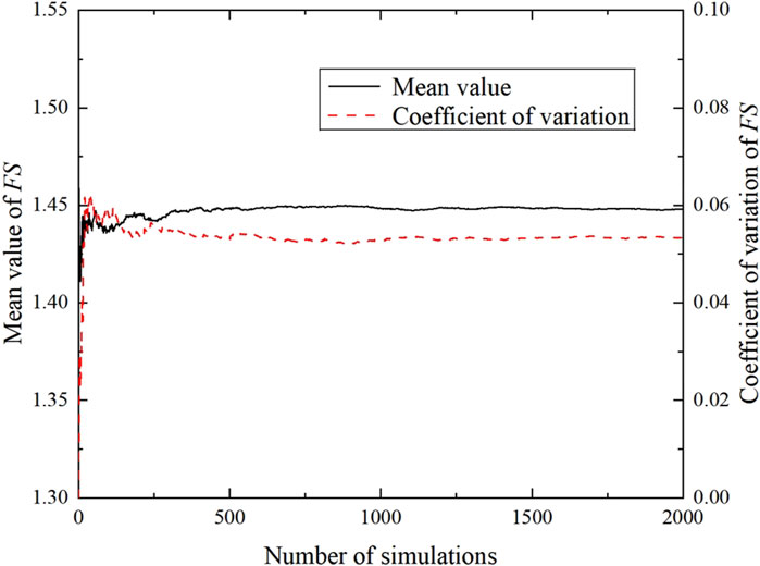
Figure 9. Variations of statistics of $FS$ with the number of simulations.

3.2.3 Influence of strength anisotropy and heterogeneous rotated anisotropy on slope stability

To study the influence of strength anisotropy and heterogeneous rotated anisotropy on slope reliability, 16 calculation schemes (shown in Table 1) with different strength coefficients, heterogeneous anisotropy coefficients, and rotational angles, are adopted to conduct the slope stability analysis.

Table 1

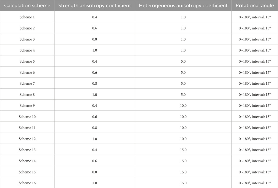
Table 1. Parameters of various calculation schemes.

Assuming $FS$ obey the normal distribution. Therefore, the reliability index denoted as ${\beta }_R$, can be calculated by Equation 9:

${\beta }_R=\frac{{\mu }_{FS}-1}{{\sigma }_{FS}}(9)$

where ${\mu }_{FS}$ and ${\sigma }_{FS}$ are the mean value and standard deviation of $FS$, respectively. The variation of statistics of $FS$ with rotational angles under the same heterogeneous anisotropy coefficient and different strength anisotropy coefficient conditions is shown in Figures 10–13. It can be seen that the statistics of $FS$ including mean value, coefficient of variation, and reliability index, vary with rotational angles except for Scheme 4. When the strength anisotropy coefficient is 1.0, and the heterogeneous anisotropy is 1.0 (Scheme 4), the mean value, the coefficient of variation of $FS$, and the reliability index do not change with the increase of the rotational angle. In Scheme 4, the mean value and the coefficient of variation of $FS$ are 2.06 and 0.025, which is generally consistent with the results calculated by Cheng et al. (2017) using FLAC software. For other schemes, the mean value of $\text{FS}$ increases first, then decreases, and then increases with the increase of the rotational angle. The relationship curve between the mean value of $FS$ and the rotational angle is influenced by the strength anisotropy coefficient. When the strength anisotropy coefficient is greater, the mean value of $FS$ varies weaker as the rotational angle increases. The relationship curve between the mean value of $FS$ and the rotational angle with a greater strength anisotropy coefficient is always above that with a smaller strength anisotropy coefficient. It means that if the strength anisotropy coefficient is ignored (i.e., the strength anisotropy coefficient is taken as 1.0), the mean value of $FS$ will be overestimated. The mean value of $FS$ versus rotational angle curves of the 16 schemes are the compared with that of Schemes A1∼A4. Note that in Schemes A1∼A4, only the strength anisotropy is considered in the slope stability analysis, and the heterogeneous rotated anisotropy is not considered. It can be seen that when the heterogeneous rotated anisotropy is considered, the change law of the mean value of $FS$ with the rotational angle is the same as that when only the strength anisotropy is considered. But the mean value of $FS$ is smaller than that only the strength anisotropy is considered. This is because when calculating the $FS$ of the slope, the program will automatically search for the route with the weakest undrained shear strength and form the corresponding sliding surface. The influence of elements with lower undrained shear strength on the slope stability calculation is more important than that of elements with higher undrained shear strength.

Figure 10

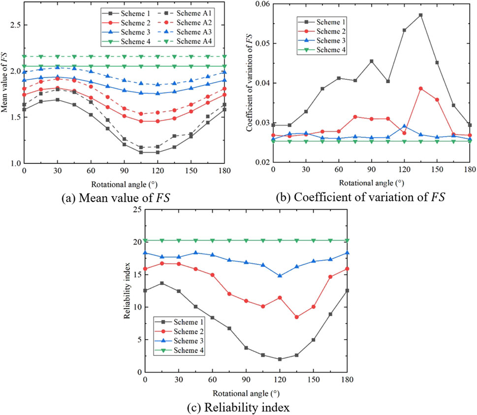
Figure 10. Variation of statistics of $FS$ with rotational angles (λ = 1.0). (a) Mean value of $FS$. (b) Coefficient of variation of $FS$. (c) Reliability index.

Figure 11

Figure 11. Variation of statistics of $FS$ with rotational angles (λ = 5.0). (a) Mean value of $FS$. (b) Coefficient of variation of $FS$. (c) Reliability index.

Figure 12

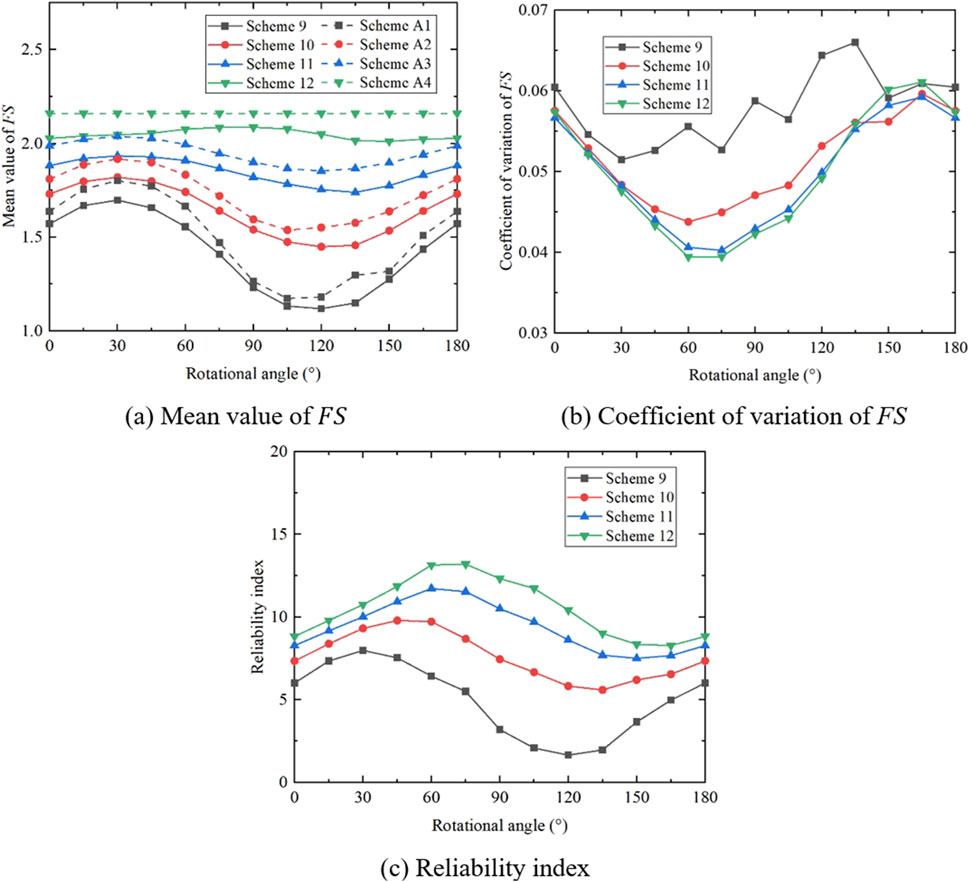
Figure 12. Variation of statistics of $FS$ with rotational angles (λ = 10.0). (a) Mean value of $FS$. (b) Coefficient of variation of FS. (c) Reliability index.

Figure 13

Figure 13. Variation of statistics of $FS$ with rotational angles (λ = 15.0). (a) Mean value of $FS$. (b) Coefficient of variation of $FS$. (c) Reliability index.

The coefficient of variation of $FS$ is also influenced by the rotational angle except for Scheme 4. The change law of the coefficient of variation of $FS$ with the rotational angle is relatively complicated. In Schemes 1∼3, the heterogeneous anisotropy coefficient is 1.0, and the variation of the coefficient of variation of $FS$ with the rotational angle is all due to the strength anisotropy. There are multiple extremes on the curve of the coefficient of variation of $FS$ versus the rotational angle in Schemes 1∼3. With different strength coefficients, the rotational angles corresponding to the extreme points are different. For other schemes, the change law of the coefficient of variation of $FS$ with the rotational angle is almost the same. When the strength anisotropy coefficient is greater than 0.4, with the increase of the rotational angle, the coefficient of variation of $FS$ decreases first, then increases, and then decreases again. The minimum and the maximum values of the coefficient of variation of $FS$ are related to the strength anisotropy coefficient and the heterogeneous anisotropy coefficient. Whereas the rotational angles corresponding to the minimum and maximum values are relatively fixed and less affected by these two coefficients, which are located at about $60°$ ∼$75°$ and $165°$, respectively. When the strength anisotropy coefficient is 0.4, the strength anisotropy of soil is strong and the influence on the relationship curve between the coefficient of variation of $FS$ and the rotational angle is also stronger. At this time, the change law of the coefficient of variation of $FS$ with the rotational angle is more complicated. The strength anisotropy coefficient also has an important influence on the value of the coefficient of variation of $FS$. When the strength anisotropy coefficient is smaller, the coefficient of variation of $FS$ is greater under the same rotational angle, and the coefficient of variation of $FS$ varies more strongly with the rotational angle. The curve of the coefficient of variation of $FS$ versus the rotational angle with smaller strength anisotropy coefficient is usually above that with greater strength anisotropy coefficient.

As for the reliability index, the change law of the reliability index with the rotational angle is similar to that of the mean value of $FS$ with the rotational angle. For the schemes except for Schemes 3 and 4, the reliability index increases first, then decreases, and then increases again. The positions of the minimum and maximum values are influenced by the strength anisotropy coefficient. As the strength anisotropy increases, the positions of the minimum and maximum values will move to the right, i.e., the corresponding rotational angle increases. If the strength anisotropy is not considered, the reliability index of the slope will be overestimated, and the most unfavorable rotational angle of the strata will be significantly different from the actual situation.

To better study the influence of the heterogeneous anisotropy coefficient on slope stability, the calculation results of the 16 schemes are drawn with the same strength anisotropy coefficient and different heterogeneous anisotropy coefficients (see Figures 14–17). It can be seen that under the same strength anisotropy coefficient, with the increase of the heterogeneous anisotropy coefficient, there is little difference in the curves of the mean value of $FS$ versus the rotational angle, whereas there is a significant difference in the curves of the coefficient of variation of $FS$ versus the rotational angle. Under the same rotational angle, with the increase of the heterogeneous anisotropy coefficient, the coefficient of variation of $FS$ increases, and the relationship curve between the coefficient of variation of $FS$ and the rotational angle will also move up. Under different heterogeneous anisotropy coefficients and the same strength anisotropy coefficient, the change law of the coefficients of variation of $FS$ with the rotational angle is almost the same except for Schemes 1∼4 (heterogeneous anisotropy coefficient is 1.0). The change law is that with the increase of the rotational angle, the coefficient of variation of $FS$ generally decreases first, then increases and then decreases again. When the strength anisotropy is greater than 0.4, the change law is stable and the positions of the minimum and maximum values are almost the same. When the strength anisotropy is 0.4, the overall change law is the same, but some fluctuations exist. The relationship curves between the reliability index and the rotational angle with different heterogeneous anisotropy coefficients and the same strength anisotropy coefficient have obvious differences, which indicates that the heterogeneous anisotropy coefficient has an important influence on the reliability index of the slope. With the increase of the heterogeneous anisotropy coefficient, the relationship curves between the reliability index and the rotational angle move down. The rotational angles corresponding to the minimum and maximum values of the reliability index are little influenced by the heterogeneous anisotropy coefficient under the same strength anisotropy coefficient (except for Schemes 1∼4).

Figure 14

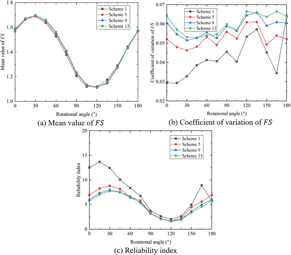
Figure 14. Variation of statistics of $FS$ with rotational angles (k = 0.4). (a) Mean value of $FS$. (b) Coefficient of variation of $FS$. (c) Reliability index.

Figure 15

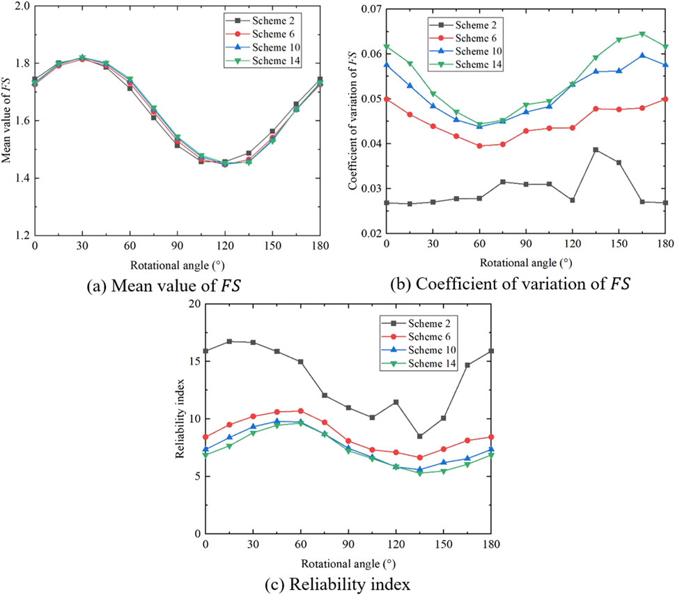
Figure 15. Variation of statistics of $FS$ with rotational angles (k = 0.6). (a) Mean value of $FS$. (b) Coefficient of variation of $FS$. (c) Reliability index.

Figure 16

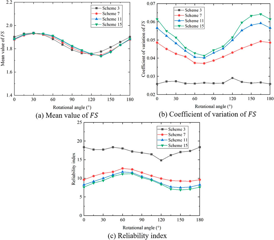
Figure 16. Variation of statistics of $FS$ with rotational angles (k = 0.8). (a) Mean value of $FS$. (b) Coefficient of variation of $FS$. (c) Reliability index.

Figure 17

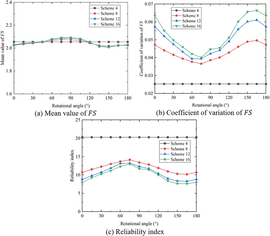
Figure 17. Variation of statistics of $FS$ with rotational angles (k = 1.0). (a) Mean value of $FS$. (b) Coefficient of variation of $FS$. (c) Reliability index.

4 Conclusion

In this paper, a probabilistic analysis framework of slope stability considering the coupled effect of strength anisotropy and heterogeneous rotated anisotropy is proposed. The slope stability under different degrees of strength anisotropy and heterogeneous rotated anisotropy is analyzed. The main conclusions can be drawn as follows:

(1) The proposed probabilistic analysis framework of slope stability considering the coupled effect of strength anisotropy and heterogeneous rotated anisotropy is effective.

(2) Under the same rotational angle, the $FS$ calculated when considering the strength anisotropy is smaller than that when neglecting the strength anisotropy, and the mean value of $FS$ calculated when considering the spatial variability of soil parameters is smaller than the $FS$ of the corresponding homogeneous soil slope. If the strength anisotropy or the heterogeneous rotated anisotropy is not considered, the stability of the slope will be overestimated.

(3) The strength anisotropy coefficient, the heterogeneous anisotropy coefficient, and the rotational angle have important effects on slope stability. The mean value of $FS$ varies greatly with the strength anisotropy coefficient and the rotational angle, and is not sensitive to the heterogeneous anisotropy coefficient. Generally speaking, the smaller the strength anisotropy coefficient and the larger the heterogeneous anisotropy coefficient are, then the smaller the mean value of $FS$ is, the larger the coefficient of variation of $FS$ is, and the smaller the reliability index is.

(4) The rotational angles corresponding to the minimum and maximum values of the reliability index are greatly influenced by the strength anisotropy coefficient but are less affected by the heterogeneous anisotropy coefficient. With the increase of the strength anisotropy coefficient, the safest rotational angles can increase from 30$°$ to 75$°$, and the most dangerous rotational angles can increase from 120$°$ to 165$°$. However, with the increase of the heterogeneous anisotropy coefficient, the safest and most dangerous rotational angles are almost the same.

Data availability statement

The original contributions presented in the study are included in the article/supplementary material, further inquiries can be directed to the corresponding author.

Author contributions

WC: Conceptualization, Methodology, Software, Validation, Writing – original draft, Writing – review and editing. WL: Methodology, Validation, Visualization, Writing – review and editing. HY: Data curation, Software, Writing – review and editing. YL: Funding acquisition, Software, Visualization, Writing – review and editing.

Funding

The author(s) declare that financial support was received for the research and/or publication of this article. This research was funded by the National Natural Science Foundation of China (Project Nos 42177170 and 52004090), the Natural Science Foundation of Hebei Province (Project Nos E2021508031 and E2024508032) and the Fundamental Research Funds for the Central Universities (3142021010). The financial support is greatly acknowledged.

Conflict of interest

The authors declare that the research was conducted in the absence of any commercial or financial relationships that could be construed as a potential conflict of interest.

Generative AI statement

The author(s) declare that no Gen AI was used in the creation of this manuscript.

Publisher’s note

All claims expressed in this article are solely those of the authors and do not necessarily represent those of their affiliated organizations, or those of the publisher, the editors and the reviewers. Any product that may be evaluated in this article, or claim that may be made by its manufacturer, is not guaranteed or endorsed by the publisher.

References

Al-Karni, A. A., and Al-Shamrani, M. A. (2000). Study of the effect of soil anisotropy on slope stability using method of slices. Comput. Geotech. 26 (2), 83–103. doi:10.1016/S0266-352X(99)00046-4

CrossRef Full Text | Google Scholar

Azarafza, M., Akgün, H., Ghazifard, A., Asghari-Kaljahi, E., Rahnamarad, J., and Derakhshani, R. (2021). Discontinuous rock slope stability analysis by limit equilibrium approaches–a review. Int. J. Digit. Earth. 14 (12), 1918–1941. doi:10.1080/17538947.2021.1988163

CrossRef Full Text | Google Scholar

Bozorgpour, M. H., Binesh, S. M., and Rahmani, R. (2021). Probabilistic stability analysis of geo-structures in anisotropic clayey soils with spatial variability. Comput. Geotech. 133, 104044. doi:10.1016/j.compgeo.2021.104044

CrossRef Full Text | Google Scholar

Chen, L., Zhang, W., Chen, F., Gu, D., Wang, L., and Wang, Z. (2022). Probabilistic assessment of slope failure considering anisotropic spatial variability of soil properties. Geosci. Front. 13 (3), 101371. doi:10.1016/j.gsf.2022.101371

CrossRef Full Text | Google Scholar

Chen, W. F., Snitbhan, N., and Fang, H. Y. (1975). Stability of slopes in anisotropic, nonhomogeneous soils. Can. Geotech. J. 12 (1), 146–152. doi:10.1139/t75-014

CrossRef Full Text | Google Scholar

Cheng, H. Z., Chen, J., Wang, Z. S., Hu, Z. F., and Huang, J. H. (2017). Stability analysis of a clay slope accounting for the rotated anisotropy correlation structure. Chin. J. Rock Mech. Eng. 36 (S2), 3965–3973. doi:10.13722/j.cnki.jrme.2017.0044

CrossRef Full Text | Google Scholar

Dasaka, S. M., and Zhang, L. M. (2012). Spatial variability of in situ weathered soil. Geotechnique 62 (5), 375–384. doi:10.1680/geot.8.P.151.3786

CrossRef Full Text | Google Scholar

Deng, Z. P., Li, D. Q., Qi, X. H., Cao, Z. J., and Phoon, K. K. (2017). Reliability evaluation of slope considering geological uncertainty and inherent variability of soil parameters. Comput. Geotech. 92, 121–131. doi:10.1016/j.compgeo.2017.07.020

CrossRef Full Text | Google Scholar

Deng, Z. P., Pan, M., Niu, J. T., and Jiang, S. H. (2022). Full probability design of soil slopes considering both stratigraphic uncertainty and spatial variability of soil properties. Bull. Eng. Geol. Environ. 81 (5), 195. doi:10.1007/s10064-022-02702-2

CrossRef Full Text | Google Scholar

Ding, Y. N., Li, D. Q., Zarei, C., Yi, B. L., and Liu, Y. (2021). Probabilistically quantifying the effect of geotechnical anisotropy on landslide susceptibility. Bull. Eng. Geol. Environ. 80, 6615–6627. doi:10.1007/s10064-021-02197-3

CrossRef Full Text | Google Scholar

Elkateb, T., Chalaturnyk, R., and Robertson, P. K. (2003). An overview of soil heterogeneity: quantification and implications on geotechnical field problems. Can. Geotech. J. 40 (1), 1–15. doi:10.1139/t02-090

CrossRef Full Text | Google Scholar

Griffiths, D. V., and Fenton, G. A. (2001). Bearing capacity of spatially random soil: the undrained clay Prandtl problem revisited. Geotechnique 51 (4), 351–359. doi:10.1680/geot.2001.51.4.351

CrossRef Full Text | Google Scholar

Huang, L., Cheng, Y. M., Leung, Y. F., and Li, L. (2019). Influence of rotated anisotropy on slope reliability evaluation using conditional random field. Comput. Geotech. 115, 103133. doi:10.1016/j.compgeo.2019.103133

CrossRef Full Text | Google Scholar

Huang, L., Cheng, Y. M., Li, L., and Yu, S. (2021). Reliability and failure mechanism of a slope with non-stationarity and rotated transverse anisotropy in undrained soil strength. Comput. Geotech. 132, 103970. doi:10.1016/j.compgeo.2020.103970

CrossRef Full Text | Google Scholar

Hwang, J., Dewoolkar, M., and Ko, H. Y. (2002). Stability analysis of two-dimensional excavated slopes considering strength anisotropy. Can. Geotech. J. 39, 1026–1038. doi:10.1139/t02-057

CrossRef Full Text | Google Scholar

Jiang, S. H., and Huang, J. S. (2016). Efficient slope reliability analysis at low-probability levels in spatially variable soils. Comput. Geotech. 75, 18–27. doi:10.1016/j.compgeo.2016.01.016

CrossRef Full Text | Google Scholar

Jiang, S. H., Li, D. Q., Zhang, L. M., and Zhou, C. B. (2014). Slope reliability analysis considering spatially variable shear strength parameters using a non-intrusive stochastic finite element method. Eng. Geol. 168, 120–128. doi:10.1016/j.enggeo.2013.11.006

CrossRef Full Text | Google Scholar

Li, J. Z., Zhang, S. H., Liu, L. L., Huang, L., Cheng, Y. M., and Dias, D. (2022). Probabilistic analysis of pile-reinforced slopes in spatially variable soils with rotated anisotropy. Comput. Geotech. 146, 104744. doi:10.1016/j.compgeo.2022.104744

CrossRef Full Text | Google Scholar

Li, X. Y., Zhang, L. M., and Li, J. H. (2016). Using conditioned random field to characterize the variability of geologic profiles. J. Geotech. Geoenviron. Eng. 142, 04015096. doi:10.1061/(asce)gt.1943-5606.0001428

CrossRef Full Text | Google Scholar

Li, Y., Goh, A. T. C., Zhang, R., and Zhang, W. (2023). Stability charts for undrained clay slopes considering soil anisotropic characteristics. Bull. Eng. Geol. Environ. 82 (2), 52. doi:10.1007/s10064-023-03067-w

CrossRef Full Text | Google Scholar

Liu, L., Liang, C., Xu, M., Zhu, W., Zhang, S., and Ding, X. (2023). Probabilistic analysis of large slope deformation considering soil spatial variability with rotated anisotropy. J. Earth Sci. 48 (5), 1836–1852. doi:10.3799/dqkx.2022.372

CrossRef Full Text | Google Scholar

Ma, G., Rezania, M., Mousavi Nezhad, M., and Hu, X. (2022). Uncertainty quantification of landslide runout motion considering soil interdependent anisotropy and fabric orientation. Landslides 19, 1231–1247. doi:10.1007/s10346-021-01795-2

CrossRef Full Text | Google Scholar

Ma, N., and Yao, Z. (2024). Analysis of slope stochastic fields using a novel deep learning model with attention mechanism. Front. Earth Sci. 12, 1352958. doi:10.3389/feart.2024.1352958

CrossRef Full Text | Google Scholar

Myers, D. E. (1989). Vector conditional simulation. Geostatistics 4, 283–293. doi:10.1007/978-94-015-6844-9_21

CrossRef Full Text | Google Scholar

Nanehkaran, Y. A., Licai, Z., Chengyong, J., Chen, J., Anwar, S., Azarafza, M., et al. (2023). Comparative analysis for slope stability by using machine learning methods. Appl. Sci. 13 (3), 1555. doi:10.3390/app13031555

CrossRef Full Text | Google Scholar

Nanehkaran, Y. A., Pusatli, T., Chengyong, J., Chen, J., Cemiloglu, A., Azarafza, M., et al. (2022). Application of machine learning techniques for the estimation of the safety factor in slope stability analysis. Water 14 (22), 3743. doi:10.3390/w14223743

CrossRef Full Text | Google Scholar

Ng, C. W. W., Qu, C., Ni, J., and Guo, H. (2022). Three-dimensional reliability analysis of unsaturated soil slope considering permeability rotated anisotropy random fields. Comput. Geotech. 151, 104944. doi:10.1016/j.compgeo.2022.104944

CrossRef Full Text | Google Scholar

Nian, T. K., Chen, G. Q., Luan, M. T., Yang, Q., and Zheng, D. F. (2008). Limit analysis of the stability of slopes reinforced with piles against landslide in nonhomogeneous and anisotropic soils. Can. Geotech. J. 45, 1092–1103. doi:10.1139/T08-042

CrossRef Full Text | Google Scholar

Phoon, K. K., and Kulhawy, F. H. (1999). Characterization of geotechnical variability. Can. Geotech. J. 36 (4), 612–624. doi:10.1139/t99-038

CrossRef Full Text | Google Scholar

Shogaki, T., and Kumagai, N. (2008). A slope stability analysis considering undrained strength anisotropy of natural clay deposits. Soils Found. 48, 805–819. doi:10.3208/sandf.48.805

CrossRef Full Text | Google Scholar

Sloan, S. W. (1987). Substepping schemes for the numerical integration of elastoplastic stress–strain relations. Int. J. Numer. Anal. Methods Geomech. 24, 893–911. doi:10.1002/nme.1620240505

CrossRef Full Text | Google Scholar

Sloan, S. W., Abbo, A. J., and Sheng, D. (2001). Refined explicit integration of elastoplastic models with automatic error control. Eng. Comput. 18, 121–194. doi:10.1108/02644400110365842

CrossRef Full Text | Google Scholar

Tang, H. X., and Wei, W. C. (2019). Finite element analysis of slope stability by coupling of strength anisotropy and strain softening of soil. Rock Soil Mech. 40 (10), 4092–4100. doi:10.16285/j.rsm.2019.0164

CrossRef Full Text | Google Scholar

Tang, H. X., Wei, W. C., Liu, F., and Chen, G. Q. (2020). Elastoplastic cosserat continuum model considering strength anisotropy and its application to the analysis of slope stability. Comput. Geotech. 117, 103235. doi:10.1016/j.compgeo.2019.103235

CrossRef Full Text | Google Scholar

Tian, X., Song, Z., Wang, H., Cheng, Y., and Wang, J. (2024a). Deformation and mechanical characteristics of tunnel-slope systems with existing anti-slide piles under the replacement structure of pile-wall. Tunn. Undergr. Sp. Tech. 153, 105995. doi:10.1016/j.tust.2024.105995

CrossRef Full Text | Google Scholar

Tian, X., Song, Z., Wang, T., Xie, J., Cheng, Y., and Liu, Z. (2024b). Theoretical analysis of additional surrounding rock pressure in shallow buried bias tunnel. Sci. Rep. 14 (1), 30788. doi:10.1038/s41598-024-80658-x

CrossRef Full Text | Google Scholar

Wang, D., and Jin, X. (2008). Slope stability analysis by finite elements considering strength anisotropy. Rock Soil Mech. 29 (3), 667–672. doi:10.3969/j.issn.1000-7598.2008.03.018

CrossRef Full Text | Google Scholar

Wang, Z., Wang, H., and Xu, W. (2021). Effect of rotated anisotropy of soil shear strength on three-dimensional slope stability: a probabilistic analysis. Bull. Eng. Geol. Environ. 80 (8), 6527–6538. doi:10.1007/s10064-021-02336-w

CrossRef Full Text | Google Scholar

Xia, C., Lu, G., Zhu, Z., Wu, L., Zhang, L., Luo, S., et al. (2020). Deformation and stability characteristics of layered rock slope affected by rainfall based on anisotropy of strength and hydraulic conductivity. Water 12 (11), 3056. doi:10.3390/w12113056

CrossRef Full Text | Google Scholar

Yu, H. S., and Sloan, S. W. (1994). Limit analysis of anisotropic soils using finite elements and linear programming. Mech. Res. Commun. 21 (6), 545–554. doi:10.1016/0093-6413(94)90017-5

CrossRef Full Text | Google Scholar

Zhang, Y., and Zhou, A. (2016). Explicit integration of a porosity-dependent hydro-mechanical model for unsaturated soils. Int. J. Numer. Anal. Methods Geomech. 40 (17), 2353–2382. doi:10.1002/nag.2533

CrossRef Full Text | Google Scholar

Zhang, Y., Zhou, A., Nazem, M., and Carter, J. (2019). Finite element implementation of a fully coupled hydro-mechanical model and unsaturated soil analysis under hydraulic and mechanical loads. Comput. Geotech. 110, 222–241. doi:10.1016/j.compgeo.2019.02.005

CrossRef Full Text | Google Scholar

Zhu, H., and Zhang, L. M. (2013). Characterizing geotechnical anisotropic spatial variations using random field theory. Can. Geotech. J. 50 (7), 723–734. doi:10.1139/cgj-2012-0345

CrossRef Full Text | Google Scholar

Zhu, H., Zhang, L. M., and Xiao, T. (2019). Evaluating stability of anisotropically deposited soil slopes. Can. Geotech. J. 56 (5), 753–760. doi:10.1139/cgj-2018-0210

CrossRef Full Text | Google Scholar