On a planetary forcing of global seismicity

Dumont, Stéphanie; de Bremond d’Ars, Jean; Boulé, Jean-Baptiste; Courtillot, Vincent; Gèze, Marc; Gibert, Dominique; Kossobokov, Vladimir; Le Mouël, Jean-Louis; Lopes, Fernando; Neves, Maria C.; Silveira, Graça; Petrosino, Simona; Zuddas, Pierpaolo

doi:10.3389/feart.2025.1587650

ORIGINAL RESEARCH article

Front. Earth Sci., 02 July 2025

Sec. Solid Earth Geophysics

Volume 13 - 2025 | https://doi.org/10.3389/feart.2025.1587650

This article is part of the Research TopicWhen The Earth Records CyclesView all articles

On a planetary forcing of global seismicity

Stéphanie Dumont¹*

Jean de Bremond d’Ars²

Marc Gèze⁵^†

Jean-Louis Le Mouël⁴

Graça Silveira^1,9

Simona Petrosino¹⁰

Pierpaolo Zuddas¹¹

¹IDL - Instituto Dom Luiz, Faculdade de Ciências, Universidade de Lisboa, Lisboa, Portugal
²University Rennes, CNRS, Géosciences Rennes, UMR 6118, Rennes, France
³Muséum National d’Histoire Naturelle, CNRS UMR 7196, INSERM U1154, Sorbonne Université, Paris, France
⁴Académie des Sciences de Paris, Paris, France
⁵Muséum National d’Histoire Naturelle, CEMIM, Sorbonne Université, Paris, France
⁶LGL-TPE, University Lyon, University Lyon 1, ENSL, CNRS, UMR, Villeurbanne, France
⁷Institute of Earthquake Prediction Theory and Mathematical Geophysics, Russian Academy of Sciences, Moscow, Russia
⁸FCT, Campus de Gambelas, Universidade do Algarve, Faro, Portugal
⁹Instituto Superior de Engenharia de Lisboa (ISEL), Instituto Politécnico de Lisboa, Lisboa, Portugal
¹⁰Istituto Nazionale di Geofisica e Vulcanologia, Sezione di Napoli—Osservatorio Vesuviano, Naples, Italy
¹¹Sorbonne Université, CNRS, METIS, Paris, France

We have explored the temporal variability of the seismicity at global scale over the last 124 years, as well as its potential drivers. To achieve this, we constructed and analyzed an averaged global seismicity curve for earthquakes of magnitude equal or greater than 6.0 since 1900. Using Singular Spectrum Analysis, we decomposed this curve and compared the extracted pseudo-cycles with two global geophysical parameters associated with Earth’s tides: length-of-day variations and sea-level changes. Our results reveal that these three geophysical signal curves can be reconstructed up to ∼90% by the sum of up to seven periodic components ranging from 1 to ∼60 years, largely aligned with planetary ephemerides. We discuss these results in the framework of Laplace’s theory, with a particular focus on the phase relationships between seismicity, length-of-day variations, and sea-level changes to further elucidate the underlying physical mechanisms. Finally, integrating observations from seismogenic regions, we propose a possible trigger mechanism based on solid Earth–hydrosphere interactions, emphasizing the key role of water-rock interactions in modulating earthquake occurrence.

1 Introduction

The question of apparent random nature of earthquakes remains an important and contemporary topic (e.g., Gardner and Knopoff, 1974; Heaton, 1975; Klein, 1976; Kilston and Knopoff, 1983; Mazzarella and Palumbo, 1989; Lopes et al., 1990; Kossobokov, 2006; Métivier et al., 2009; De Santis et al., 2010; Hough, 2018; Varga and Grafarend, 2019; Kossobokov and Panza, 2020). An earthquake is a sudden movement within the Earth’s lithosphere. Earthquake occurrences are not random, but rather haphazard, i.e., lacking any obvious principle of organization, obeying the Unified Earthquake Scaling Law (Kossobokov, 2021), which generalizes the fundamental Gutenberg-Richter relation (Gutenberg and Richter, 1954). Mathematically, the characteristics of such haphazard systems, apparently chaotic, are nevertheless predictable up to a certain limit and after substantial averaging. In particular, the results of on-going global testing of the earthquake prediction algorithm M8 started in 1992 (Healy et al., 1992; Ismail-Zadeh and Kossobokov, 2021) have provided evidence of predictability for most of the world largest earthquakes, although up to a certain space-time limit of intermediate-term middle-range accuracy This mathematical framework is one of several approaches used to explore seismogenic processes—highly non-linear phenomena rooted in the Earth’s dynamic behavior, to improve our predictive capabilities. Seismic activity resulting from tectonic stress and deformation between lithospheric plates involve intricate, multi-scale processes that extend from deep within the mantle to near-surface levels with impact on Earth’s rotation parameters (e.g., Jault and Le Mouël, 1991; Le Mouël et al., 2023). These mechanisms operate and interact across a broad spectrum of temporal and spatial scales, contributing to the variability and distribution of seismic activity both regionally and globally (Turcotte and Malamud, 2002; Khain and Goncharov, 2006; Sobolev, 2011; Yoshida and Santosh, 2011; Muldashev and Sobolev, 2020; Zaccagnino et al., 2020; Zaccagnino and Doglioni, 2022).

For seismic events, the notion of “preferred days” or “astronomical forcing” is an ancient concept first found in the writings of Pliny the Elder (77), with a renewed interest due to Perrey (1875), who regarded lunar forces as the primary driver. Regardless of the presumed nature of this forcing, studies have long tended not merely to minimize but to invalidate the concept of external forcing, such as tidal effects, by mainly relying on fracture and stress/strain mechanics principles (e.g., Rydelek et al., 1992; Vere-Jones, 1995; Jordan et al., 2011), and therefore on physical considerations, with seldom reference to (geo)chemical processes (e.g., Teng, 1980; Toutain and Baubron, 1999; Perez et al., 2008; Woith, 2015).

The Lisbon earthquake of 1755, undoubtedly the first earthquake to be documented with the rigor and standards of a contemporary scientific article, shows a remarkable singularity in the robustness of its observations (e.g., Pereira de Sousa, 1919; Baptista et al., 1998; Poirier, 2005; Poirier, 2006). Unfortunately, not all seismic events around the world have been documented with the same quality. Most studies dealing with global seismicity start at the beginning of the 20th century and focus not on historical but rather on instrumental records even when they critically examine the available seismic catalogues (e.g., Healy et al., 1992; Engdahl and Villaseñor, 2002; Kagan, 2003; Albini et al., 2014; Kossobokov and Panza, 2020). Independent studies focused on regional and global seismicity and conducted over time have used spectral analyses to investigate the temporal distribution of strong, significant or even great earthquakes (e.g., Liritzis and Tsapanos, 1993; Malyshkov and Malyshkov, 2009; Scafetta and Mazzarella, 2015). These studies have identified periodicities around ∼5 years, ∼7 years, ∼8 years, ∼11 years, ∼14 years, ∼18 years, ∼20 years, and ∼40 years. Of course, it is important to bear in mind that spectral analysis is known to be challenging for strictly non-stationary signals (e.g., Kay and Marple, 1981; Gibert et al., 2024, chapter 11). Comparing these results is further complicated by variations in the datasets used, which often differ in spatial scale (regional vs global) and magnitude thresholds, making direct comparisons challenging. Nevertheless, these periodicities are to some extent consistent with Laplace commensurabilities, i.e., orbital resonances of celestial bodies (cf. Mörth and Schlamminger, 1979; Lopes et al., 2021). These periods, which are more or less compatible over a common timescale with those observed for average global volcanism (cf. Dumont et al., 2022; Le Mouël et al., 2023), are particularly consistent with fluctuations in mean sea level (e.g., Courtillot et al., 2022) since the establishment of the first tide gauge in Brest in 1807 (cf. Le Mouël et al., 2021). These fluctuations are also known to mirror those of continental groundwater levels (e.g., Russo and Lall, 2017; Liesch and Wunsch, 2019; Diodato and Bellocchi, 2024; Fan et al., 2024; Neves et al., 2016; McMillan et al., 2019). The aforementioned tidal periods are associated with the Jovian planets and are an order of magnitude smaller than those of lunisolar tides (e.g., Lambeck, 2005; Le Mouël et al., 2019). Nevertheless, they have the advantage of being globally effective over extended time scales (≥1 year) across the entire Earth, unlike shorter tidal potentials that manifest in tesseral, zonal, and sectoral distributions on our globe (e.g., Ray and Erofeeva, 2014; Le Mouël et al., 2024), i.e., a lunisolar tide does not uniformly affect the same location on Earth within a single day.

In this study, we examine the temporal distribution of strong (magnitude ≥6) earthquakes and investigate how external forcing may modulate the timing of these predominantly internally driven phenomena. We propose to explore the hypothesis that the modulated activity of strong earthquakes may partly result from the interplay between the solid Earth and the hydrosphere. To do so, we start by investigating the existence of a link between variations in global seismicity, sea level and planetary ephemerides. For this purpose, we analysed and compared the main pseudo-cycles detected and extracted from the global mean seismicity curve (M ≥ 6) since 1900, we later refer to it as the number of strong earthquakes (NSE), the length of day (LOD), and sea level at Brest tide gauge (SL@B), which is representative of the trends observed by worldwide tide gauges (Courtillot et al., 2022). In Section 2 we present and discuss the dataset used, in Section 3 we compare the common pseudo-cycles extracted from all these geophysical data with planetary ephemerides, and in Section 4 we discuss our results, the proposed trigger mechanism and the limits of our approach.

2 Data and methods

2.1 Earthquake data

In the present study, we have chosen to examine the temporal evolution since 1900, of all earthquakes with magnitude of 6.0 or greater from the U.S. Geological Survey (USGS) Advanced National Seismic System (ANSS) Comprehensive Catalog of Earthquake Events¹. Figure 1A shows the collection of these events. Not surprisingly, these earthquakes are found primarily, at plate boundaries where stresses and their variations are most pronounced according to higher levels of lithospheric blocks-and-faults hierarchy (Keilis-Borok, 1990). The events in the centre of the map clearly delineate the contour of the African plate to the west, due to the spreading of the seafloor along the Mid-Atlantic Ridge, leading to the divergence of the African and South American plates. To the east, a similar phenomenon can be seen off the coast of the Indian Ocean, where the African and Australian plates diverge along the Indian Ocean Ridge. Similarly, but in a more continental domain, numerous and significant events occur to the north of the Arabian and Indian plates, both of which are in collision and convergence with the Eurasian plate. This interaction leads to the formation of the Zagros mountain range in Iran in the first case, and the Himalayan mountain range in the second case, as well as of numerous associated smaller continental blocks-and-faults in Eurasia.

Figure 1

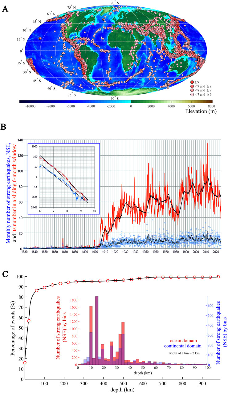
Figure 1. (A) World map of seismic events with magnitudes of 6.0 or greater since 1900, from the USGS ANSS database. The shades of red indicate the earthquake magnitudes (B) Evolution of the global number of strong earthquakes (NSE) over time since 1830, extracted from the USGS ANSS database. The monthly NSE scatter (blue squares) along with its its 6-month average (black line) and sum (red curve) used as input of SSA; NSE in a 5-year window (heavy black line) is shown for informational purposes only. In the inset, the incremental (blue) and cumulative Gutenberg-Richter plots are represented and associated with the following fits: log₁₀N = 7.916–1.100M (R² = 0.973), and log₁₀N = 7.621–1.247M (R² = 0.990), respectively. (C) Distribution of seismic events by depth. The black curve with red circles represents the cumulative percentage of the NSE as a function of depth. The event distribution for the first 100 km is shown in blue for the continents and in red for the oceans, both account for almost 90% of the seismic events. The bins are 2 km width.

The ANSS database contains about 14,000 seismic events from 01 January 1900 to 01 January 2024 with magnitudes greater than or equal to 6. Figure 1B shows a histogram of the number of strong earthquakes over time, with each bin representing a width of 0.5 years. We deliberately start at 1830 to illustrate the evident incompleteness of the database before the 20th century. It should be noted that before installation of the World-Wide Network of Seismograph Stations (WWNSS) in 1960s the list of even strong, magnitude 6.0 or larger earthquakes may be incomplete due to geographically inhomogeneous distribution of then available primarily not standarized seismographs. As a consequence, global studies compiling seismic catalogs (e.g., Engdahl and Villaseñor, 2002; Di Giacomo et al., 2015) suggest that, at the global scale, the catalog reaches completeness around magnitude Mw ∼5.5 from early 60s, while the magnitude completeness is mainly time varying for the first decades of the 20th century, ranging from 6.2 to ∼7.5. To maximize the number of events while maintaining an acceptable level of completeness, we retained earthquakes with magnitudes Mw ≥ 6. This choice is supported by the incremental and cumulative Gutenberg–Richter relation we estimated for the catalog used, whose curve is represented in Figure 1B (inset). To fully preserve the information, we used the complete catalogue (Knopoff and Kagan, 1977; Sornette et al., 1996), including mainshock–aftershock sequences, which are essential to global seismo-tectonic dynamics. This approach also prevents the introduction of artificial temporal variability resulting from declustering, thereby ensuring a rigorous time-series analysis.

The time series of earthquake counts (NSE) was constructed using the number of magnitude M ≥ 6 in a 6-month window sliding by 1-month step. That is, each calendar month is associated with the number of earthquakes that occurred over the preceding 6 months,. This semiannual smoothing reduces short-term fluctuations (e.g., noise from aftershock sequences and therefore indirectly, variability related to distinct tectonic behaviors) while preserving seasonal and inter-annual variations. An annual smoothing window would reduce the 1-year seasonal component, whereas a quarterly window would leave too many irregular fluctuations. The 6-month window represents a good compromise that does not interfere with the detection of cycles longer than 1 year. To ensure the robustness of our analysis, we constructed a median curve using a bootstrap approach (Efron and Tibshirani, 1994; see Supplementary Material) and then analyzed it.

It is also interesting, as a prelude to the mechanism we will propose at the end of our study, to present both the histogram and the cumulative depth distribution of all these earthquakes in Figure 1C, which reproduces the classical observation of Gutenberg and Richter (1954). In black, we plot the cumulative percentage of the number of earthquakes as a function of their depth, which clearly shows that all earthquakes hypocenters fall within 10% of the Earth’s radius from the surface, with almost 90% of earthquakes with magnitude greater than or equal to 6.0 occurring within the first 100 km. If we look closely at the distributions of events down to 100 km (see the red and blue histograms in the same Figure 1C), we see that most of them occurs above 40 km depth, with a median of about 18 ± 10 km. Although this point is well known, it is important to recall it here.

To refine the analysis of the earthquake distribution, we distinguish between earthquakes located in oceanic (red histogram) versus continental (blue histogram) domains based on geographic location of the epicenters relative to coastlines (Figure 1C). It can be observed that the statistics are more or less the same, with the only notable difference being the factor of 2.5 between the number of seismic events under the oceans and on the continents, which ultimately corresponds to the different tectonic modes at plate boundaries.

Finally, for the purposes of our global analysis, we assume that seismicity aggregated worldwide over more than a century may reveal certain stable statistical features common to the entire globe, despite regional disparities and the locally non-stationary nature of seismic processes. In other words, we adopt the working hypothesis that a broad spatio-temporal averaging may allow global-scale modulations to emerge. Nevertheless, we acknowledge that this approach has limitations: in 120 years, the temporal realization of global seismicity has not necessarily sampled all possible variations, and different tectonic regions contribute in uneven ways. Therefore, our study does not assume or assert the strict ergodicity of global seismicity, which is not supported at this timescale.

2.2 Length of day

The length of day (LOD) refers to the duration of a terrestrial day, which is the time it takes the Earth to complete one full rotation on its axis. Although the nominal LOD is set at 24 h, it can actually vary slightly due to various geophysical and astronomical factors. These variations in the LOD are mainly due to the gravitational interactions of the Moon and the Sun, which create tides in the oceans and the Earth’s crust, slowing or speeding up the Earth’s rotation. Mass movements within our planet, such as earthquakes, landslides, shifts in the Earth’s core and changes in the distribution of mass in the oceans and atmosphere, also play a role in these variations. Atmospheric and oceanic effects, such as winds and ocean currents, can also transfer angular momentum to the Earth, changing its rate of rotation (e.g., Melchior, 1958; Gross et al., 1997; Lambeck, 2005; Ray and Erofeeva, 2014; Le Mouël et al., 2019).

Although variations in the LOD are generally very small, on the order of milliseconds, they can be measured with great precision using a combination of modern geophysical and astronomical techniques sensitive to the Earth’s gravitational field, based on observations of stars and satellites such Very Long Baseline Interferometry (VLBI), Satellite Laser Ranging (SLR), and gravimetric measurements (for more details, see Bizouard et al., 2019). Measurements of the variations in the LOD are maintained by the International Earth Rotation and Reference Systems Service (IERS), which produces the EOP14C04 dataset that we have analysed (Figure 2A). This dataset covers the period from 1 January 1962 to 11 March 2024 with a daily sampling interval.

Figure 2

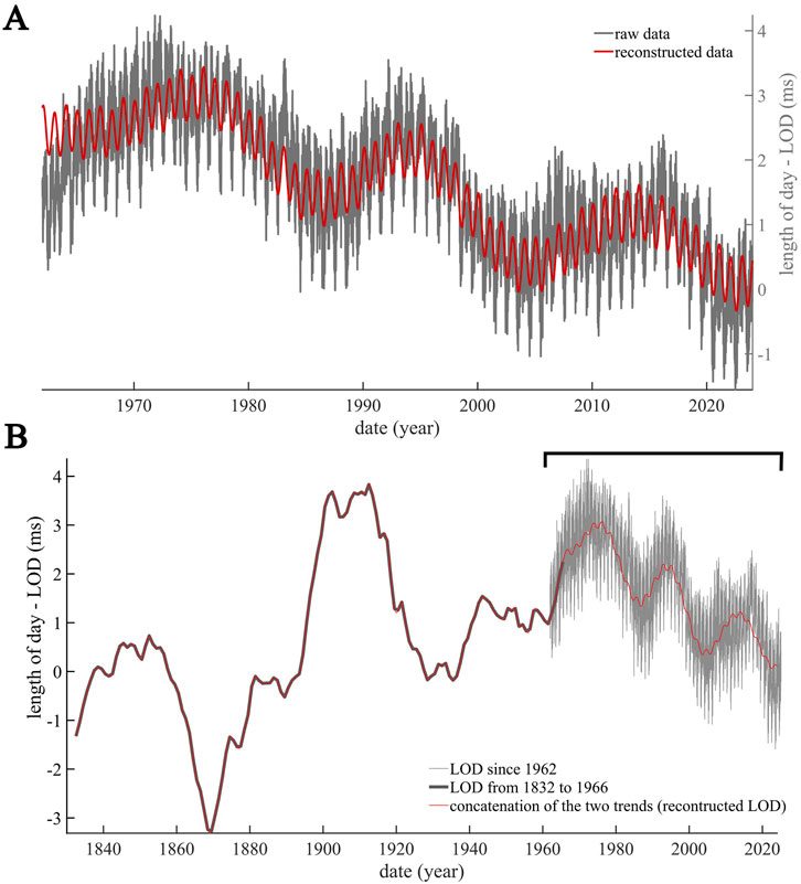
Figure 2. (A) The variation in the LOD (grey curve) provided by the EOP14C04 dataset since 1962. In red, the reconstructed signal based on the main long periods we extracted, e.g., trend, ∼19 years, QBO, ∼1 year, which represents 80% of the original signal. (B) Monthly values of the LOD data (LUNAR97, 1832-1997; represented by the bold black curve) obtained from Stephenson and Morrison (1984) and Gross (2001), alongside daily values (1962-present, represented by the grey curve) provided by IERS. The red curve represents the reconstruction of the LOD time-series since 1832 using the data from Stephenson and Morrison (1984) and Gross (2001) (bold black curve) and the LOD measurements from 1962 made by IERS.

It is, however, possible to extend our analysis further back in time, as other approaches have been used to provide more constraints on the variations in the LOD over past centuries. Thus, for longer durations that are more compatible with the seismic event series (Figure 1), we rely, as in the past (cf. Lopes et al., 2022a), on the compilations of lunar occultation, optical astrometric, and space-geodetic measurements of the Earth’s rotation whose analyses by Stephenson and Morrison (1984) and Gross (2001) resulted in a long LOD time-series which covers the period from 700 BC to 1980 AD. Figure 2B shows the IERS EOP14C04 series from 1962 to the present (grey curve), and the Stephenson and Morrison (1984) series from 1832 (black curve). In red is the concatenation of the low frequency periods, i.e., trend, QBO, 19-year and 1-year periods, extracted from EOP14C04 by Singular Spectrum Analysis (SSA, see section “The pseudo-cycle extraction method”) with periods compatible with the frequency support of long LOD time-series from Stephenson and Morrison (1984) and Gross (2001). Over the ∼20 years of overlap of the long and short LOD time-series, we calculated their average. The red curve (Figure 2B) thus represents the LOD reconstruction since 1832.

2.3 The Brest tide gauge

The Brest tide gauge is unique in that it is both the oldest tide gauge in the world, having been commissioned in 1807 and being still in operation (cf. Wöppelmann et al., 2006; Wöppelmann et al., 2008), and, at the same time, the sea-level trend it records appear to be representative of those observed by all tide gauges in the northern hemisphere (Nakada and Inoue, 2005; Courtillot et al., 2022). Moreover, all these tide gauges show a very similar content of periodic components that is also observed globally, and that is consistent with variations of global pressure data (Courtillot et al., 2022). More, these oscillations are also found in the movement of the mean Earth’s rotation pole (cf. Le Mouël et al., 2021). These observations are most likely due to the particularly stable bathymetry over tens of kilometres of the Breton seafloor (France).

In Figure 3 we have plotted the sea level recorded by this tide gauge, using monthly data (blue curve) provided by the Permanent Service for Mean Sea Level (PSMSL, https://psmsl.org/, PSMSL (2024); Holgate et al., 2013). As can be seen, measurements at Brest were interrupted for some time in the 1840s and 1940s, when the tide gauge was destroyed during the wars.

Figure 3

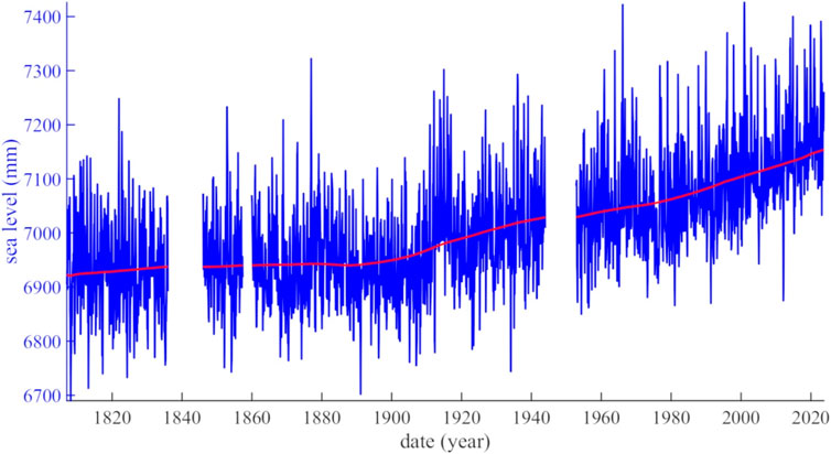
Figure 3. The sea level recorded at Brest since 1807. The data gaps correspond to wartime periods when the tide gauge was destroyed. In blue are the raw data, in red, the mean trend of sea level.

2.4 The Sun, the Moon and the planet’s ephemerides

The ephemerides of the Moon, the Sun and planets are calculated by the Institut de Mécanique Céleste et de Calcul des Ephémérides (IMCCE, https://www.imcce.fr/). We determined, in a geocentric frame, the variations of the positions according to the declination of all the celestial bodies (e.g., Moon, Sun, Jupiter, Saturn, etc.).

2.5 The pseudo-cycle extraction method

The data we analysed are not necessarily stationary in the strict sense, which may be expected considering the nature of the phenomena, and can sometimes be discontinuous, as is the case for the sea level in Brest. We therefore need a sufficiently robust method to extract pseudo-cycles. By pseudo-cycle we mean an oscillation that can be highly modulated in both phase and amplitude, but whose Fourier spectrum, although spread around a nominal frequency, remains exclusively centred around that frequency. Singular Spectrum Analysis (SSA) is an ad hoc decomposition method, i.e., the orthogonal basis on which the signal information is projected and is constructed from the information of the signal itself (unlike the infinite sines of the Fourier transform, for example,), which makes it particularly well suited to this problem (cf. Vautard and Ghil, 1989; Vautard et al., 1992).

We have already described the SSA algorithm in Lopes et al. (2022b), and it is even the subject of a reference work by Golyandina and Zhigljavsky (2013), which details all its possible variations. In the present paper we briefly outline the main aspects of the method, while more details can be found in the Supplementary Material. It consists of four steps. In the first, embedding step, the data are projected into a specific matrix X, either a Toeplitz matrix or a Hankel matrix (cf. Lemmerling and Van Huffel, 2001). Essentially, a segment of the signal of length L is written in each column of the matrix X. The value of L determines the physical properties (e.g., chaotic, strange attractor, short or long period, etc.) that will be extracted from the data. The second step consists in diagonalising the previously matrix built X, typically by Singular Value Decomposition (SVD, Golub and Reinsch, 1971), which yields two matrices of eigenvectors inducing a passage from the data to the dual space (thus an ad hoc orthogonal basis), with the eigenvectors sorted in descending order of the corresponding eigenvalues. These latter are eigenvalues of the autocorrelation matrix XX^T, which makes that they correspond by definition to the variance (Lopes et al., 2024). This is analogous to a Fourier spectrum. In the third step, known as the grouping step, similar or close eigenvectors and eigenvalues are paired, known as the grouping step. Finally, in the last step, called Hankelization, the grouped eigenvector/eigenvalue pairs are returned to the data space. That is how the pseudo-cycles that correspond to these pairs are extracted and reconstructed. We calculated their uncertainties using their spectra width at half peak’s maximum. For each component extracted in the different geophysical time-series, we calculated the associated variance. This latter corresponds to the square root of the sum of the squares of the eigenvalues that comprise the component. We refer to the total variance or total energy (of the originial signal) when calculating the sum of selected eigenvalues. This can be viewed as an analogous to a coefficient of determination (R²), reflecting the goodness-of-fit of the decomposition.

Regarding the time-series analysis applied on seismic data, one must keep in mind that the earthquake catalog is not uniformely complete, especially for magnitudes above 6, for the time period from 1900 to 2024 (e.g., Engdahl and Villaseñor, 2002; Kossobokov, 2006; Kossobokov and Nekrasova, 2018) as previously highlighted with the magnitude completeness. However, we are studying the number of strong earthquake as a scalar at the planetary scale. Thus, the associated error remains consistent over time and across locations, which tends to be reduced over recent time due to instrumentation increase. Therefore, the shapes of variations and pseudo-periodicities detected and extracted in a detrended signal should be similarly affected, allowing us to perform a reliable analysis. On the contrary, the slowly-varying trend (Supplementary Material, Supplementary Figure C2) which is not further interpreted in this study, reflects mainly but not exclusively this inventory-growth bias.

3 Results and descriptions of the analysed signals

The main long-period pseudo-cycles (≥1 year) that we have detected and extracted are shown in Supplementary Material (Sections C to E); the trend is only shown NSE (Supplementary Figure C2). The analysis highlights the coincidence of 7 cycles between the NSE and the LOD, and four cycles with the variation of the SL@B (Table 1). These pseudo-cycles are, in ascending order: the 1-year seasonal oscillation the 2.3-year Quasi-Biennial Oscillation (QBO, Baldwin et al., 2001), a ∼11-year pseudo-cycle that may have a connection with Jupiter’s orbit, except for the SL@B, where it was absent–unlike in the mean global sea level, e.g., Courtillot et al. (2022); Le Mouël et al. (2021); Lopes et al. (2021) – a ∼14-year pseudo-cycle (periodicity related to Jupiter + Uranus, Scafetta and Bianchini, 2022), a ∼19-year pseudo-cycle corresponding to the precession of the lunar orbit which has an (exact) period of 18.6 years, a ∼33-year pseudo-cycle, and finally a ∼65 years pseudo-cycle. In Supplementary Figures C3-C7, D1-D5, E1–E4, we illustrated some of these pseudo-oscillations and their reconstruction for the three time-series analyzed. The reconstruction of the extracted pseudo-periods shows that the sum of these cycles corresponds to about 88% of the NSE, about 89% of the variation in the LOD and about 90% of the variation in the SL@B. These pseudo-periods are summarised in Table 1. One can note the high levels of uncertainty in the determination of long-term cycles: for the∼33-year cycle, a factor about 1.3 between the NSE and the SL@B, and similarly, a factor of 0.4 for the ∼60-year pseudo-cycle. In the following, we present the common cycles extracted in the three geophysical time-series. These detected multi-decadal components (∼33 years and ∼60 years) should be interpreted with caution, given the greater uncertainties due to incomplete data at the beginning of the record.

Table 1

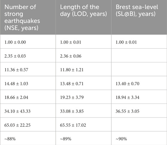
Table 1. Summary of pseudo-periods detected and extracted from three geophysical datasets, i.e., NSE, LOD, and SL@B. The last line indicates the percent of signal reconstructed using the listed cycles.

3.1 The seasonal oscillation

Figure 4A shows the seasonal pseudo-cycle extracted from the three geophysical datasets. The time axis starts from 2000 for better readability of the observations. As we can see, the variations in the SL@B (blue curve) and the NSE (red curve) are in perfect phase quadrature (±φ/4), which corresponds to a temporal derivative, with the variations in the LOD. Once this phase shift is applied, all curves overlap almost perfectly (Figure 4B).

Figure 4

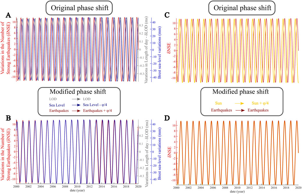
Figure 4. The seasonal oscillation. (A, B) The ∼ 1-year pseudo-cycle extracted by SSA since 2000 for better readability, from the NSE (red curve), LOD (grey curve) and SL@B (blue curve). (C, D) The ∼1-year pseudo-cycle extracted from the NSE (red curves) superimposed on the same component but extracted in the ephemeride of the Sun (yellow curve). In (A) and (C), the original phase shifts extracted by SSA are shown; in (B) and (D), the same curves as in (A) and (C) respectively, are phase shifted by one quadrature (±φ/4) for the NSE and SL@B in (B), and the Sun (D).

In Figure 4C we have superimposed the ephemeride of the Sun (yellow curves) on the annual variation in the NSE over the same period. A phase quadrature is clearly visible, similarly as between the SL@B and NSE and LOD (Figures 4A,B) which, when applied to the envelope, perfectly matches the geophysical observations (cf. Figure 4D).

3.2 The quasi-Biennial oscillation

As mentioned above, we have not identified the QBO in the SL@B, but this does not mean that it does not exist in general. In Figure 5, we show the excellent agreement between the periods of the QBO extracted in the NSE (red curve) and the QBO from the LOD measurements (grey curve). Clearly, over the period of interest here, i.e 1962 to 2024, which coincids also with the period of the improved earthquake hypocenter determinations after installation of WWNSS, the phase variation between the two geophysical parameters does not appear to be constant, as was the case for the forced seasonal oscillation (see Figure 4). For this reason, we have evaluated and plotted the evolution of the instantaneous phase shift over time in Figure 5B. As we can see, we start in 1962 with an almost perfect phase opposition between the two geophysical measurements and arrive in 2024 to a simple quadrature.

Figure 5

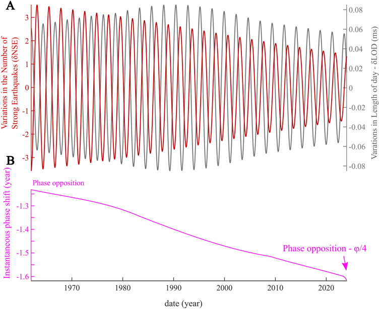
Figure 5. The Quasi-Biennial Oscillation (QBO) of ∼2.3 years. (A) The QBO extracted from the NSE (red curve) is superimposed on the QBO extracted from the LOD (grey curve). (B) The evolution of the instantaneous phase shift since 1962; over 60 years, a phase opposition transitions to a phase quadrature (∼-φ/4).

3.3 The ∼11-year pseudo-cycle

It has long been known that one of the most significant pseudo-cycle components in the LOD occurs at a period of about 11 years (cf. Stephenson and Morrison, 1995; Le Mouël et al., 2019), and might well express the influence of Jupiter. This pseudo-cycle has also been identified in the polar motion (cf. Lopes et al., 2017), although its amplitude is more modest. Surprisingly, it is found only occasionally and modestly (e.g., Currie, 1981) or not at all (cf. Courtillot et al., 2022) in the global mean sea level, which may seem paradoxical when considering the mechanisms that should accelerate or decelerate the Earth’s rotation according to Laplace’s theory (Lopes et al., 2021).

We have extracted the 11-year pseudo-cycle from the NSE and plotted it in Figure 6A (red curve). In Figure 6B, we have shifted the seismic oscillation by one phase quadrature, as we did previously in Figure 4B for the seasonal pseudo-cycle. Once again, the two curves, LOD and NSE, are in phase. In Figures 6C,D we compare the Jupiter ephemerides (pink curve) with the seismic pseudo-cycle, and again the phase match is perfect once the quadrature shift is removed.

Figure 6

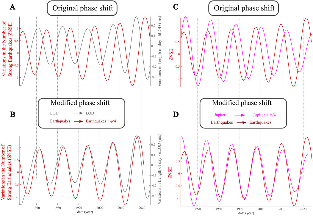
Figure 6. The ∼11-year pseudo-cycle. (A, B) The ∼11-year oscillation detected and extracted from the NSE (red curve) and LOD (grey curve) since the 1960s. (C, D) The same pseudo-cycle (red curves) superimposed on the same component but extracted in the ephemeride of Jupiter (purple curve). In (A) and (C) are shown the original phase shifts, in (B) and (D) are the same curves as in (A) and (C) respectively, but phase shifted by one quadrature (±φ/4).

3.4 The ∼14-year pseudo-cycle

Unlike previous cycles, this one shows significant phase modulation on a century scale (Figure 7A). Seismic activity (NSE) and SL@B, which are almost in phase during the 120 years of observation, were in phase with the reconstructed LOD at the beginning of the last century, and reached a phase opposition only by the mid-2010s (Figure 7A). This consistent phase shift may have several causes, but it is most likely that the primary cause taking place at this time scale is that the extracted frequencies are slightly different (see the associated uncertainties in Table 1), although their associated spectral widths make them compatible. An interesting observation is that the amplitude modulations between seismic activity and sea level also appear to exhibit an inverse correlation over the entire period.

Figure 7

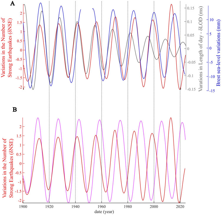
Figure 7. The ∼14-year pseudo-cycle. (A) The 14-year oscillation extracted from the three geophysical data sets without phase shifting with in red that of the NSE, in blue the SL@B and the reconstructed LOD in grey; (B), we reported the same component of the NSE (red curve), together with that extracted from the ephemerides of Jupiter and Uranus (purple curve).

The planetary commensurability corresponding to this period is generally attributed to the Jupiter + Uranus pair (cf. Scafetta and Bianchini, 2022). We have superimposed the evolution of this commensurability (Laplace’s resonnance) using the ephemerides of the two aforementioned planets (purple curve) on the curve of the NSE (red curve) in Figure 7B. A good agreement can be observed during the period 1900-1950, after which the gradual phase shift between the two physical phenomena becomes more pronounced, and since the early 2000s the two curves are in phase opposition.This transition might result from the aforementioned revolutionary change in earthquake determinations in the 60s (see subsection Earthquake data).

3.5 The 18.6-year lunar pseudo-cycle

The ∼19-year pseudo-period detected and extracted from the three geophysical records corresponds to the 18.6 years oscillation, which, as mentioned above, is caused by the precession of the lunar orbital plane. Figure 8A shows the corresponding curves. As in the case of the annual oscillation (cf. Figure 4A), the SL@B and NSE are both in phase quadrature with the variations in the LOD. Once this phase quadrature is applied, all geophysical records are almost perfectly in phase (cf. Figure 8B). The ephemeride of the Moon (green curve) and the NSE (in red) in Figure 8C are almost perfectly in phase, when we shift it by a phase quadrature (Figure 8D).

Figure 8

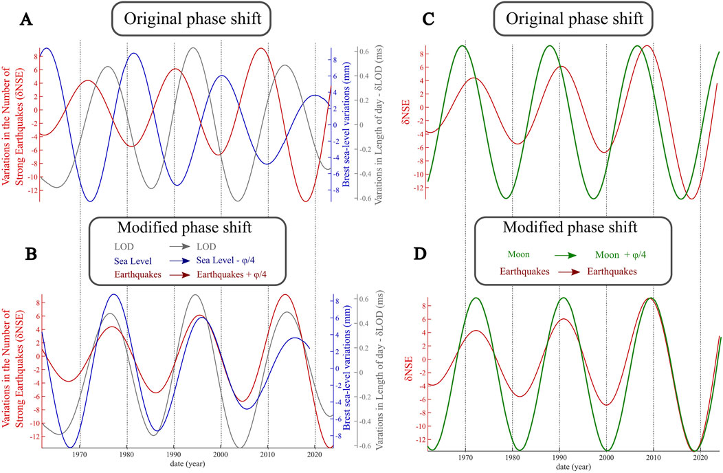
Figure 8. The 18.6 years pseudo-cycle. (A, B) The ∼19-year component extracted in the NSE since 1962 (red curve), LOD (grey curve) and the SL@B (blue curve). (C, D) The ∼19-year component extracted in the NSE (red curve) represented together with that extracted from the Earth-Moon distance (green curve). In (A) and (C) are shown the original phase shifts, in (B) and (D) are the same curves as in (A) and (C) respectively, but phase shifted by one quadrature (±φ/4).

3.6 The ∼33-year pseudo-cycle

Although SSA is more robust for extracting components than, for example, wavelet methods, it is of course not perfect. As shown in Supplementary Figure E1 for the Brest tide gauge analysis, data gaps lead to edge effects on the waveforms that are not insurmountable, but still present. To avoid misinterpretation due to these edge effects, Figure 9A shows the superposition of the 33-year pseudo-cycles of the reconstructed LOD (grey curve) and seismic events (red curve) since 1900. A phase opposition appears which, when applied to seismicity, results in an almost perfect superposition of the two geophysical records (Figure 9B). Figures 9C,D show the same curves but starting in 1958, which is the beginning of the last continuous segment of the Brest tide gauge record. Thus, in Figure 9C, we have added the 33-year oscillation of SL@B (blue curve) to the two previous geophysical records. Again there is a phase opposition with the reconstructed LOD which, when removed from the SL@B, allows a good superimposition of the three geophysical records (Figure 9D).

Figure 9

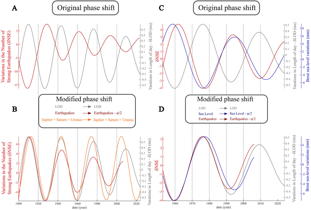
Figure 9. The ∼33-year pseudo-oscillation. (A, B) The 33-year component extracted from the NSE since 1900 (red) and from reconsructed LOD (grey). In (B), the ephemerides of the combination Jupiter + Saturn + Uranus was added. (C, D) Same component but shown from 1958, for three geophysical time-series: the NSE (red), the SL@B (blue) and the reconstructed LOD (grey). In (A) and (C) are shown the original phase shifts, in (B) and (D) are represented the same curves, but phase shifted by one phase opposition (±φ/2).

One can note that this 33-year cycle is also found in sunspots (e.g., Usoskin, 2017; Le Mouël et al., 2020) and corresponds to one of Laplace’s commensurable ratios between Jupiter, Saturn and Uranus (e.g., Mörth and Schlamminger, 1979). Despite these observations, it is important to keep in mind that this ∼33-year pseudo cycle, is one of those that are less reliable, with the ∼60 years. It is the unique long oscillation with uncertainties larger than the periodicity itself (Table 1).

3.7 The ∼60 years pseudo-cycle

Regarding this last pseudo-cycle of ∼60 years, whose determination is less reliable if we consider the associated uncertainties (Table 1), we did not detect it in the Brest sea level data (SL@B), which does not necessarily mean that it does not exist, since we know that it clearly appears in the global mean sea level, with a period of 57.5 ± 7 years (Courtillot et al., 2022). As for its correspondence with ephemerides or commensurabilities, one can note that this cycle corresponds to the Uranus + Neptune pair (Table 2), although this observation should be taken with caution. Only barely two cycles have been observed since 1900 (Figure 10), and like the trend–which we have not addressed here, one cannot reasonably say more than that the ∼60 years pseudo-cycle is found in the mean sea level, the mean seismicity and the reconstructed LOD.

Table 2

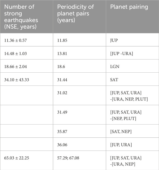
Table 2. List of periodicities extracted from the time-series NSE common to LOD (see Table 1). The last two columns indicate the combination of planet pairing and the associated periodicities as reported in Courtillot et al. (2021), Lopes et al. (2021) as well as Scafetta and Bianchini (2022). The planets are listed as follows: JUP for Jupiter, NEP for Neptune, PLU for Pluto, SAT for Saturn, URA for Uranus. LGN stands for lunar great nutation. The brackets separate different pairing.

Figure 10

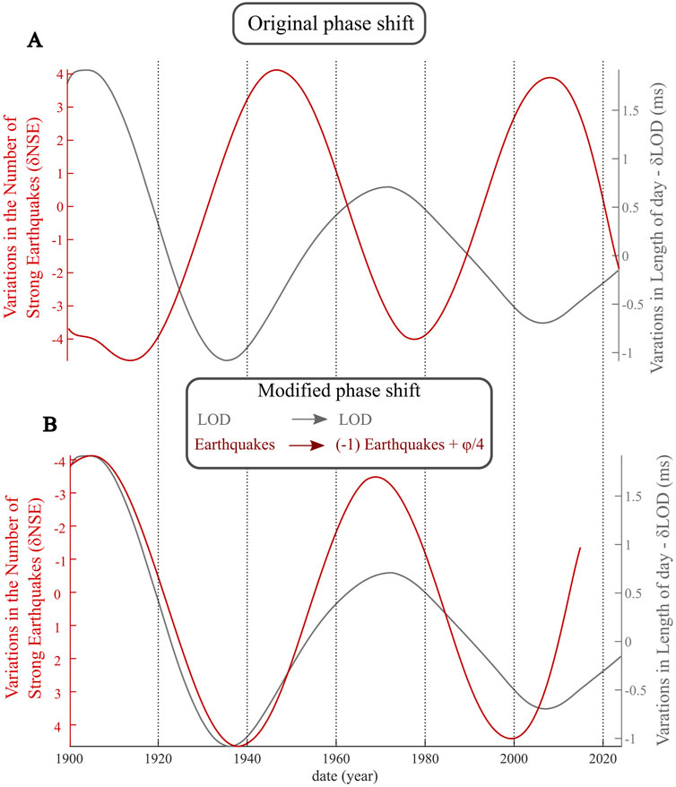
Figure 10. The ∼60-year pseudo-cycle, with the reconstructed LOD (grey curve) and NSE (red curve) shown (A, B). In (B), the same curves are realigned by a phase quadrature.

In summary, 6.0 of the seven pseudo-cycles detected and extracted, are in perfect quadrature or opposition and they appear in the ephemerides of the Moon, Sun and the main planets of our solar system (Table 2), which are known to influence the rotation of the pole (Lopes et al., 2021). Moreover, it is the first time that the QBO, which is not in quadrature nor in opposition, has been unambiguously detected and extracted from global seismicity.

4 Discussion

4.1 On the periodicities detected

By performing a comparable time-series analysis on three fundamentally different geophysical datasets, differing in both physical nature and data characteristics, we aimed at evaluating and identifying potential common external forcings modulating the distinct phenomena that are the Earth’s rotation, the water-mass movements, and the seismic activity. While the cyclic behavior of the parameters of the Earth’s rotation and the hydropshere were already known, our investigation revealed the existence of periodic components, in the NSE over an interval of 124 years, starting in 1900. We detected seven cycles, spanning interannual to decadal periods, common to those present in the polar motion, and more specifically in the LOD; four of them, being also present in the sea-level (Table 1). These observations align with studies claiming that intermediate and strong earthquake occurrence appears to follow lunisolar tidal cycles for short periods (Lockner and Beeler, 1999; Métivier et al., 2009; Petrosino et al., 2018; Varga and Grafarend, 2019; Lordi et al., 2022; Zuddas and Lopes, 2024), and solar activity for longer ones (Simpson, 1967; Mazzarella and Palumbo, 1989; Choi, 2010; Marchitelli et al., 2020).

Among the periodicities detected in Table 1, that of ∼11 years is a well known cycle of the solar activity, that has been largely recorded in terrestrial phenomena such climate (Currie, 1984; Currie and Fairbridge, 1985; Scafetta, 2021), sea and groundwater level (Zhou and Tung, 2010; Liesch and Wunsch, 2019; Diodato and Bellochi, 2024; Fan et al., 2024; Courtillot et al., 2022), and magnetic field (Le Mouël et al., 2019). A correlation has also been made by several authors between this decadal solar cycle and seismic activity (Mazzarella and Palumbo, 1988; Marchitelli et al., 2020; Takla and Samwel, 2023) but also in volcanic activity (Le Mouël et al., 2023 and references therein), however most of these results have been highly debated due to lack of credible physical mechanism. One can note that this periodicity matches also well with the orbital period of Jupiter (∼11.86 years), which has been associated with modulations in the solar activity and motion (Scafetta, 2020; Courtillot et al., 2021; Lopes et al., 2021). Interestingly, this cycle as well as the six other pseudo-periods we identified in the NSE are known as commensurable periods corresponding to specific orbital configuration (Table 2), e.g., alignment or quadrature of individual or paired planets of the Solar system (Mörth and Schlamminger, 1979; Courtillot et al., 2021; Lopes et al., 2021; Scafetta and Bianchini, 2022). All of these cycles have not only been detected in the Earth’s geodynamics (this study, Le Mouël et al. (2023) and references therein) but also in the other dynamical fluid envelopes of our planet, namely, the atmosphere and hydrosphere (for the 60-year cycle: Mazzarella and Scafetta, 2012; the ∼30years cycle; Liesch and Wunsch, 2019; de Vita et al., 2012). The period of 18.6 years which relates to the Earth’s satellite, corresponds to the longest lunar period, the Great Lunar Nodal Cycle, similalry modulates ocean and atmosphere (Currie, 1984; Currie and Fairbridge, 1985; O'Brien and Currie, 1993; Herweijer et al., 2007; Le Mouël et al., 2019) in addition to solid Earth and appears in lod (Le Mouël et al., 2019).

Detecting these periodicities in various geophysical phenomena is consistent with the hypothesis of an external forcing acting globally across the Earth. Moreover, spectral analyses conducted separately for oceanic and continental earthquakes reveal very similar dominant periodicities, suggesting that the observed modulations are global in nature and transcend local tectonic contexts (Supplementary Material, Supplementary Figure C1). This hypothesis of the origin of these periodicities is also supported by the obervations we made in terms of modulation in phase and amplitude of the extracted periodicities. Thus, the phase lag of φ/4 – φ the cycle, was observed between (i) most of the components extracted in the three geophysical time-series studied, e.g., the NSE, SL@B and LOD, on one hand, and (ii) in a component of the polar motion or specific planetary ephemerides, on the other hand (Figures 2–10). If local processes would have dominated the response of faults to these long oscillations, such phase lag would likely not have been consistent and maintained over time, and in particular, it would likely not be the same for the different periods extracted, due to local conditions (pore-fluid pressure, stress field, etc.), as well as the heterogeneity in the internal properties (composition, porosity, permeability, etc.) of rocks composing the Earth’s lithosphere. Similarly as for the results obtained for the analysis of the global volcanism (Le Mouël et al., 2023), the phase lag of φ/4 which represents a shift related to temporal derivative of sinusoidal functions, was detected between the solid Earth and fluid envelopes on one hand, and the polar motion on another hand. These results are coherent with Laplace’s theory in which, the time shift expresses a causal chain of forces acting in response to orbital moments of the Jovian planets (Lopes et al., 2021; 2022a; Le Mouël et al., 2023; Figure 9). In addition to these observations, we would like to draw attention to the pseudo-cycles we extracted in this present study, they are characterized by periods and waveforms that are more than compatible to even identical with those we had discovered in global volcanism (Le Mouël et al., 2023; Figure 11), again independently of the nature of the eruption and the volcano setting. Moreover, a series of papers have demonstrated that probable similar forcing participate in the same way, in the triggering of volcanic eruptions, driven by variations in the sea level on long-term, (as shown in this study, Dumont et al., 2022; 2023; Satow et al., 2021), or on short-term, through a tidal modulation of the magmatic and hydrothermal fluids (De Lauro et al., 2013; Dumont et al., 2021; Petrosino and Dumont, 2022).

Figure 11

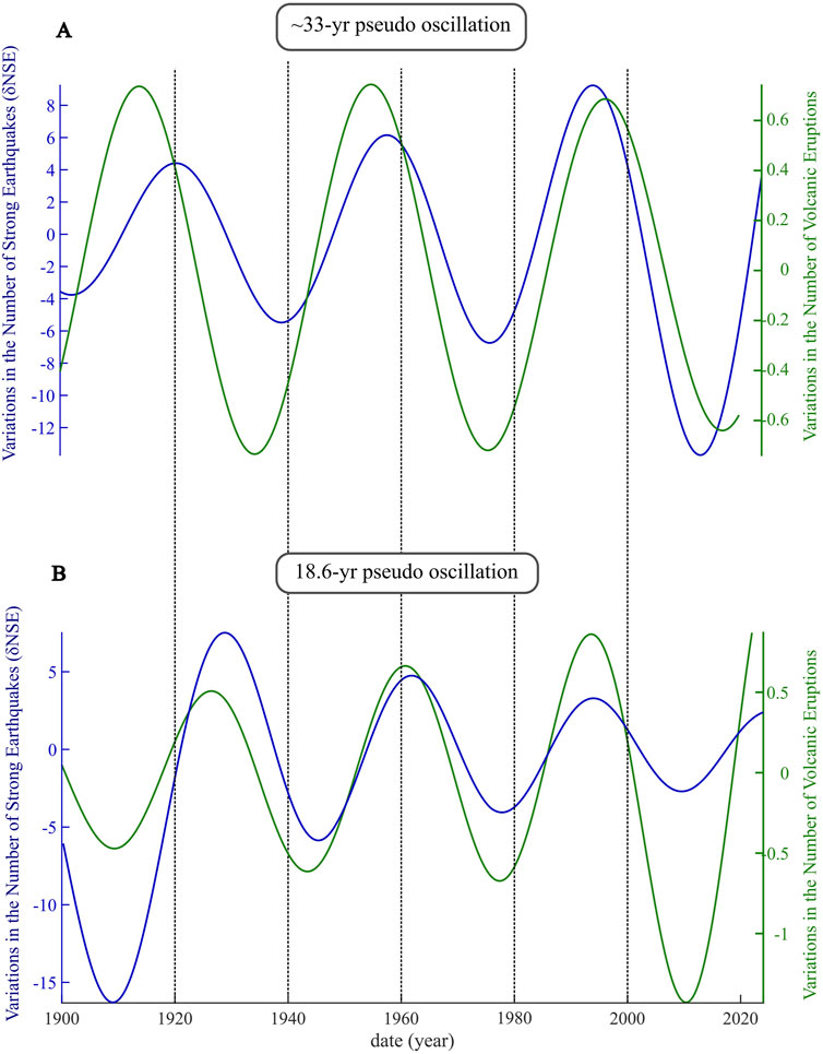
Figure 11. Comparison between the ∼33-year period (A) and the ∼19-year period (B) pseudo-cycles extracted from the global series of volcanic eruptions (green) (from Le Mouël et al., 2023) and the global series of strong earthquakes (blue, the present study).

4.2 On the possible trigger mechanism

The planetary-scale forcing hypothesis proposes that the triggering of global strong earthquakes results from the transfer of energy via angular momentum exchanges, in a similar way as proposed by previous studies for other processes taking place on Earth (Courtillot et al., 2021; Lopes et al., 2021; Le Mouël et al., 2023). Such planetary forcing should be able to influence in one way or another rock failure. However, external gravitational influences, being extremely weak, are unlikely to trigger major earthquakes on their own; the strongest tides on Earth, that are of lunisolar origin, are associated with tidal stresses that are two to four orders of magnitude lower than the strength of rock and faults (∼10¹–10³ MPa, Scholz, 2019). The influence of other planets of our solar system is therefore weaker than lunisolar ones, raising the question on how such interaction can occur. Yet, they might play a secondary role in modulating the timing of rupture in faults that are already critically stressed, by subtly altering stress conditions, fluid pressures within the Earth’s crust or destabilisation of the rock matrice. We thus propose a scenario of indirect forcing: planetary angular momenta by affecting global parameters such as Earth’s rotation and ocean mass distribution, could exert a slight but sufficient influence on the crustal stress regime, potentially advancing or delaying the occurrence of earthquakes under specific conditions. In this hypothetical scenario, we put forward the role of crustal fluids as explain further below.

Earthquake triggering is as an intricate process reflecting the complexity of physico-chemical processes taking place in the Earth’s heterogeneous lithosphere (Keilis-Borok, 1990; Tamburello et al., 2018), i.e., a hierarchical structure of blocks-and-faults extending from the scale of tectonic plates to that of grains of rock minerals. Earthquakes can be regarded as a critical transition of such non-linear complex systems. Similarly, the Earth’s network of faults may be seen as a metastable system whose instability reflects a stored energy originating in physical and/or chemical mechanisms like for instance, the Rehbinder effect in materials science (Gabrielov and Keilis-Borok, 1983; Traskin, 2009), whereby fluids or chemical agents can weaken discontinuity surfaces and facilitate rupture (Miller 2013; Pampillón et al., 2023), non-linear filtration (Barenblatt et al., 1983), “fingers” springing out at the front of a migrating fluid (Barenblatt, 1996), sensitivity of dynamic friction to local environment (Lomnitz-Adler, 1991), release fluids, and much more. Many of the aforementioned mechanisms involve fluids which are ubiquitous to our planet and are known to participate in rock failure by reducing effective stresses within the material (Gabrielov and Keilis-Borok, 1983; Scholz, 2019; Wang and Manga, 2021; Kocharyan and Shatunov, 2024; and therein references).

Hydrochemical studies of groundwater provide significant insights into fluid–rock interactions, which lie at the heart of the mechanism we propose. It is important to consider that not all minerals are in thermodynamic equilibrium with water under the conditions of groundwater stored in the Earth’s crust. Groundwaters can be thus seen as an evolutionary system allowing the thermodynamic balance between unstable and newly-formed yet stable mineral phases by promoting dissolution-precipitation processes (Zuddas, 2010). This mainly leads to changes in water content, reflected in ion balance and composition (major elements, electrical conductivity), CO₂ release, redox conditions, pH levels, and variations in stable isotopic ratios such as ³He/⁴He (Perez et al., 2008; Reddy and Nagabhushanam, 2012; Skelton et al., 2014; 2019; Barberio et al., 2017; Buttitta et al., 2020; Chiodini et al., 2004; 2020; Di Luccio et al., 2022; Zuddas and Lopes, 2024). These changes, in turn, affect mineral surfaces and rock properties, especially porosity and permeability, which may affect the internal stability of rock. Recent studies in North Iceland have shown that water content variations in basaltic rocks can precede earthquakes (M > 5) by up to 6 months, enabling retrospective forecasting based on a decade of data (Skelton et al., 2019; 2024). These findings suggest that (1) rock destabilisation can be critically detected months before a large seismic event, (2) fluid-rock interactions participate in rock weakening and microfracturing, (3) such processes affect not only carbonates, but also silicates and (4) they occur over short timescales. Zuddas and Lopes (2024) further show that tidal forces may mechanically drive groundwater movement, enhancing CO₂ release through water-rock interactions, in addition to mantle emissions (Chiodini et al., 2020). Faults, as complex fluid pathways, provide extensive surfaces for dissolution-precipitation reactions that weaken or seal rock structure (Kocharyan and Shatunov, 2024). This makes them more susceptible to rupture under even low-amplitude, long-term oscillations, such as interannual to decadal variations highlighted in this study.

One can note that the dissolution process is a complex and non-linear phenomenon, so we cannot expect seismicity in a given region to respond directly to extraterrestrial forces. However, over long periods and from a global perspective, there is no reason to rule it out, and this is what our analysis indicates. This interaction would thus have two primary consequences: mineral dissolution, which weakens the ground, and the release of gases. Our study provides no direct evidence for the involvement of fluids, thus further works are necessary for testing and validating this hypothesis, requiring long and high resolution time-series of hydrochemistry and gas emissions such those performed in Italy (Barberio et al., 2017; Buttitta et al., 2020; Chiodini et al., 2004; 2020; Di Luccio et al., 2022) or in Iceland (Skelton et al., 2014; 2019).

If the mechanism we suggest will be further confirmed, it should also play a role in volcanic eruptions. Volcanic environments, in addition to also host groundwater, are usually associated with hydrothermal systems which are recognized to be of critical importance in what deals with the system stability (Heap et al., 2021). In Figure 11, we superimpose the ∼33-year and the ∼19-year components extracted in the global volcanism (data from Le Mouël et al., 2023) and the corresponding components extracted in the NSE, revealing a strong in-phase correlation.

4.3 On the limits

Our appraoch based on the identification of periodic components common to different physics and in particular, related to the various Earth’s envelopes led us to assume an indirect forcing between the global strong seismicity on Earth and ephemerides. The identification of each cycle from diffent geophyscal time-series took into account their uncertainties. Moreover, for most of these pseudo-cycles, we observed a phase or phase opposition link once a delay of ± φ/4 was applied. One can note that this phase relation was globally well maintained over the 124-year interval, but for a few case, typically the 14-year and 2.3 years pseudo-cycles (Figures 5, 7), a varying phase lag could be observed. This effect is mainly related to the different uncertainties associated with the compared oscillations. Physically, and considering and indirect coupling, these phase lags could also represent a delay in the response of the causal chain which first affect the Earth’s roration axis motion (Lopes et al., 2021; Le Mouël et al., 2023), and whose lagged response could express a combined effect of various processes related to Earth’s inertia, viscoelastic relaxation within the Earth’s interior, but also the transfer through intermediate variables (e.g., fluid redistribution).

Despite covering 124 years, the seismic catalog used in this study is notably incomplete during the early decades, especially before ∼1940. This limitation is more likely to affect the detection of long-period oscillations (e.g., ∼30–35 and ∼60 years) than shorter cycles (1–∼19 years), which are better resolved due to their more frequent repetition within the observation window. This is reflected in the uncertainty estimates: longer-period components exhibit significantly larger uncertainties—sometimes exceeding the amplitude of the oscillation itself, as in the case of the ∼33-year cycle (Table 1). Interestingly, both the ∼33- and ∼60-year oscillations appear stronger in the early 20th century and weaken thereafter, a pattern consistent with improving catalog completeness. Missing events in earlier decades could exaggerate apparent fluctuations due to their disproportionate weight in a sparse dataset. Alternatively, the amplitude of external forcing—or the seismic system’s sensitivity to it—may itself vary over time, though this cannot be resolved with the current data. Accordingly, we avoid overinterpreting these long-period modulations, despite parallels in climate and planetary literature (e.g., the ∼179-year Jose cycle and its ∼60-year harmonic; Chen et al., 2004; Valdés-Pineda et al., 2018; Mazzarella and Scafetta, 2012). Longer-term records or improved historical catalogs will be necessary to confirm whether these cycles are persistent features or artifacts.

While we observe temporal coincidences between certain seismic pseudo-cycles and astronomical cycles, it is important to emphasize that the primary driver of earthquakes remains the accumulation of tectonic stress at plate boundaries. Thus, these periodicities could also reflect, at least in part, poorly understood internal Earth dynamics. The Gutenberg-Richter law, along with the stochastic nature of earthquake occurrences, implies that part of the observed variability in strong earthquakes could be coincidental or the result of intrinsic noise as well as complexity including dynamical behavior of the seismic system (Turcotte and Malamud, 2002; Sobolev, 2011; Rodriguez Piceda et al., 2025).

5 Conclusion

With this study, we aim at examining the temporal evolution of the global seismicity, focusing on the earthquakes of magnitude 6.0 or greater since 1900, in order to identify a common feature that might help us to deduce and propose a new general trigger mechanism. First, we present the dataset of seismic events (NSE) from 1 January 1900 to 1 January 2024, detailing its spatial distribution and general statistics. Next, we introduced two time-series related to tidal influences on Earth, specifically the LOD variations and sea level records from Brest, the latter being a representative gauge for general ocean levels, particularly in the Northern Hemisphere. These three series were decomposed via SSA, revealing that they can be represented as the sum of seven quasi-periodic components related to the planetary commensurabilities of major Jovian planets, as well as the Sun, and the Moon. Altogether, these periods account for ∼88% of the total energy in the seismic events signal, ∼89% of the LOD variations, and 90% of the sea level fluctuations at Brest (SL@B). They include, the annual oscillation, the Quasi-Biennial Oscillation (QBO), the ∼11-year, the ∼14-year, the ∼19-year, the ∼33-year, and finally, the ∼60-year pseudo-cycles, all known to manifest across various geophysical phenomena. We show that they are mainly in phase quadrature (i.e., $\frac{φ}{4}$ ) with planetary ephemerides. This constant, precise phase shift evokes Laplace’s equations in global mechanics, in which the hydrosphere is known to oscillate in quadrature with LOD variations. We discuss our results in the context of hydro-lithosphere interactions, focusing on water-rock interactions that reconcile both physical and chemical processes as well as the matter of scale.

Data availability statement

Publicly available datasets were analyzed in this study. This data can be found here: https://earthquake.usgs.gov/earthquakes/search/; https://www.iers.org/IERS/EN/DataProducts/EarthOrientationData/eop.html; https://psmsl.org/; https://www.imcce.fr/.

Author contributions

SD: Writing – review and editing. JdBd’A: Writing – review and editing. J-BB: Writing – review and editing. VC: Writing – review and editing. MG: Writing – review and editing. DG: Writing – review and editing. VK: Writing – review and editing. J-LL: Writing – review and editing. FL: Writing – review and editing. MN: Writing – review and editing. GS: Writing – review and editing. SP: Writing – review and editing. PZ: Writing – review and editing.

Funding

The author(s) declare that financial support was received for the research and/or publication of this article. This work was supported by the Portuguese Fundação para a Ciência e Tecnologia FCT I.P./MCTES through national funds (PIDDAC) – UID/50019/2025 (https://doi.org/10.54499/UIDP/50019/2020), LA/P/0068/2020 (https://doi.org/10.54499/LA/P/0068/2020), and FCT-through project RESTLESS (PTDC/CTA-GEF/6674/2020, http://doi.org/10.54499/PTDC/CTA-GEF/6674/2020).

In Memoriam

Marc Gèze passed away before the finalization of this manuscript. We dedicate this work to his memory.

Conflict of interest

The authors declare that the research was conducted in the absence of any commercial or financial relationships that could be construed as a potential conflict of interest.

The author(s) declared that they were an editorial board member of Frontiers, at the time of submission. This had no impact on the peer review process and the final decision.

Generative AI statement

The author(s) declare that no Generative AI was used in the creation of this manuscript.

Publisher’s note

All claims expressed in this article are solely those of the authors and do not necessarily represent those of their affiliated organizations, or those of the publisher, the editors and the reviewers. Any product that may be evaluated in this article, or claim that may be made by its manufacturer, is not guaranteed or endorsed by the publisher.

Supplementary material

The Supplementary Material for this article can be found online at: https://www.frontiersin.org/articles/10.3389/feart.2025.1587650/full#supplementary-material

Footnotes

¹https://earthquake.usgs.gov/earthquakes/search/(USGS Earthquake Hazards Program, 2017)

References

Albini, P., Musson, R. M., Rovida, A., Locati, M., Gomez Capera, A. A., and Viganò, D. (2014). The global earthquake history. Earthq. spectra 30 (2), 607–624. doi:10.1193/122013EQS297