Abstract
Identifying hazardous karst collapse pillars (KCPs) is critical for ensuring safe coal mining operations. While previous studies have focused primarily on physical detection, the spatial clustering characteristics of KCPs have often been overlooked. This study proposes a spatial hotspot identification method based on Moran’s index and applies it to the Wangpo Coal Mine in Shanxi, China. The method integrates morphological feature analysis of KCPs with a combined weighting scheme using the Analytic Hierarchy Process (AHP) and Entropy Weight Method (EWM). A spatial distribution index (SDI) was constructed through geographic information system (GIS) overlay analysis and spatial coordinate calibration. Global Moran’s I (0.1110, p < 0.05) indicates a statistically significant positive spatial autocorrelation of KCP distribution. Local Moran’s I further reveals 11 spatially significant KCPs, including 5 high-high clusters. Geological interpretation shows that these high-risk KCPs are predominantly located near the intersections of faults and folds, highlighting the structural control on KCP formation. The proposed method provides a quantitative and spatially interpretable approach for KCP risk identification and has potential for application to other geohazards exhibiting spatial aggregation patterns.
1 Introduction
KCPs are special geologic structures in the Carboniferous-Permian coalfields of the northern China (Jiang et al., 2025; Xu et al., 2021), which formed by the intense dissolution of groundwater in the soluble limestone of coal measures (Lu et al., 2020). According to statistics, there are a total of 3650 KCPs in northern China. These concealed structures can precipitate a range of disasters in the coal mining (Zhang et al., 2023). Specifically, when mining activities disturb KCPs, they may form conduits for water flow, leading to sudden inflows and severe flooding (Ma et al., 2019). Besides, KCPs can disrupt the distribution of coal seam gas, thereby increasing the likelihood of gas explosions (Bai et al., 2013). These disruptions pose substantial risks to mine safety. Therefore, accurately identifying high-risk KCPs is essential for the comprehensive assessment of hidden disaster factors in coal mining environments.
Recent advancements in detection techniques have enhanced the ability to locate and characterize KCPs (Soni et al., 2022; Lin et al., 2025). One of the primary methods is 3-D seismic exploration, which generates high-resolution images of subsurface structures to help accurately locate KCPs (Wen et al., 2023). This technology provides detailed information about the subsurface, including the depth, scope and other characteristics of KCPs, effectively supporting subsequent risk assessment and management (Chalikakis et al., 2011; Li et al., 2023; He et al., 2009). Additionally, electrical resistivity surveys are widely used for detecting KCPs, which reveal the presence and distribution of KCPs by measuring variations in the electrical resistivity of underground rocks (Cooley, 2002).
Despite these advancements, current study primarily emphasizes the spatial detection of KCPs, with limited focus on quantifying their potential hazards and developing effective warning mechanisms (He, et al., 2009). Therefore, it is necessary to delve deeper into the distribution characteristics of KCPs revealed through geophysical techniques. Relevant researchers employed support vector machine and random forest algorithms to classify and predict the distribution of KCPs, achieving accurate results and elucidating key influencing factors (He et al., 2007). Similarly, some scholars utilized kriging interpolation to develop a spatial distribution model for KCPs in a specific coal mining area (Andriani and Loiotine, 2020). These study demonstrated that the distribution of KCPs exhibits significant spatial autocorrelation.
Nevertheless, the spatial distribution of KCPs is highly complex due to diverse geological factors, complicating the characterization of their distribution patterns (Li et al., 2018). The existing studies have not proposed robust aggregation models for KCPs. To address this issue, this study employs Moran’s index to identify spatial clustering patterns of KCPs, enabling the classification of distribution hotspots (Gui et al., 2020). As a measure of spatial autocorrelation, Moran’s index enables us to discern spatial patterns and clustering tendencies of KCPs, providing valuable insights into their distribution characteristics and geological influences (Huang et al., 2021).
This study innovatively integrated AHP and EWM for multi-criteria weighting, and identified hotspot KCPs within the Wangpo coal mine and analyzed their geological distribution patterns. The aims of this study include (1) Quantifying the spatial distribution of KCPs using mathematical and GIS methods; (2) Calculating the spatial clustering tendencies of KCPs and categorizing their spatial distribution patterns; (3) Dissecting the geological correlation between KCPs distribution patterns and structures development.
2 Materials
2.1 Study area
As shown in Figure 1, Wangpo coal mine is situated in Jincheng city, Shanxi province, China, which is a representative coal mine located in the northern China coalfield. The minefield spans approximately 8 km from east to west and 4 km from north to south, encompassing a total area of 25.353 km2. The coal seams targeted for extraction include the No. 3 and No. 15 seams, with an annual production capacity of 3000000 t/a.
FIGURE 1

Geographic context of Wangpo Coal Mine. (a) Location of Shanxi Province in China; (b) location of Wangpo Coal Mine within Shanxi Province; (c) geographic location and geological structures of Wangpo Coal Mine.
2.2 Geological structure conditions
KCPs are relatively developed in the Wangpo coal mine, and a total of 65 KCPs have been found in the field through surface drilling (Figure 2a) and 3-D seismic exploration (Figure 2b). Respectively, a total of 65 KCPs are identified through underground bmining exposures, and 1 KCPs were interpreted through 3-D seismic exploration. On the other hand, none of the KCPs are exposed on the surface, the angle of KCPs was around 70°, the length of the long axis ranged from 18 m to 330 m, and the length of the short axis ranged from 16 m to 240 m. In terms of structural characteristics, the fillings in the KCPs are generally sandstone or mudstone fragments with obvious angles and irregular shapes.
FIGURE 2
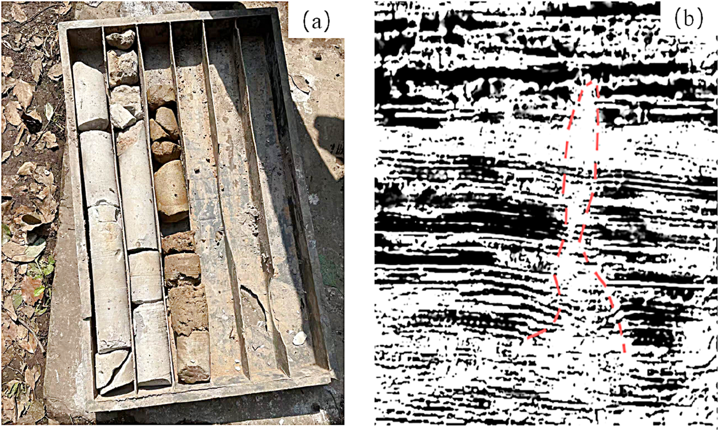
Figure of the study area for KCPs exploration: (a) surface drilling and coring; (b) 3D seismic interpretation.
In the study area, structural development is predominantly monoclinic, oriented northeast and trending northwest, with dip angles ranging from 2° to 10°. The gentle folds and small positive faults are also developed in the minefield. Specifically, 7 short-axis synclines and anticlines are present, with both wings exhibiting inclination angles less than 12°. Most geological conditions in the No. 3 and No. 15 coal seams are exposed, enabling precise fold mapping based on the bottom plate contour lines. In terms of fault development, 14 faults have been identified through surface drilling, 3-D seismic exploration and underground mining (Figure 3), with displacements varying from 1.5 m to 22 m. Faults with approximately 22 m of displacement have been exposed both on the surface and underground. Additionally, during No. 3 coal seam mining, 10 small positive faults were identified in the underground roadway, and 3 faults with displacements between 5 m and 10 m were detected through physical exploration.
FIGURE 3
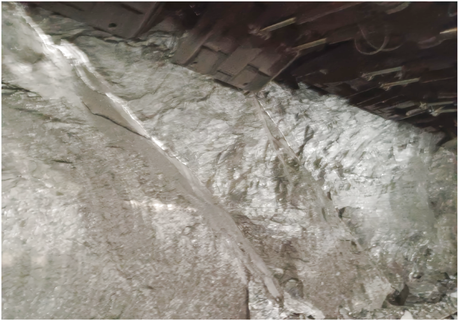
Figure of minor faults exposed by underground mining.
3 Methods
3.1 Overview
In this study, we employed the Moran’s index to identify hotspot distributions of KCPs in the coal mine, aiming to construct a systematic model for their distribution. As shown in Figure 4, before pinpointing these hotspots, it is essential to quantitatively characterize the KCPs within the study area. After identifying the hotspots of KCPs, relevant geological structures such as faults and folds are also discussed to geologically analyze the formation of these special KCPs. The data processing associated with this study is detailed in the subsequent chapters.
FIGURE 4
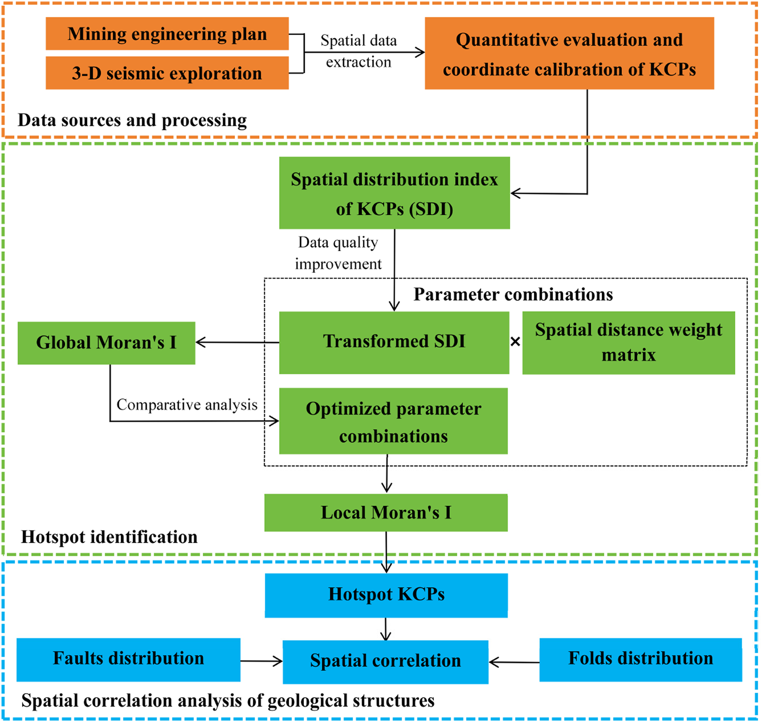
The working steps of the methodology.
3.2 Morphological characteristics of KCP
The spatial morphology of the KCP is one of the most important characteristics, which includes three main types: general morphology characteristics, lateral and vertical development characteristics. Since the general morphology of KCP in the study area is often cone-shaped, the latter two developmental characteristics were analysed.
As shown in Figure 5, lateral characteristics are the characteristics of the plane formed by the intersection of the KCP with the ground level in terms of size and shape. It typically includes a long axis (LA), short axis (SA), and shape description as well as perimeter (P) and area (A). It is worth noting that in this paper, we proposed the calculation of the circularity index (CI), which can be used to transform the non-quantitative shape description into the quantitative characteristic. The transformation is shown in Equation 1:where CI is in the range of [0,1], and when CI is equal to 1, KCP is circle.
FIGURE 5
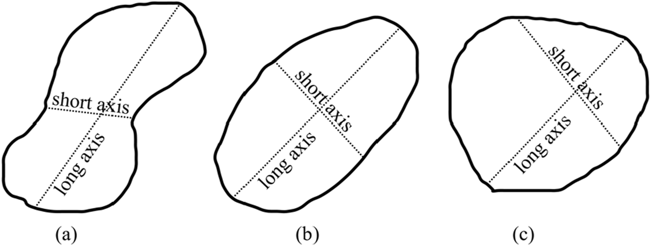
Figure of lateral development characteristics of KCP. (a) Near elliptical shape, (b) Elliptical shape, (c) Nwear circular shape.
The vertical developmental characteristics are characteristics of the plane formed by the intersection of the KCP with the plumb line in terms of size and shape. As shown in Figure 6, it mainly includes the collapse angle (CA), which can be calculated according to Equation 2.where CA is in the range of [0°,90°], , are the equivalent circular radius of the same KCP exposed in the upper and lower coal seams, respectively, and is the elevation difference at the center of the KCP on the contour lines of the upper and lower coal seams floor.
FIGURE 6
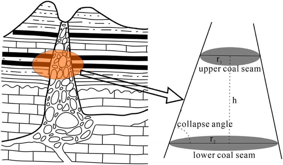
Figure of vertical development characteristics of KCP.
3.3 Calculation of the spatial distribution index
Quantifying the distribution of KCPs in the study area is the basis for hotspot identification. As previously noted, the KCP mainly consists of six main morphological characteristics (Figure 7, stage I): the collapse angle (CA), long axis (LA), short axis (SA), perimeter(P), area(A), and circularity index (CI) obtained from the exposure, respectively.
FIGURE 7
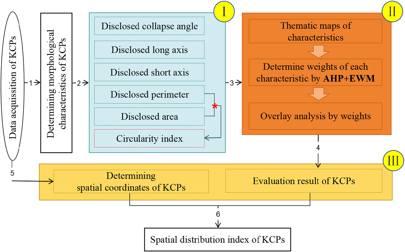
Figure of calculating the spatial distribution index of KCPs.
By integrating the subjective analysis of AHP with the objective weights of EWM (Hu et al., 2019), we constructed a quantitative evaluation method for the morphological characteristics of KCPs (Figure 7, stage II). As shown in Equation 3, assuming that the weights of morphological characteristics obtained using AHP and EWM are denoted by and , respectively, these weights are combined using a coefficient to form a unified weight matrix . Then the quantitative evaluation results of KCPs can be calculated by weighting the morphological characteristics, as in Equation 4.where , and are all 6-by-1 matrix. Assuming .
Finally, to obtain the spatial distribution index of KCPs, the spatial center coordinates of each KCP were calculated in the data acquisition step by using both the mining engineering plan and the 3-D seismic exploration data.
The coordinates were then used to spatially calibrate the evaluation results, thereby deriving the spatial distribution index of the KCPs (Figure 7, stage III). Specifically, a spatial database was constructed in GIS software using the spatial coordinates obtained from the aforementioned 3D seismic interpretation. The calculated attribute data, such as the morphological characteristics of the KCPs, were then assigned corresponding coordinates. This calibration ensures that each SDI (Spatial Distribution Index) value is accurately georeferenced, thereby facilitating spatial analysis within the GIS software.
3.4 Spatial hotspots identification and classification of KCPs
Hotspot extraction theory is used to identify regions with significantly high or low values in spatial attributes (Chang et al., 2023). In this paper, we implement spatial hotspot identification of KCPs by calculating the Moran’s index of sample points, which consists of two parts: the global Moran’s index ()and the local Moran’s index (Gedamu et al., 2024; Tsui et al., 2022).
Firstly, the quantifies the overall spatial autocorrelation within a study area, allowing researchers assess whether significant spatial clustering exists, such as the aggregation trends of high-value hotspots or low-value coldspots. To identify specific hotspots, we first evaluated the spatial aggregation degree of KCPs across the entire well field by applying Equations 5, 6 (Anselin, 1995).
Secondly, unlike the that evaluates spatial autocorrelation on a broad scale, the local Moran’s index focuses on the local spatial patterns. It is used to identify spatial clusters or outliers within a specific region (Tepanosyan et al., 2019). As show in Figure 8, spatial clusters can be categorized into high-high clusters (where high values are surrounded by other high values) and low-low clusters. In contrast, spatial outliers are values that significantly differ from those in their surrounding area, which include high-low outliers (where a high value is surrounded by low values) and low-high outliers (Wu and Song, 2018; Ye et al., 2018).
FIGURE 8
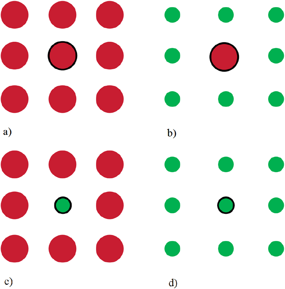
Figure showing the relationship of a location and its neighbourhood: (a,b) hot spots; (c,d) cool spots.
Generally, spatial clusters are areas where high SDI are surrounded by other area with high SDI. In contrast, outliers are locations with high SDI surrounded by samples with normal or low SDI. Thus, after confirming the clustering of SDI values within the well field, the Local Moran’s index is employed to identify spatial clusters and outliers of KCPs by applying Equations 7, 8 (Anselin, 1995).where is the value of the variable SDI at location ; is the average value of SDI with the sample number of , and is a weight which can be defined as the inverse of the distance among locations and . The weight can also be determined using a distance band; samples within a distance band are given the same weight while those outside the distance band are given the weight of 0.
3.5 Data quality improvement
The quantitative evaluation results of KCPs derived from the AHP + EWM method often exhibit poor normality, susceptibility to outliers, and inconsistent data variability across different regions (Wu, 2023). To enhance the accuracy of Moran’s index, especially local Moran’s index, we used the Box-Cox transformation on the SDI defined by Equation 9. This transformation is applied because it can significantly improve the normality, symmetry, and homogeneity of variance in the data (Figure 9) (Osborne, 2010). By aligning the data more closely with a normal distribution, the Box-Cox transformation boosts the reliability of Moran’s index calculations.where is the transformed value, and is the value of original data. For a given data set , the parameter is estimated based on the assumption that the transformed values are normally distributed. When , the transformation becomes the logarithmic transformation.
FIGURE 9
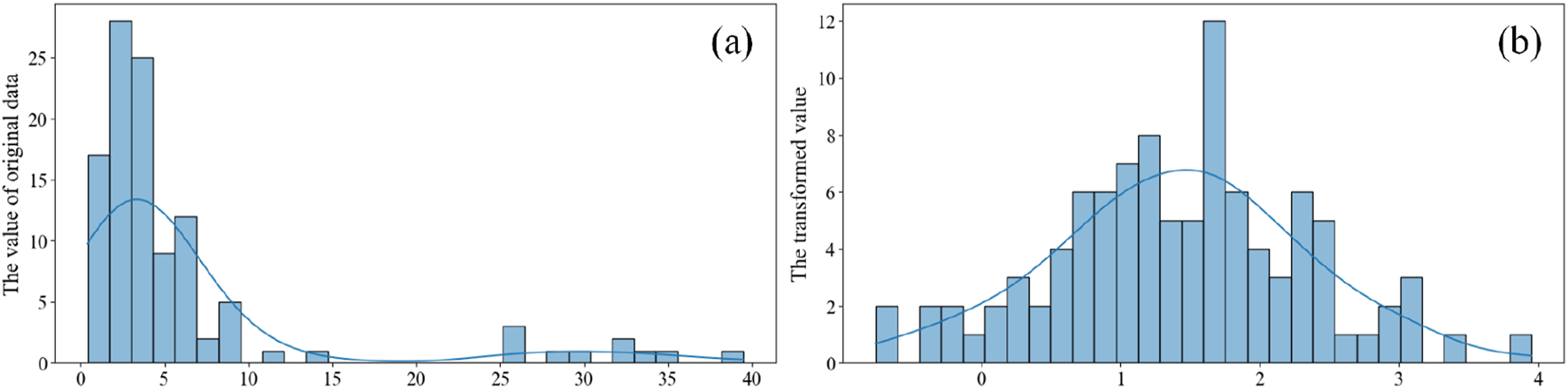
Figure showing changes in data by applying BOX-COX transformation: (a) the value of original data (SDI); (b) the transformed value.
4 Results and discussion
4.1 Spatial distribution index of KCPs
The primary morphological characteristics of the 65 KCPs revealed include both quantitative and non-quantitative characteristics. The non-quantitative characteristics primarily involve shape descriptions of the KCPs. These shape descriptions were quantified into the CI, and we used GIS spatial analysis to visualize the quantitative data (Figure 10). Notably, the collapse angle of the KCPs is consistently around 70°, and thus was not visualized using GIS. Instead, it was incorporated as a parameter in the quantitative evaluation process.
FIGURE 10
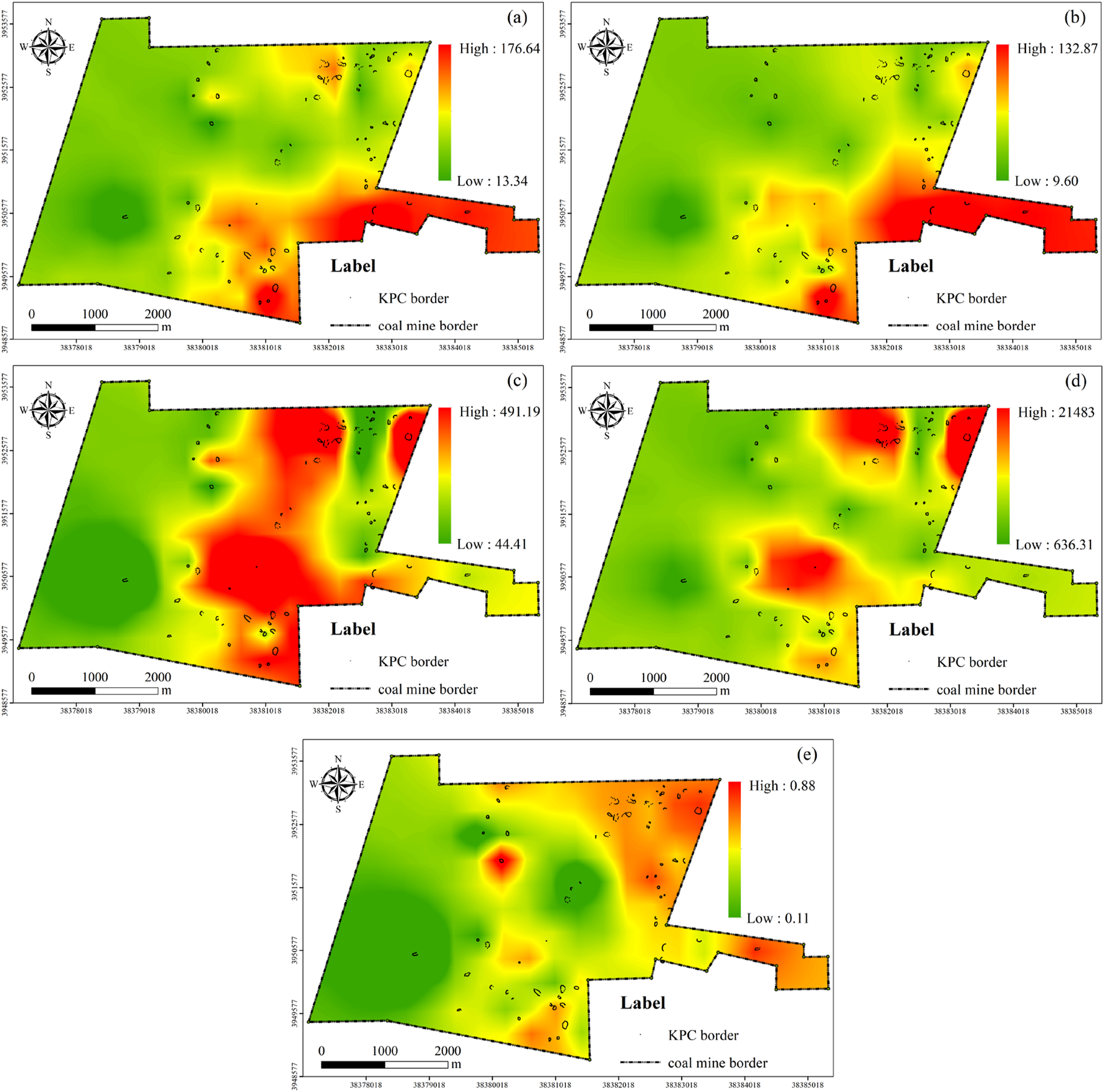
Thematic maps of each morphological characteristic of KCPs: (a) Long axis; (b) Short axis; (c) Perimeter; (d) Srea; (e) Circularity index.
To enhance the reliability of the subjective weighting process in the AHP method, we constructed a pairwise comparison matrix based on expert judgments regarding the relative importance of six morphological characteristics. The constructed pairwise comparison matrix is shown in Table 1. After normalizing the matrix and computing the eigenvector, the resulting weight vector reflects the relative contribution of each characteristic. Furthermore, the consistency of the judgment matrix was evaluated by calculating the Consistency Ratio (CR), defined by Equation 10.where is the consistency index, and is the random index corresponding to the matrix size.
TABLE 1
| Characteristics | LA | SA | P | A | CI | CA |
|---|---|---|---|---|---|---|
| LA | 1 | 1 | 2 | 3 | 1/2 | 5 |
| SA | 1 | 1 | 3 | 3 | 1/2 | 5 |
| P | 1/2 | 1/3 | 1 | 2 | 1/4 | 2 |
| A | 1/3 | 1/3 | 1/2 | 1 | 1/5 | 2 |
| CI | 2 | 2 | 4 | 5 | 1 | 7 |
| CA | 1/5 | 1/5 | 1/2 | 1/2 | 1/7 | 1 |
Single-Level AHP judgment matrix of six morphological characteristics.
The calculated CR value was 0.0098, which is below the acceptable threshold of 0.1, indicating that the pairwise comparisons are consistent and the judgment matrix is reliable.
In the quantitative evaluation of KCPs in the Wangpo coal mine, the weights for six main morphological characteristics are presented in Table 2. It's worth noting that the weights of collapse angle calculated are all zeros, since that in the study area are all around 70°. After calculating the weights using the AHP and EWM methods, these weights were combined using a weight with . The final weights are thus: .
TABLE 2
| Morphological characteristics | CA () | LA () | SA () | P () | A () | CI () |
|---|---|---|---|---|---|---|
| 0.04 | 0.20 | 0.22 | 0.10 | 0.07 | 0.37 | |
| 0.00 | 0.19 | 0.20 | 0.10 | 0.48 | 0.03 | |
| 0.02 | 0.19 | 0.21 | 0.10 | 0.27 | 0.20 |
The weight of the 6 main morphological characteristics by applying AHP, EWM and AHP + EWM.
The layers of every main morphological characteristics that store information are compounded into one upper layer including all information of relevant characteristic. In addition to this, the obtained spatial coordinates were utilized to calibrate each quantitative characteristics. Then, the SDI is calculated as Equation 11, and Table 3 shows the SDI for the 65 sample points in the study area.where is the spatial distribution index of the KCPs, is the weight of morphological characteristics, is a function about single-characteristics value; , and is the geographic coordinate and the 3-D seismic exploration, and is the number of characteristics.
TABLE 3
| Id | Value | Id | Value | Id | Value | Id | Value | Id | Value |
|---|---|---|---|---|---|---|---|---|---|
| X1 | 0.1236 | X14 | 0.0506 | X27 | 0.0715 | X40 | 0.1371 | X53 | 0.1274 |
| X2 | 0.1173 | X15 | 0.0640 | X28 | 0.0804 | X41 | 0.0513 | X54 | 0.0430 |
| X3 | 0.1831 | X16 | 0.0849 | X29 | 0.0639 | X42 | 0.1014 | X55 | 0.0660 |
| X4 | 0.1477 | X17 | 0.2566 | X30 | 0.1394 | X43 | 0.0546 | X56 | 0.0816 |
| X5 | 0.0856 | X18 | 0.0427 | X31 | 0.1072 | X44 | 0.0647 | X57 | 0.0652 |
| X6 | 0.1045 | X19 | 0.1136 | X32 | 0.1973 | X45 | 0.0970 | X58 | 0.1757 |
| X7 | 0.0863 | X20 | 0.079 | X33 | 0.1895 | X46 | 0.0555 | X59 | 0.0980 |
| X8 | 0.0524 | X21 | 0.0835 | X34 | 0.0951 | X47 | 0.0694 | X60 | 0.0477 |
| X9 | 0.0462 | X22 | 0.0547 | X35 | 0.109 | X48 | 0.0687 | X61 | 0.0789 |
| X10 | 0.1337 | X23 | 0.2099 | X36 | 0.0713 | X49 | 0.0414 | X62 | 0.0420 |
| X11 | 0.3207 | X24 | 0.1113 | X37 | 0.0689 | X50 | 0.0675 | X63 | 0.0731 |
| X12 | 0.0757 | X25 | 0.1066 | X38 | 0.1606 | X51 | 0.1186 | X64 | 0.0640 |
| X13 | 0.0581 | X26 | 0.1101 | X39 | 0.1082 | X52 | 0.1337 | X65 | 0.0765 |
The SDI values for 65 KCPs.
As shown in Figure 11, spatial interpolation of the SDI for the 65 calibrated KCPs was conducted using a bilinear interpolation algorithm. This process achieved interpolation accuracies of 100 m, 100 m, and 1 m along the , and axes, allowing for the derivation of SDI values across the whole coal mine.
FIGURE 11

Figure of whole mine spatial SDI interpolation (sliced at 600 m intervals in x, y-axes).
4.2 Effects of different parameters on hotspots identification
In calculating Moran’s index, selecting both attribute values and the spatial distance weight matrix is crucial. Although Moran’s index does not require strict adherence to normality, attribute values approximating a normal distribution generally improve the reliability of significance testing. Therefore, we evaluated the impact of raw data (Table 2) versus BOX-COX transformed data (Table 4) on . As shown in Figure 12, the normal distribution of the SDI values after transformation by the Box-Cox algorithm is greatly improve.
TABLE 4
| Id | Value | Id | Value | Id | Value | Id | Value | Id | Value |
|---|---|---|---|---|---|---|---|---|---|
| X1 | −7.0914 | X14 | −18.7608 | X27 | −12.9944 | X40 | −6.294 | X53 | −6.8488 |
| X2 | −7.5286 | X15 | −14.6251 | X28 | −11.4447 | X41 | −18.4915 | X54 | −22.2377 |
| X3 | −4.4611 | X16 | −10.7826 | X29 | −14.6502 | X42 | −8.8653 | X55 | −14.1514 |
| X4 | −5.7706 | X17 | −2.8966 | X30 | −6.1714 | X43 | −17.3198 | X56 | −11.2597 |
| X5 | −10.684 | X18 | −22.4442 | X31 | −8.3255 | X44 | −14.4602 | X57 | −14.3286 |
| X6 | −8.5714 | X19 | −7.7995 | X32 | −4.0679 | X45 | −9.3129 | X58 | −4.6909 |
| X7 | −10.5815 | X20 | −11.6598 | X33 | −4.2778 | X46 | −17.0026 | X59 | −9.201 |
| X8 | −18.0992 | X21 | −10.9756 | X34 | −9.5132 | X47 | −13.4038 | X60 | −19.943 |
| X9 | −20.6516 | X22 | −17.2701 | X35 | −8.1785 | X48 | −13.5483 | X61 | −11.679 |
| X10 | −6.4815 | X23 | −7.4301 | X36 | −13.0259 | X49 | −23.1536 | X62 | −22.8042 |
| X11 | −2.1179 | X24 | −7.9852 | X37 | −13.504 | X50 | −13.8107 | X63 | −12.6888 |
| X12 | −12.2021 | X25 | −8.3819 | X38 | −5.2283 | X51 | −7.4301 | X64 | −14.6346 |
| X13 | −16.2236 | X26 | −8.0836 | X39 | −8.2438 | X52 | −6.4813 | X65 | −12.0795 |
The SDI values for 65 KCPs after BOX-COX transformation when .
FIGURE 12
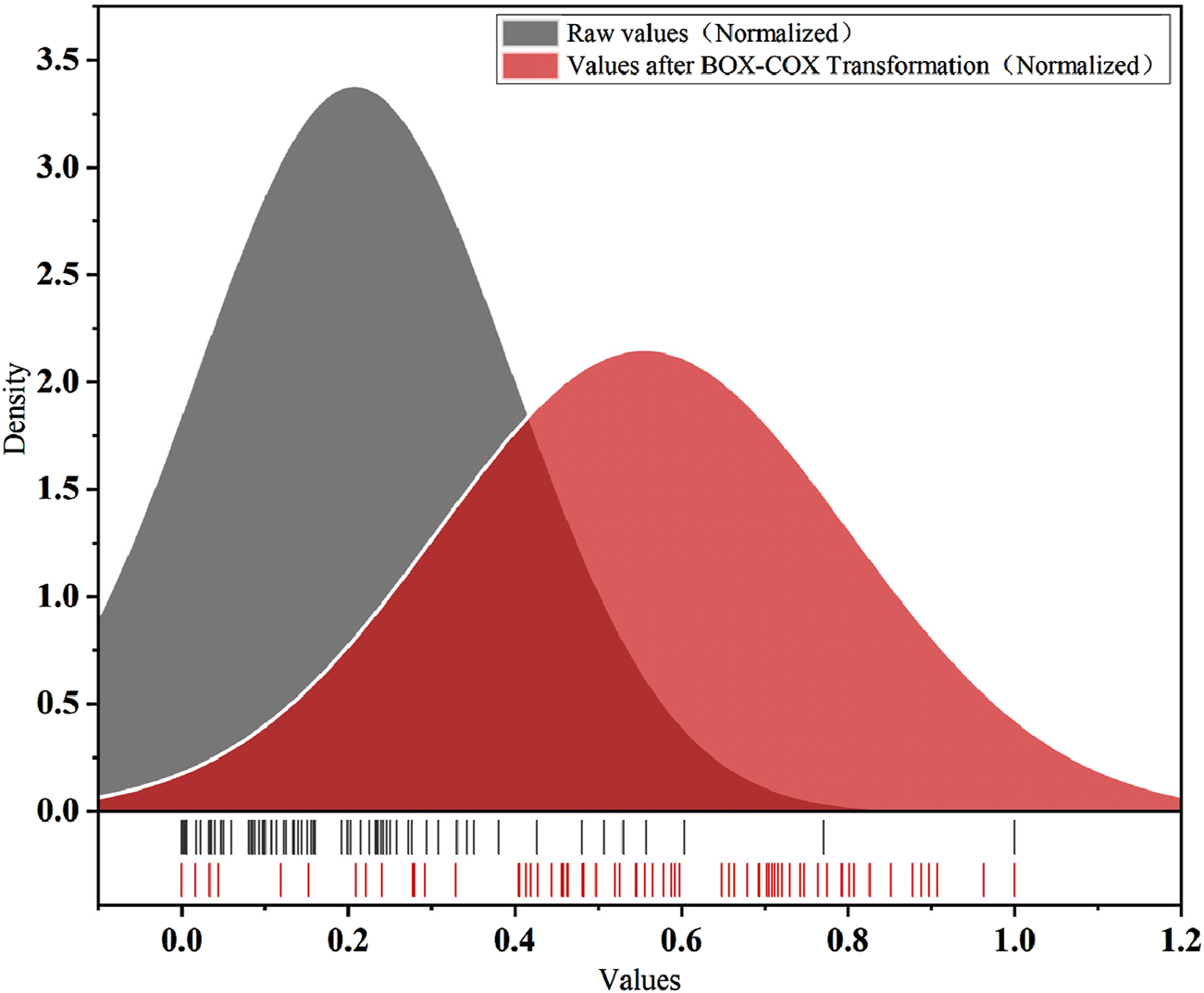
Sketch map of normal distributability of SDI values before and after quality improvement.
Furthermore, an appropriate spatial weight matrix is essential for accurately representing the spatial relationships between sample points. For this purpose, distance bands (d = 150 m, d = 300 m, d = 500 m) were employed to construct the spatial weight matrix based on both the geological characteristics of the study area. Specifically, the 150 m band corresponds to the minimum spacing between closely distributed KCPs, particularly those formed along minor folds and small-scale fault systems identified in underground roadways. The 300 m distance aligns well with the average fault spacing and influence radius of major structural zones in the Wangpo coal mine. This distance also approximates the geological control radius for hydrogeological interaction between faults and collapse features in similar North China coalfields. The 500 m band was included as a broader regional control scale, encompassing the structural influence of major fold axes and long-displacement faults.
As shown in Figure 13, we tested 6 experimental scenarios by examining all possible combinations of these two parameters to ensure comprehensive analysis.
FIGURE 13
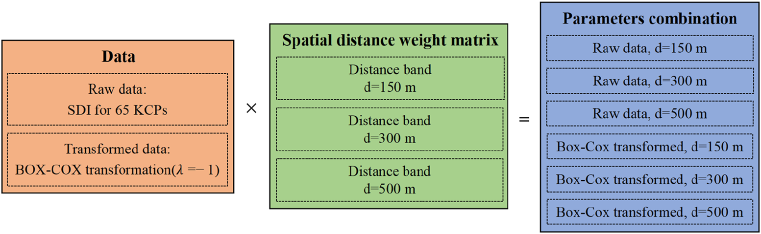
Sketch map of the Cartesian product of data transformations and spatial distance weight matrix combinations.
Except for the third combination (raw data, d = 500 m), all other combinations yielded positive , indicating a positive spatial autocorrelation of KCPs within the study area (Table 5). Furthermore, the use of Box-Cox transformed SDI enhanced the calculation effect of compared to raw data, demonstrating that the transformed SDI values were more effective. Additionally, a more optimal of 0.1110 was achieved using a distance band of d = 300 m in the analysis.
TABLE 5
| Combination number | Data treatment | Std. Dev | p-value | 95% Confidence Interval | |
|---|---|---|---|---|---|
| 1 | Raw data, d = 150 m | 0.0699 | 0.0271 | 0.008 | (0.0178, 0.1220) |
| 2 | Raw data, d = 300 m | 0.0365 | 0.0234 | 0.032 | (-0.0093, 0.0823) |
| 3 | Raw data, d = 500 m | −0.0397 | 0.0258 | 0.041 | (-0.0903, 0.0109) |
| 4 | Box-Cox transformed, d = 150 m | 0.0757 | 0.0267 | 0.017 | (0.0233, 0.1281) |
| 5 | Box-Cox transformed, d = 300 m | 0.1110 | 0.0314 | 0.025 | (0.0492, 0.1728) |
| 6 | Box-Cox transformed, d = 500 m | 0.0273 | 0.0226 | 0.026 | (-0.0169, 0.0715) |
of the study area under different parameter combinations.
Among the six tested combinations, the fifth combination (Box-Cox transformed, d = 300 m) was selected for the calculation of the local Moran’s index. This configuration yielded the highest global Moran’s I value (0.1110), with a statistically significant p-value (0.025) and a 95% confidence interval excluding zero. It also aligns well with the average fault spacing in the study area, ensuring geological relevance. Moreover, the Box-Cox transformation improved data normality, enhancing the reliability of spatial statistical results. This approach was chosen to effectively capture the spatial distribution and clustering patterns of KCPs within the study area. The results of this analysis were visualized (Figure 14) to delineate and map the spatial aggregation hotspots of KCPs.
FIGURE 14
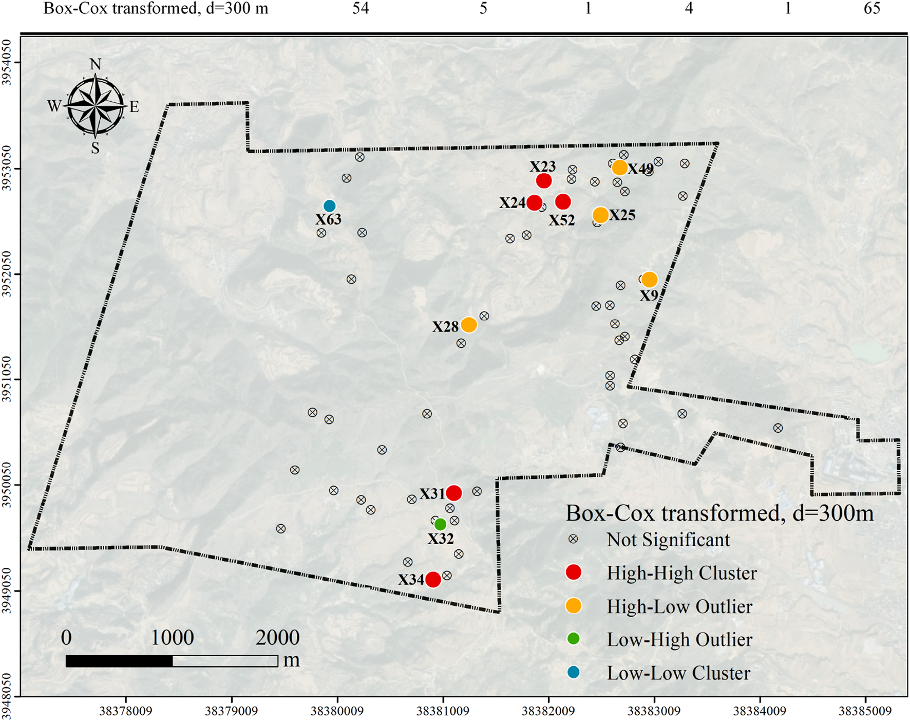
Statistics of localized Moran’I results of SDI and Sketch figure of hotspots distribution in the study area.
Based on the statistical results and spatial analysis, the study area reveals the following four distinct spatial patterns:
• High-High Clusters: These clusters represent regions with significant concentrations of high SDI. The identified High-High clusters are located at KCP X23, X24, X31, X32, X34, and X52. These clusters indicate areas where high SDI are spatially aggregated and substantially exceed the values found in adjacent regions. Such patterns usually signify a more extensive development of KCPs in that area of the mine.
• High-Low Outliers: The identified High-Low outliers X9, X25, X28, and X49 are characterized by high SDI surrounded by areas with lower SDI. These outliers stand out as exceptional high-value points in an otherwise lower-value context, suggesting the possibility of more highly developed KCPs in these regions.
• Low-Low Cluster: The Low-Low cluster identified at X63 represents a spatially concentrated area with low SDI. This cluster highlights regions where low values are aggregated, indicating a significant concentration of areas with less extensive KCP development compared to surrounding regions.
• Low-High Outlier: The Low-High outlier identified at X32. This pattern highlights a point of deviation where low SDI are situated within an otherwise high SDI area, which suggests that some of the KCPs in the region were disturbed by geological factors and thus ceased to develop.
4.3 Spatial correlation analysis of geological structure distribution and different KCPs hotspot
According to the geological report, the controlling factors of the KCPs mainly include hydrodynamics, subordinate dissolution rocks and geological structure within the Wangpo coal mine. Further, in order to analyse the geological development law of the four types of KCPs mentioned above, we plotted the geological structure including faults and folds with the obtained special KCPs on the geological map with contour lines. From a large-scale perspective, most of the KCPs obtained are located near geological structure development zones, opening up the possibility of local analyses.
As shown in Figure 15, the most obvious is the high-high cluster type of KCPs, which mainly includes X23, X24, X52, and X31, all located at the intersections of folds and faults. The results are consistent with previous studies conducted by (Tîrlă and Vijulie, 2013; Li et al., 2022), which indicates that the geological conditions at the junctions of faults and folds have strong structural control for the development of KCPs, and suggesting that these special areas have a higher density of KCPs and a correspondingly greater risk.
FIGURE 15

Schematic diagram of special KCPs and geological structure.
Secondly, compared to the theory that large-scale KCPs is associated with faults proposed by (Qi et al., 2014), this study presents high-low outlier and low-low cluster type KCPs, including X25, X28 and X63, are also located within the development of folds. The low-high outlier type KCPs were not found to be associated with geological structure distribution.
In addition, it is worth noting that low-low cluster type (X63) and high-low outlier type (X28) KCPs occur in both the Yangshancun folds, and it can be assumed that a certain size of KCPs are distributed near the Yangshancun folds.
5 Conclusion
To classify distribution patterns of KCPs and identify high-risk KCPs, this study proposed a method on hotspot identification based on the Moran’s index for the spatial distribution of KCPs. The study involves the quantification of the spatial distribution of KCPs, calculation of the Moran’s index for SDI, and analysis of hotspot KCPs’ distribution patterns. The main conclusions are as follows:
1 Spatial distribution index (SDI) construction: The AHP and EWM were used to determine the weight of KCPs’ morphology characteristics. Through overlay analysis and spatial coordinate calibration, the SDI was obtained. This index effectively quantifies KCPs within the mining area, providing a data foundation for hotspot identification.
2 Optimal parameters for Moran’s index calculation: In the Wangpo coal mine, the SDI transformed by the BOX-COX algorithm and distance band of d = 300 m are suitable for calculating the Moran’s index. With these parameters, four special types of KCPs were identified: high-high cluster, low-low cluster, low-high outlier, and high-low outlier. Each type of KCP has its unique developmental characteristics.
3 Spatial distribution analysis of special KCPs: The spatial distribution patterns of the four special KCP types were analysed in relation to faults and folds. Particularly, the high-high cluster type of KCPs aligns with the geological data of Wangpo coal mine, primarily found at the intersections of faults and folds.
4 Limitations and Future Work: The method is limited by spatial resolution and simplified structural assumptions. Future research may integrate machine learning for automated classification, apply the approach to other geohazards (e.g., sinkholes, landslides), and extend it to time-series data for dynamic monitoring and early warning.
Statements
Data availability statement
The original contributions presented in the study are included in the article/Supplementary Material, further inquiries can be directed to the corresponding author.
Author contributions
JY: Software, Writing – original draft, Resources, Visualization, Investigation, Writing – review and editing, Project administration, Validation, Formal Analysis, Methodology, Supervision, Data curation, Conceptualization. ZL: Writing – review and editing, Funding acquisition. HY: Funding acquisition, Writing – review and editing, Investigation. LA: Investigation, Writing – review and editing. WL: Writing – review and editing. TW: Visualization, Writing – review and editing. QX: Writing – review and editing, Data curation. CL: Software, Writing – review and editing.
Funding
The author(s) declare that financial support was received for the research and/or publication of this article. Supported by the National Natural Science Foundation of China (42374176); Key Research and Development Program of Shaanxi Province (2025CY-YBXM-485); Science and Technology Innovation Fund of Xi’an CCTEG Transparent Geology Technology Co. Ltd. (2024-TM-ZX001).
Conflict of interest
Authors JY, ZL, HY, LA, TW, QX, and CL were employed by Xi'an Research Institute Co. Ltd., China Coal Technology and Engineering Group Corp.
Authors JY, ZL, HY, LA, QX, and CL were employed by Xi'an CCTEG Transparent Geology Technology Co. Ltd.
The remaining author declares that the research was conducted in the absence of any commercial or financial relationships that could be construed as a potential conflict of interest.
The authors declare that this study received funding from Xi'an CCTEG Transparent Geology Technology Co. Ltd. The funder had the following involvement in the study: providing support in project design and data acquisition, as well as technical guidance related to the spatial quantitative analysis of Karst Collapse Pillars.
Generative AI statement
The author(s) declare that no Generative AI was used in the creation of this manuscript.
Any alternative text (alt text) provided alongside figures in this article has been generated by Frontiers with the support of artificial intelligence and reasonable efforts have been made to ensure accuracy, including review by the authors wherever possible. If you identify any issues, please contact us.
Publisher’s note
All claims expressed in this article are solely those of the authors and do not necessarily represent those of their affiliated organizations, or those of the publisher, the editors and the reviewers. Any product that may be evaluated in this article, or claim that may be made by its manufacturer, is not guaranteed or endorsed by the publisher.
Supplementary material
The Supplementary Material for this article can be found online at: https://www.frontiersin.org/articles/10.3389/feart.2025.1593432/full#supplementary-material
References
1
Andriani G. F. Loiotine L. (2020). Multidisciplinary approach for assessment of the factors affecting geohazard in karst valley: the case study of Gravina di Petruscio (Apulia, South Italy). Environ. Earth Sci.79 (19), 458. 10.1007/s12665-020-09212-y
2
Anselin L. (1995). Local indicators of spatial association—LISA. Geogr. Anal.27 (2), 93–115. 10.1111/j.1538-4632.1995.tb00338.x
3
Bai H. Ma D. Chen Z. (2013). Mechanical behavior of groundwater seepage in karst collapse pillars. Eng. Geol.164, 101–106. 10.1016/j.enggeo.2013.07.003
4
Chalikakis K. Plagnes V. Guerin R. Valois R. Bosch F. P. (2011). Contribution of geophysical methods to karst-system exploration: an overview. Hydrogeology J.19 (6), 1169–1180. 10.1007/s10040-011-0746-x
5
Chang S. Zhao J. Jia M. Mao D. Wang Z. Hou B. (2023). Land use change and hotspot identification in harbin–changchun urban agglomeration in China from 1990 to 2020. ISPRS Int. J. Geoinf.12 (2), 80. 10.3390/ijgi12020080
6
Cooley T. (2002). Geological and geotechnical context of cover collapse and subsidence in mid-continent US clay-mantled karst. Environ. Geol.42 (5), 469–475. 10.1007/s00254-001-0507-6
7
Gedamu W. T. Plank-Wiedenbeck U. Wodajo B. T. (2024). A spatial autocorrelation analysis of road traffic crash by severity using Moran’s I spatial statistics: a comparative study of Addis Ababa and Berlin cities. Accid. Anal. Prev.200, 107535. 10.1016/j.aap.2024.107535
8
Gui H. Qiu H. Chen Z. Ding P. Zhao H. Li J. (2020). An overview of surface water hazards in China coal mines and disaster-causing mechanism. Arab. J. Geosci.13 (2), 67. 10.1007/s12517-019-5046-0
9
He K. Guo D. Du W. Wang R. (2007). The effects of karst collapse on the environments in north China. Environ. Geol.52, 449–455. 10.1007/s00254-006-0478-8
10
He K. Yu G. Lu Y. (2009). Palaeo-karst collapse pillars in northern China and their damage to the geological environments. Environ. Geol.58, 1029–1040. 10.1007/s00254-008-1583-7
11
Hu Y. Li W. Wang Q. Liu S. Wang Z. (2019). Evaluation of water inrush risk from coal seam floors with an AHP–EWM algorithm and GIS. Environ. Earth Sci.78, 290–15. 10.1007/s12665-019-8301-5
12
Huang Y. Tao C. Liang J. Liao S. Wang Y. Chen D. et al (2021). Geological characteristics of the Qiaoyue Seamount and associated ultramafic-hosted seafloor hydrothermal system (∼52.1° E, Southwest Indian Ridge). Acta Oceanol. Sin.40, 138–146. 10.1007/s13131-021-1832-0
13
Jiang X. Dai J. Zheng Z. Li X. J. Ma X. Zhou W. et al (2025). An overview on karst collapse mechanism in China. Carbonates Evaporites39 (3), 71. 10.1007/s13146-024-00986-x
14
Li C. Yao B. Ma Q. (2018). Numerical simulation study of variable‐mass permeation of the broken rock mass under different cementation degrees. Adv. Civ. Eng.2018 (1), 3592851. 10.1155/2018/3592851
15
Li Y. W. Cui Q. L. Wu Q. Sun J. (2022). Geological risks and countermeasures for mountain tunneling through a large karst cave in Southwest Hubei, China: a case study. Arabian J. Geosciences15 (11), 1083. 10.1007/s12517-022-10331-y
16
Li P. Wu J. Zhou W. LaMoreaux J. W. (2023). Karst collapse and its management[M]/Hazard hydrogeology. Cham: Springer International Publishing, 105–141.
17
Lin W. Li X. Li T. (2025). Multi-source image feature extraction and segmentation techniques for karst collapse monitoring. Front. Earth Sci.13, 1543271. 10.3389/feart.2025.1543271
18
Lu Y. Wu B. He M. Wang L. Huang Z. (2020). Prediction of fracture evolution and groundwater inrush from karst collapse pillars in coal seam floors: a micromechanics‐based stress‐seepage‐damage coupled modeling approach. Geofluids2020 (1), 1–21. 10.1155/2020/8830304
19
Ma D. Wang J. Li Z. (2019). Effect of particle erosion on mining-induced water inrush hazard of karst collapse pillar. Environ. Sci. Pollut. Res.26, 19719–19728. 10.1007/s11356-019-05311-x
20
Osborne J. (2010). Improving your data transformations: applying the Box-Cox transformation. Pract. Assessm. Res. Eval.15 (1), 12. 10.7275/qbpc-gk17
21
Qi J. Zhang B. Zhou H. Marfurt K. (2014). Attribute expression of fault-controlled karst—fort Worth Basin, Texas: a tutorial. Interpretation2 (3), SF91–SF110. 10.1190/int-2013-0188.1
22
Soni A. Monsalve J. J. Bishop R. Ripepi N. Baggett J. G. (2022). Estimating strength of pillars with karst voids in a room-and-pillar limestone mine. Min. Metall. Explor.39 (3), 1073–1086. 10.1007/s42461-022-00594-0
23
Tepanosyan G. Sahakyan L. Zhang C. Saghatelyan A. (2019). The application of Local Moran's I to identify spatial clusters and hot spots of Pb, Mo and Ti in urban soils of Yerevan. Appl. Geochem.104, 116–123. 10.1016/j.apgeochem.2019.03.022
24
Tîrlă L. Vijulie I. (2013). Structural–tectonic controls and geomorphology of the karst corridors in alpine limestone ridges: southern Carpathians, Romania. Geomorphology197, 123–136. 10.1016/j.geomorph.2013.05.003
25
Tsui T. Derumigny A. Peck D. van Timmeren A. Wandl A. (2022). Spatial clustering of waste reuse in a circular economy: a spatial autocorrelation analysis on locations of waste reuse in The Netherlands using global and local Moran’s I. Front. Built Environ.8, 954642. 10.3389/fbuil.2022.954642
26
Wen L. Cheng J. Yang S. Li F. Liu A. Yang Y. (2023). Seismic structure-constrained inversion of CSAMT data for detecting karst caves. Explor. Geophys.54 (1), 55–67. 10.1080/08123985.2022.2065916
27
Wu Y. (2023). “Construction of the China financial pressure index measurement model based under the AHP-EWM-TOPSIS model,” in Proc. SHS web of conferences 01018.
28
Wu H. Song T. (2018). An evaluation of landslide susceptibility using probability statistic modeling and GIS's spatial clustering analysis. Hum. Ecol. Risk Assess.24 (7), 1952–1968. 10.1080/10807039.2018.1435253
29
Xu Z. Sun Y. Gao S. Chen H. Yao M. Li X. (2021). Comprehensive exploration, safety evaluation and grouting of karst collapse columns in the Yangjian coalmine of the Shanxi province, China. Carbonates Evaporites36, 16–12. 10.1007/s13146-021-00675-z
30
Ye W.-F. Ma Z.-Y. Ha X.-Z. Yang H.-C. Weng Z.-X. (2018). Spatiotemporal patterns and spatial clustering characteristics of air quality in China: a city level analysis. Ecol. Indic.91, 523–530. 10.1016/j.ecolind.2018.04.007
31
Zhang B. Liu G. Li Y. Lin Z. (2023). Experimental study on the seepage mutation of natural karst collapse pillar (KCP) fillings over mass outflow. Environ. Sci. Pollut. Res.30 (51), 110995–111007. 10.1007/s11356-023-30230-3
Summary
Keywords
morphological characteristics, geographic information system, coordinate calibration, spatial distribution index, development patterns
Citation
Yan J, Liu Z, Yang H, An L, Li W, Wang T, Xie Q and Liu C (2025) Identifying hotspots and classifying the spatial distribution pattern of karst collapse pillars with Moran’s index in coal mine. Front. Earth Sci. 13:1593432. doi: 10.3389/feart.2025.1593432
Received
14 March 2025
Accepted
05 August 2025
Published
26 August 2025
Volume
13 - 2025
Edited by
Mahdi Hasanipanah, Duy Tan University, Vietnam
Reviewed by
Danial Jahed Armaghani, University of Technology Sydney, Australia
Jinsong Fan, National University of Singapore, Singapore
Updates
Copyright
© 2025 Yan, Liu, Yang, An, Li, Wang, Xie and Liu.
This is an open-access article distributed under the terms of the Creative Commons Attribution License (CC BY). The use, distribution or reproduction in other forums is permitted, provided the original author(s) and the copyright owner(s) are credited and that the original publication in this journal is cited, in accordance with accepted academic practice. No use, distribution or reproduction is permitted which does not comply with these terms.
*Correspondence: Zaibin Liu, liuzaibin@cctegxian.com
Disclaimer
All claims expressed in this article are solely those of the authors and do not necessarily represent those of their affiliated organizations, or those of the publisher, the editors and the reviewers. Any product that may be evaluated in this article or claim that may be made by its manufacturer is not guaranteed or endorsed by the publisher.