Water exchange in the Baltic Sea: a historical view of research approaches from basin scales to submesoscale

Elken, Jüri; Omstedt, Anders

doi:10.3389/feart.2025.1598983

REVIEW article

Front. Earth Sci., 08 July 2025

Sec. Interdisciplinary Climate Studies

Volume 13 - 2025 | https://doi.org/10.3389/feart.2025.1598983

This article is part of the Research TopicNew Challenges for Baltic Sea Earth System ResearchView all 8 articles

Water exchange in the Baltic Sea: a historical view of research approaches from basin scales to submesoscale

Jüri Elken¹*

Anders Omstedt²

¹Department of Marine Systems, Tallinn University of Technology, Tallinn, Estonia
²Department of Marine Sciences, University of Gothenburg, Gothenburg, Sweden

At the beginning of the 20th century, Knudsen illustrated that the mean observed salinity of the Baltic Sea could be realistically estimated, assuming an inflow of saline Kattegat water equals the net freshwater supply, also called the Knudsen theorem. As given in the historical review, several studies have followed the approach of well-mixed boxes, including time variations and a division between different sub-basins in the Baltic Sea. The box concept was later developed into mechanistic models by resolving the vertical structure in each sub-basin and adding processes related to vertical mixing, strait flow dynamics, and exchange with the atmosphere. However, as with the box concept, each sub-basin was assumed to be horizontally homogeneous. Early on, it was clear that the Baltic Sea circulation was highly unsteady, with fronts and eddies at different scales, illustrating a typical marine turbulent flow with energy cascade from basin scale to mesoscale, submesoscale, and microscale, where the energy dissipates. Many observational and modeling studies addressing the three-dimensional structure were developed over the last half-century. The approach of mechanistic models is useful for interpreting large-scale effects of meso- and submesoscale processes and for climate and long-term studies. The submesoscale approaches, including in situ observations, remote sensing, and models resolving the three-dimensional structure, may guide parametrizations of exchange between and within the different sub-basins. Recent submesoscale studies suggest localized eddy-rich regions: Arkona Basin, Gulf of Finland, Irbe Strait, Åland Sea connections, and several coastal areas.

1 Introduction

The Baltic Sea does not have strong currents like the Gulf Stream or Kuroshio that guide essential parts of the ocean water cycle. Instead, the water balance with a surplus of freshwater flow, combined with estuarine salinity gradients, forms mean water exchange flows in the straits connecting the sea with the world ocean or in the straits and deep channels connecting the morphometric subdivisions of the sea. At the same time, sea basins are stratified but horizontally relatively homogeneous, meaning that hydrographic contrasts within the basins are generally smaller than temperature and salinity differences between the basins. Among the water budget components, the inflow of saline water from the North Sea is highly variable. Already in early studies, Kalle (1943) found that a large inflow pulse in 1933/1934 caused an abrupt salinity increase in deep basins like the Eastern Gotland Basin (Figure 1), as noted by Fonselius (1962).

Figure 1

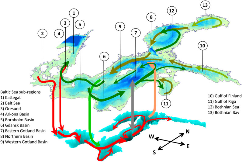
Figure 1. A two-level map of the Baltic Sea, with the surface map given above and permanent halocline sketched below. The arrows represent mean currents in the upper layer (green), the deep layer below the halocline (red), and the flows between the layers. The sub-regions Kattegat, Belt Sea etc are labeled by numbers explained in the legend. Modified from Elken and Matthäus (2008).

Knowledge of governing Baltic Sea water exchange processes has evolved in concert with developments in ocean studies. It is essential for understanding processes in the global and regional Earth System dynamics; using knowledge about the physical system forms the basis for climate and environmental studies. Rather long ago, Fleming and Revelle (1939) summarized three general types of ocean currents: “convection” currents, currents due to wind action, and tidal currents. On smaller scales, turbulent or wave motions appear, but they do not cause any net water transport. Multi-ship observational campaigns were organized in the World Ocean (e.g., International Geophysical Year, 1957–1958) and the Baltic Sea (International Baltic Year, 1969–1970) to further study large-scale physical patterns and processes. A broad spatiotemporal spectrum of oceanic processes became evident by evolving observational techniques, especially for sensor-based fine structure profiling and automatic self-recording mooring stations. Following the traditions in meteorology, a range of these processes obtained the name “variability”. However, systematic divisions of oceanic processes by their temporal and spatial scales, reflecting the energy cascade mechanisms, were synthesized in the 1970s (Monin et al., 1974) after the discovery of oceanic mesoscale eddies (Mode Group, 1978) that have spatial dimensions scaled by Rossby deformation radius R_d.

Specific to the Baltic Sea, hydrographic studies have been coordinated since the 1900s by the International Council for the Exploration of the Sea (ICES) to support fisheries regulations (Leppäranta and Myrberg, 2009). In the 1970s and 1980s, studies that specialized in monitoring the deep basins (Fonselius and Valderrama, 2003) were extended to investigate strait dynamics (Petrén and Walin, 1976), upwelling (Walin, 1972), turbulence (Kullenberg, 1977), and internal waves (Krauss, 1981). Concentrated multi-ship field experiments like BOSEX-1977 (Kullenberg, 1984), PEX-96 (Dybern and Hansen, 1989), and similar individual studies provided an interesting insight into the knowledge of various scale water exchange processes. Because of the limited spatiotemporal coverage, most of the early results of meso-to-small-scale variability studies remained unused in the thematic marine assessments and budget calculations to support environmental management.

The Baltic Sea water cycle was extensively studied in the 20th century, and major research efforts were made in the HELCOM (1986) and BALTEX projects (Raschke et al., 2001). In 1986, the Helsinki Commission (HELCOM) summarized over 10 years of joint efforts in determining the various terms of the Baltic Sea water balance. However, these terms were calculated in isolation, without modeling the Baltic Sea.

In the late 1980s, the Global Energy and Water Experiment (GEWEX) was developed within the World Climate Research Programme (WCRP) framework. The aims were to better understand global, regional, and local processes that exchange energy and water in the climate system. Here, the Baltic Sea served as one of the major sea regions for developing new measuring and modeling efforts. The box model concept served as a conceptual view of the climate problem (Figure 2), and several studies were developed, including observations and models of different complexities. These studies were later analyzed in several reviews (Omstedt et al., 2004; Reckermann et al., 2011; Omstedt et al., 2014; Omstedt and von Storch, 2023). Within the Baltic Earth Assessment Reports (Meier et al., 2023), recent knowledge of Baltic Sea salinity dynamics and related water exchange issues has been overviewed by Lehmann et al. (2022).

Figure 2

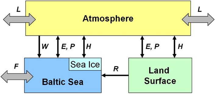
Figure 2. BALTEX I box presents a conceptual view of the Baltic Sea region’s coupled atmosphere, ocean, and land system. The arrows indicate different types of interactions between the boxes (figure courtesy of Marcus Reckermann).

Since the 1980s, different research schools of physical oceanography - the budget approach and meso-to-small scale approach – emerged from observation and modeling technology developments. Initially, these approaches were rather separate, but they have continued to converge in recent years. The Baltic Earth program has stimulated progress in such a convergence. The present review aims at a joint analysis and outline of historical developments of the budget and meso-to-small scale approaches, including submesoscale. In particular, the evolution of research hypotheses and societal needs, combined with enabling technologies, is presented. We also discuss gaps in the knowledge and propose some contemporary research questions.

2 Marine science organization background: need for budgets of water and chemicals

The interest in exploring the sea increased in the 19th century with inspiration from the Challenger expedition (1872–1876), under the command of Charles Wyville Thomson and supported by the British Royal Navy. Expeditions in coastal seas, such as the Baltic Sea, started. In the summer of 1877, Fredrik Laurentz Ekman made temperature and salinity measurements around Sweden, from the Skagerrak to the Bothnian Bay (Ekman and Pettersson, 1893). Similar expeditions were performed by other countries (reported by, e.g., Matthäus, 2006), improving our understanding of the temperature and salinity conditions of the Skagerrak–Baltic Sea system. In the late 19th century, concern arose about the well-being of fish stocks, and scientists from various countries realized that international cooperation was needed, leading to the formation of the International Council for the Exploration of the Sea (ICES) in 1902. The monitoring of oceanographic parameters and fish stock distributions and movements was then implemented, and ICES has since advised fishing regulations to balance the increased fishing pressure.

Water exchange heavily impacts the fate of persistent pollutants like heavy metals, Polychlorinated biphenyls (PCBs), and dioxins, which are deposited into the sea. Pollution of the seas became on the agenda in the 1960s. Jensen et al. (1969) demonstrated that in the Baltic Sea, the levels of chlorinated hydrocarbons are approximately ten times greater than for comparable species in the North Sea area and the Atlantic. In 1969, ICES formed the Working Group on Pollution of the Baltic, which, in the report published in 1974, outlined that “… basic hydrodynamical studies of the mechanisms for exchange and transfer of matter in the Baltic are of prime importance … ” (ICES, 1974). The report listed the study items in physical oceanography for the period beyond 1974 as currents and water exchange, including the exchange and mixing of water masses between the North Sea and the Baltic Sea, exchange with deeper layers in coastal area, mixing in the coastal zone and the exchange with the open sea, mechanisms for horizontal transfer and vertical exchange in the open sea, water motions below the halocline.

Pollution by excess load of nutrients causes eutrophication, resulting in massive algal blooms and oxygen deficiency, controlled mainly by the vertical exchange of nutrients and temporal weakening of lateral deep-water transport of oxygen-rich North Sea waters (Jansson, 1978). The initial goal was to limit the phosphorus and nitrogen loads by 50% in all the sea areas (HELCOM, 1988). These were further developed to determine the nutrient reduction targets based on basin-specific water and nutrient exchange processes (Savchuk and Wulff, 2007) implemented by the Baltic Sea Action Plan (HELCOM, 2013).

The research landscape of the Baltic Sea has many aspects, as presented by Dybern (1980). While applied tasks were defined by ICES and HELCOM, independent research consortia, the Conference of Baltic Oceanographers and Baltic Marine Biologists, had a stimulating role until 1996, when they merged into the Baltic Sea Science Congress. Since the 1990s, projects by the EU and the Nordic Council of Ministers have organized interdisciplinary multinational studies. An important step was the joint Baltic Sea environmental research and development program BONUS, which ran from 2002 to 2022. Among the bottom-up research initiatives, the BALTEX program and its new phase, Baltic Earth, have been active since 1992 (Meier et al., 2023), providing climate change assessments for the Baltic Sea region and many research papers.

3 Mechanistic models of connected sub-basins

Mechanistic models (in their simplest forms, also called box models) start from water and salt conservation laws, including prescribed values on in- and outflows. Early in the 20th century, Knudsen (1900) illustrated that the mean observed salinity of the Baltic Sea could be realistically estimated, assuming an inflow of saline Kattegat water equals the net freshwater supply, also called the Knudsen theorem. Several model studies of water transport have followed, including time variations and a division between the Öresund and the Great Belt (e.g., Burchard et al., 2018; Håkansson, 2022). The BALTEX/Baltic Earth program started from a conceptual view of the water and energy cycles (Figure 2). Significant efforts were undertaken during the program to estimate the different terms in the water balance initially estimated by HELCOM (1986). In the conceptual BALTEX box, the dominant water budget components have been identified as flow of water in and out of the Baltic Sea entrance area (F), together with river runoff (R) and net precipitation (P-E) (Omstedt and Rutgersson, 2000). Net precipitation over the Baltic Sea was further refined by closing the water budget, using new data from ocean modeling, gridded meteorological data, and observed river runoff data (Omstedt et al., 1997; Rutgersson et al., 2002; Meier and Döscher, 2002; Omstedt and Nohr, 2004). In addition, Jacob (2001) used data from the regional atmospheric model and reanalysis data at the atmospheric model’s horizontal boundaries. Extensive field measurements and modeling efforts to study net precipitation were performed by Smedman et al. (2005). Boulahia et al. (2022) conducted a water balance study using satellite data and reanalyzed meteorological data. Using many different approaches and study periods, the net precipitation was estimated to be positive and about 1,500 ± 1,000 m³ s^-1 during the last century. This is one order of magnitude less than the estimated total river runoff, but the same size as the largest Baltic Sea rivers.

Based on the stationary Knudsen theorem, water budgets were developed for the different sub-basins of the Baltic Sea (SNV, 1988; HELCOM, 1993; Figure 3). These concepts formed the basis for long-term environmental studies and for estimating the flow of substances such as nutrients and carbon.

Figure 3

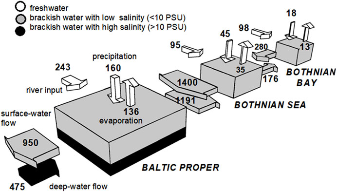
Figure 3. A scheme of stationary water exchange in the Baltic Sea, including the sub-basins Baltic Proper, Bothnian Sea, and Bothnian Bay. The flows in the Baltic Proper also include the Gulf of Finland and the Gulf of Riga. From: The marine environment of Sweden - ecosystems under pressure. Flows in km³ per year. Adopted from SNV (1988).

The box concept was later developed into mechanistic models by adding more basic scientific laws related to vertical mixing, strait flow dynamics, and exchange with the atmosphere. As the first step, Stigebrandt (1983) developed a mechanistic model for the Baltic Sea entrance area. The dynamic in the Baltic Sea entrance area was modeled by only considering the Kattegat and the Belt Sea, both modeled as horizontally homogeneous two-layer sub-models. The model was driven by fresh water supply to the Baltic Sea and sea level variations between the Kattegat and the Baltic Sea, forcing the barotropic and baroclinic exchange flows. The model captured the main features of temporal salinity variations, indicating the validity of applied water exchange formulations. This model was connected with one strait only; studies by Omstedt (1987), Gustafsson (2000a) and Gustafsson (2000b) revealed the importance of adding the Öresund Strait and water temperature when modeling the entrance area.

To include stratification effects within the Baltic Sea sub-basins, Omstedt et al. (1983) and Stigebrandt (1985) developed vertical one-dimensional pycnocline sub-models for temperature and salinity, driven by surface boundary conditions and lateral transports from the neighboring sub-basins. In the stratified water column below the vertically mixed layer, the dense flows from the upstream basin sink to the level of neutral buoyancy and move the overlying layers upward (Stigebrandt, 1985). The mixed layer model covers both the downward entrainment and retreat of the pycnocline. The importance of considering both the temperature and salinity stratification was demonstrated by a study of the cooling of surface water in the Bothnian Bay (Omstedt et al., 1983). Such a model was later used for spin-up simulations, showing that current Baltic Sea conditions could be realistically modeled after the spin-up period, starting from arbitrary initial conditions (Omstedt and Hansson, 2006). Namely, under the forcing by freshwater input and calculated water exchange between the sub-basins, the numerical experiment on the reconstruction of the present-day temperature and salinity regime, starting from the oceanic salinity in the whole Baltic Sea in 1700, reached the contemporary salinities in about 100 years (Figure 4).

Figure 4

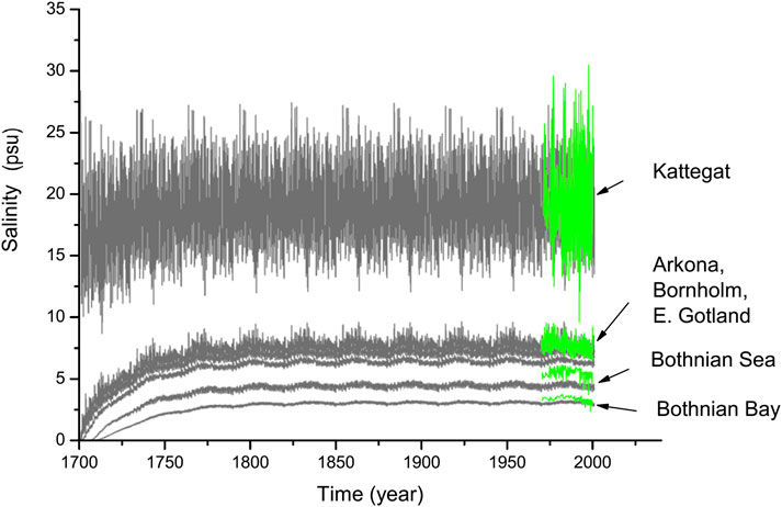
Figure 4. Calculated surface salinity spin-up (grey) from ocean initial conditions using the PROBE-Baltic model of connected basins and observation (green). The forcing data are based on a 30-year period, which was repeated 10 times to reconstruct the 300-year time series. Adopted from Omstedt and Hansson (2006).

Mechanistic models later address the connection of different sub-basins in the Baltic Sea (e.g., Omstedt, 1990; Savchuk et al., 2012), the deep water ventilation in and between the different sub-basins (e.g., Stigebrant, 1987; Kõuts an Omstedt, 1993; Marmefelt, and Omstedt, 1993), sea ice (e.g., Haapala, and Leppäranta, 1996; Leppäranta and Omstedt, 1990; Omstedt, and Nyberg, 1996; Hansson and Omstedt, 2008) and climate studies including long time runs (e.g., Stigebrandt and Gustafsson, 2003; Gustafsson, 2004; Omstedt and Hansson, 2006; Gustafsson and Omstedt, 2009).

The mechanistic models assume that changes in salinity and other model variables along the estuarine gradients are much larger between the basins than within the basins, allowing horizontal integration of variables over these sea basins. Observational evidence for such an assumption stems partly from the long-term monitoring data (e.g., Kõuts and Omstedt, 1993). In the mechanistic models, the exchange flows of water and substances (including salt and heat) between the basins are parameterized by the density and sea level differences. Atmospheric data are also used when appropriate. Generally, the barotropic exchange is calculated using water-level forcing from the Kattegat and river runoff. In straits wider than the local internal Rossby radius, the baroclinic outflows are assumed to be in geostrophic balance (Stigebrandt, 1983; Omstedt, 1990). In narrow straits, such as between the Bothnian Bay and the Bothnian Sea, the baroclinic exchange is considered to be at a maximum flow rate calculated from baroclinic hydraulic control (Omstedt and Axell, 2003).

High-resolution observations, whose data are available from the 1980s, were used to check the horizontally integrated model’s assumptions of a small ratio of within-basin to between-basin salinity variations. Shipborne quasi-synoptic aerial surveys (∼1 day, ∼50 km) on eddy-resolving grids in two regions – the Eastern Gotland Basin and the Bornholm Basin, revealed that large-scale salinity variance between the basins (∼100 km) highly dominates over the mesoscale (∼10 km) spatial variance within one mapping, and the temporal (∼ few days) variability from one mapping to another (Kahru and Aitsam, 1985). Long sections of FerryBox data, measured onboard regularly cruising ships with a resolution of less than 1 km since the beginning of the 1990s (Karlson et al., 2016), have also revealed that surface salinity variations within the basins are much smaller than salinity drops in the frontal areas between the basins, especially between the Bothnian Sea and the Bothnian Bay. Regarding the depth distribution of variability, basin-to-basin salinity differences are larger in the deep layers below the halocline (depth >60 m) than in the layers above.

The classical Knudsen theorem for stationary flows has recently been revisited with high-resolution time-dependent data by Burchard et al. (2018). They used a Total Exchange Flow (TEF) analysis framework, resolved in salinity coordinates instead of depth. By analyzing three-dimensional model results, it was found that ratios of averaged inflowing and outflowing water masses correspond well to the classical estimate based on just a few representative salinity observations. This exemplifies how multitude-scale processes converge to summarize exchange flows.

4 Basin-scale dynamics, fronts and upwelling

The Baltic Sea circulation is highly unsteady, as revealed already from historical observations. Time series of currents are often dominated by 14-h inertial oscillations, first recorded by Gustafsson and Kullenberg (1936). By historical knowledge, there is mostly cyclonic flow in the upper layer (Svansson, 1976; Leppäranta and Myrberg, 2009). The first observational surface current maps were compiled nearly a hundred years ago (e.g., Palmén, 1930), but maps based on numerical models were developed only in the 1970s (Simons, 1978; Kielmann, 1981). Variations of modelled surface currents can be described using dominating patterns (Lehmann and Hinrichsen, 2000; Lehmann et al., 2002; Andrejev et al., 2004; Meier, 2007; Jędrasik et al., 2008; Placke et al., 2018; Maljutenko and Raudsepp, 2019; Barzandeh et al., 2024). In connection with the forcing, geostrophic adjustment tends to make the flow run along the depth contours, as seen in the maps of mean barotropic circulation (Lehmann and Hinrichsen, 2000). The surface currents can be decomposed into ageostrophic currents driven by wind, non-linear interactions, and friction, and geostrophic currents driven by pressure gradients due to sea level and water density. The pattern analysis suggests that cyclonic circulation forming gyres is strongest in December, while in May, the weaker flow may exhibit ageostrophic anticyclonic shears in the coastal regions (Barzandeh et al., 2024). Large-scale currents, including fronts and upwelling, are superimposed by meso- and submesoscale eddies and wave processes like inertial, internal, Poincaré, Kelvin, coastal trapped, and topographic waves (Chapters 5 and 6).

Deep-water flows below the halocline, located in the Baltic Proper at about 60 m depth, generally follow the right-hand slopes of deep sub-basins on its way from the Danish Straits (from Kattegat to Belt Sea and Öresund) to the Western Gotland Basin (Figure 1). Deep layers undergo large variations in flow, salinity and oxygen due to sporadically occurring large inflow pulses of saline water from the North Sea (Matthäus and Franck, 1992; Mohrholz, 2018), termed Major Baltic Inflow (MBI). Figure 5 gives an example of deep water spreading from the Bornholm Basin through the Stolpe Channel to the Eastern Gotland Basin after the November 2002 MBI, using numerical experiments with a tracer (Meier, 2007). There is complicated meso-to-small scale variability of deep water exchange in constrictions like the Bornholm Strait (Petrén and Walin, 1976; Bulczak et al., 2016), Stolpe Channel (Piechura and Beszczynska-Möller, 2004; Zhurbas et al., 2012), and the Farö Channel between the Eastern Gotland Basin and the Northern Basin (Liblik et al., 2022). In the Irbe Strait (Lilover et al., 1998) and the Southern Quark Strait (Muchowski et al., 2023), the deep water inflowing and sinking to the Gulf of Riga and the Bothnian Sea is formed from the surface waters of the Baltic Proper, which have a higher salinity than the waters of these basins. Within the high variability, a significant part of the bulk deep water exchange may be divided into the two components: slowly varying (nearly constant within several months) water exchange (in some cases comparable to the values found from the Knudsen budget) and the fluctuating wind-dependent component. The latter forms the compensation flow to the surface Ekman transport (Krauss and Brügge, 1991), which can be found as a site-specific projection of the wind stress over a larger area to a direction that depends on the location of the transect relative to the basin geometry (Elken et al., 2003; Zhurbas and Väli, 2022). Flows in the straits have often transverse secondary Ekman circulation (Umlauf and Arneborg, 2009; Zhurbas et al., 2012).

Figure 5

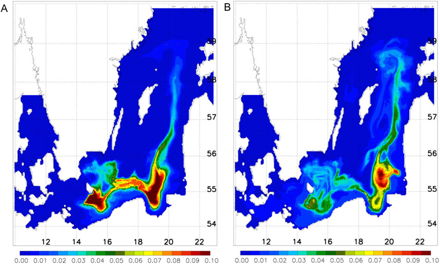
Figure 5. Monthly mean tracer concentration after the Major Baltic Inflow of the North Sea water in November 2002, evolved to January 2003 (A) and March 2003 (B). The results were taken from an experiment when the tracer was initialized in the deep layers of the Bornholm Basin. Adopted from Meier (2007).

Fronts as high-gradient zones are formed when flows between the larger water masses converge, enhancing the horizontal gradients due to frontogenesis (Simpson, 1981; McWilliams, 2021). Such converging flows are often in geostrophic balance according to the Margules’ formula. The width of the frontal current jet is usually smaller than the Rossby deformation radius, but its length may extend to the dimensions of the basins. The frontal zones perform excursions due to meandering and wind drift. The variations within the estuarine salinity gradient are the strongest in the Danish Straits, where salinity drops from about 30 to 8–10 psu (Voss et al., 2011; Lehmann et al., 2022). (We adopted the practical salinity unit psu from historical data and/or figures; for reference, 10 psu corresponds to the absolute salinity of about 10.87 g kg^-1). To the east of these straits, constrictions in the sea topography guide circulation and mixing (Figure 1) that affect the mean surface salinity distribution (Figure 6A). Outside the North Sea-Baltic Sea transition area, permanent forth-and-back migrating fronts are the Quark Front between the Bothnian Sea and Bothnian Bay (salinity drop between the areas from 1 to 3 psu, Green et al., 2006), the Irbe Strait Front between the Eastern Gotland Basin and the Gulf of Riga (salinity drop about 2 psu, Lilover et al., 1998), and the North Baltic Proper Frontal area between the freshened waters of the Gulf of Finland and Bothnian Sea and the saltier waters of the Baltic Proper (Pavelson et al., 1997). Because the positions of fronts vary, the frontal zones are characterized by a higher temporal variance of salinity than the intra-basin areas (Figure 6B; Suursaar et al., 2021).

Figure 6

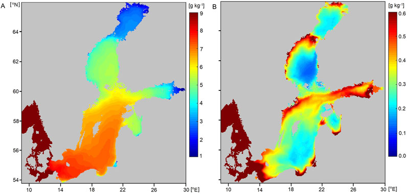
Figure 6. Long-term annual mean salinity (A) and its temporal standard deviation (B) for the period 1993–2019, based on the CMEMS daily reanalysis data (www.copernicus.eu/en/access-data/copernicus-services-catalogue/baltic-sea-physics-reanalysis). Color scales were adjusted for the areas east of the Arkona Basin. Instead of historical salinity unit psu, the absolute salinity g kg^-1 is used as in the model data. From Suursaar et al. (2021).

Fronts also appear in the temperature fields (Kahru et al., 1995; Demchenko et al., 2011; Chrysagi et al., 2021). Most prominent temperature gradients occur in the upwelling fronts, as first outlined by Gidhagen (1987). Part of the thermal fronts reflect the temperature-salinity properties of different water masses formed in the large basins and gulfs and the river influence areas. For thermal fronts, frontogenesis is also guided by differential heating and cooling over variable depth and saline stratification and differential convection when the temperature is close to the value of maximum density.

Upwelling occurs when wind-induced Ekman transport drifts surface waters away from the coast, and deeper waters reach the surface (Lehmann and Myrberg, 2008). Such wind situations are frequently found on the Swedish south and east coasts, the Swedish coast of Bothnian Bay, the southern tip of Gotland, and the Finnish coast of the Gulf of Finland (Lehmann et al., 2012). Upwelling also occurs off the Estonian coast and the Baltic east coast, the Polish coast, and the west coast of Rügen. In the Gulf of Finland, the upwelling waters may cover up to 38% of the gulf’s surface area, while the filaments may cover up to 5% (Uiboupin and Laanemets, 2009). The duration of the upwelling depends on the duration of favorable winds; relaxation after the winds become unfavorable may take several days. Recent knowledge of upwelling in the Baltic Sea has been summarized by Lehmann et al. (2022).

A 2-week upwelling event was observed in August 2006 along the Estonian coast during easterly to southeasterly winds. It was extensively studied using in situ observations (Lips et al., 2009) and modeling combined with remote sensing (Laanemets et al., 2011). Consecutive sea source temperature maps (Figure 7) obtained from satellite imagery and numerical modeling revealed that the offshore drift of the outcropped thermocline was modulated by meandering mesoscale coherent structures (current squirts, filaments). The general features of the observed patterns were modeled well. Individual mesoscale features had uncertainties in modeling the timing and location due to the random nature of eddy and filament generation. Over 2 months, including the upwelling period, mesoscale currents comprised 66% of the total kinetic energy (corresponding to r.m.s. (root-mean-square) velocity fluctuations from 0.14 to 0.20 m s^-1), while inertial oscillations with a 14-h period contained 20%. By comparing the amounts of upper-layer nutrients, it was found that during the upwelling-dominated period, the excess vertical transport of phosphorus by upwelling was comparable to the external land-based load.

Figure 7

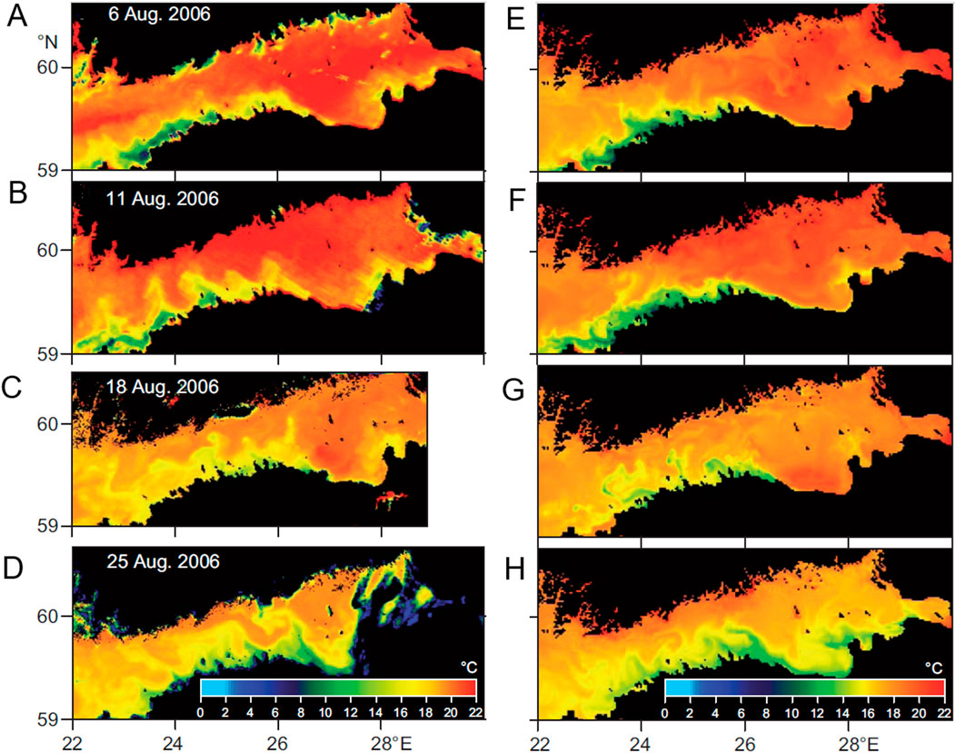
Figure 7. Sea surface temperature maps of the Gulf of Finland in August 2006: satellite imagery (A–D), model (E–H). Adopted from Laanemets et al. (2011).

5 Mesoscale dynamics

Mesoscale eddies are swirling patterns of currents of nearly circular shape capable of traveling as compact features over distances larger than their size. The Rossby deformation radius R_d is a key to defining the horizontal scale of mesoscale motions. It is the product of mean stratification strength (Väisälä-Brunt frequency) and depth divided by the Coriolis parameter, reflecting the effect of Earth rotation at a given latitude. Mesoscale eddies typically have a diameter a few times the R_d in the ocean and the marginal seas (Chelton et al., 2011). In the Baltic Sea, R_d = 4–8 km (Fennel et al., 1991); the stronger eddies have a diameter of up to 20 km and sometimes even more (e.g., Aitsam and Elken, 1982). Smaller-scale features, termed submesoscale, will be considered in the next Chapter.

Mesoscale eddies comprise an important intermediate part of the multitude of physical features in the sea, generated by the cascade of interacting physical processes, from the basin scales to the turbulent mixing scales. Within the basins, mesoscale eddies are formed by instability processes or forced baroclinic flows crossing the depth contours. Mesoscale eddies, which have a dominating geostrophic balance between the currents and horizontal pressure gradients (Rossby number Ro < 1), decay into ageostrophic (Ro > 1) submesoscale eddies that cause isopycnal and diapycnal mixing, with the help of internal waves and the thermohaline fine structure. Mesoscale eddies cause a “streaky” distribution of sea surface temperature and plankton variables (Garrett, 1983). Figure 8 presents a high-resolution satellite image of the cyanobacterial bloom in the region extending from Sweden in the west to Estonian Saaremaa Island in the east. The bloom is concentrated in the surface waters of the deep area between the coasts. The blooming is fed by the upward phosphorus fluxes from subsurface layers (weak in the shallow coastal regions) and by nitrogen fixation from the air. Within this basin-scale distribution, swirling mesoscale eddies are distinguished, visible by the surrounding submesoscale threads (elongated tracer stripes), where the bloom is more developed due to the enhanced nutrient and light availability.

Figure 8

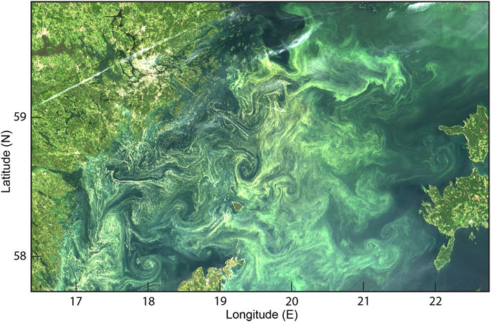
Figure 8. Cyanobacterial (primarily Nodularia spumigena) accumulations in the Northern Baltic Proper on 11 July 2005 as shown on MODIS Terra quasi true color image at 250 m resolution. Adopted from Kahru and Elmgren (2014).

Oceanic mesoscale eddies were discovered in the 1970s as persistent, slowly evolving eddy structures in current distributions (Koshlyakov and Grachev, 1973; McWilliams, 1976). The eddy currents are in geostrophic balance with density variations. Historical hydrographic data processing has often classified large temperature, salinity, and density anomalies as “suspect”. After discovering the mesoscale eddies, the abandoned density anomalies were used to construct worldwide maps of eddy occurrence (Dantzler, 1976). The Baltic Sea eddies were detected first mainly by density anomalies (Kielmann, 1978; Aitsam and Elken, 1982; Aitsam et al., 1984) since recording current meters used for the oceanic eddy detections were not available in large amounts. The validity of using the density-based geostrophic relations to determine mesoscale eddy parameters was confirmed by the PEX-86 experiment (Dybern and Hansen, 1989). An algorithm to detect the Baltic Sea eddies from hydrographic data was developed and tested by Reissmann (2005). Still, it is not widely used because of the relatively poor data coverage with densely-spaced CTD profiles.

Remote sensing is a valuable tool for identifying eddies over larger regions and studying their properties, as noted at the beginning of eddy science (Robinson, 1983). For the Baltic Sea, Horstmann (1983) produced a catalog of visible-range spectral and infrared thermal satellite images demonstrating water mass boundaries and mesoscale eddies. Bychkova and Viktorov (1988) outlined the geographical distribution of sea surface signatures of eddies. SAR (Synthetic Aperture Radar) images obtained from satellites allow the detection of a large number (thousands) of eddy-like surface slick structures (Karimova, 2012). By comparing the sizes of eddy structures in the Baltic, Black, and Caspian seas, they are scaled with the different values of local Rossby deformation radius. Unfortunately, due to the long interval between the snapshot SAR images, it has not been possible to identify the individual eddy’s life cycle events like growth, migration, interactions, and decay. In the oceanic eddy science, there is an interesting development to use machine learning algorithms for eddy detection from remote sensing data (Zhang et al., 2023; Zi et al., 2024), which has the potential to be implemented in the Baltic Sea studies.

Altimetry has a good dynamic presentation since it determines sea level gradients, enabling geostrophic calculations of ocean currents. The present altimetry is good for resolving oceanic eddies with diameters 100–200 km and a lifetime of more than 4 weeks (Chelton et al., 2007; Chelton et al., 2011) but too coarse for the Baltic Sea eddies with diameters 10–20 km and a lifetime of up to 10 days. In the Baltic Sea region, S3A and S3B altimeters have a repeat time of ground tracks of 13.5 days, and the interval between interleaved ground tracks is 27 km (Liibusk et al., 2020). With the anticipated improvement of altimetry coverage using SWOT sensors, there will be more dynamically meaningful data on the Baltic Sea currents, fronts, and eddies (Kupavõh et al., 2025).

Regarding the historical view on mesoscale variability, phytoplankton patchiness was found in the Baltic Sea in the 1970s. It stimulated the planning of an interdisciplinary study of mesoscale dynamics (ICES, 1979). The multi-ship (13 research vessels) 2-week patchiness study experiment PEX-86 was conducted during the spring bloom period (April - May) in the southern part of the Eastern Gotland Basin on a study grid of 20 x 40 nautical miles (Dybern and Hansen, 1989). The results established a close dependence of the patchy patterns of phytoplankton bloom with the geometry of eddies, jets, and fronts and associated saline stratification. A southward meandering jet was observed in the middle of the Hoburg Channel (Figure 9). To the east (left from the jet), a strong cyclonic eddy (Figure 9A) with a halocline elevation of about 15 m in the eddy center (Figure 9B) was observed, as also evident from the satellite image (Figure 9C). The center of the cyclonic eddy had a very homogeneous core from the surface down to about 30 m, suggesting an isolated water mass captured and transported from the origin of eddy formation (Elken et al., 1994). The phytoplankton spring bloom just started in the core of the eddy. An anticyclonic eddy was found to the west of the meandering jet. Both eddies had a diameter of 20 km and maximum rotational currents of 0.1 m s^-1.

Figure 9

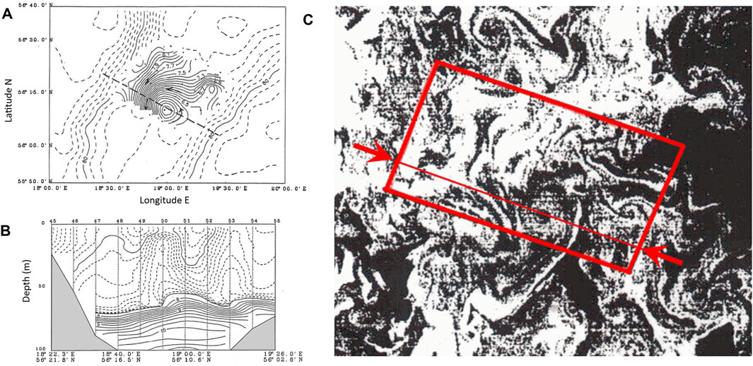
Figure 9. Observational data from 7 May 1986. (A) Map of the dynamic height of 10 dbar relative to 90 dbar, in dynamic cm (solid lines) and depth contours (dashed lines) around the map area. The position of the lower panel transect (B) is given by a heavy broken line. (B) A 40-mile salinity transect in the depth range 0–100 m, grid step between the profiles 4 nautical miles. The contour interval is 0.2 psu for solid lines and 0.02 psu for dashed lines. Modified from Elken et al. (1994). (C) Map of surface temperature mapped by LANDSAT TM channel 6. The red box shows the survey area of (A), and the thin red line shows the location of the transect (B). Modified from Dybern and Hansen (1989).

Advanced in situ observations of eddies (Zhurbas and Paka, 1999; Pavelson et al., 1999; Stigebrandt et al., 2002; Piechura and Beszczynska-Möller, 2004; Lass and Mohrholz, 2003; Lass et al., 2003; Voss et al., 2005; Elken et al., 2006; Lass et al., 2010; Lips et al., 2016; Krayushkin et al., 2023) are very valuable to complement the knowledge obtained from remote sensing and numerical modeling. Eddy-permitting models (Lehmann, 1995; Meier, 2007) have horizontal grid steps typically 4–6 km (2–3 nautical miles), comparable to the Rossby deformation radius. These models capture well the features of larger mesoscale eddies. Evaluation of different eddy-permitting models in reproducing long-term changes of stratification has been presented by Gröger et al. (2022). By refining the grid step to 1 km (0.5 nautical miles) and smaller, eddy-resolving models can handle smaller eddies (also in the coastal and shallow areas) and their interactions (Gräwe et al., 2013). However, these studies had too coarse horizontal resolution to focus on eddies. The models capable of resolving mesoscale and submesoscale eddies, with a resolution of 0.6 km or less, have been developed in recent years. These studies and the results will be analyzed in Section 6.

The properties of mesoscale eddies throughout their life cycle were studied by applying eddy detection algorithms to data from high-resolution numerical modeling. Vortmeyer-Kley et al. (2019) used three different eddy detection methods based on Eulerian and Lagrangian approaches to analyze the modeled current fields with a 0.6 km resolution. Over the 2-year modeling period, about 100,000 eddies were detected. In the variety of eddies, the lifetime of more than 2 days is covered by about 10% of eddies, but short-living eddy structures with lifetimes less than the inertial period (about 14 h) comprise about 40% of the eddy detections (however, it depends on the method used). On average, the eddies detected in the model have a diameter of 16 km, whereas the maximum diameter amounted to 40 km. Most eddies travel about 20 km, but migrations up to 80 km were also found. An independent example of long-time eddy travel for 33 days is given by Väli et al. (2017). Travkin et al. (2024) used the Baltic Sea Physics Reanalysis 1993–2020 with a 2 km resolution. Compared to the Rossby deformation radius, such a large grid step is known to smear out smaller eddies. However, similar to Vortmeyer-Kley et al. (2019), they found that most eddies have a diameter of 10–20 km, a lifetime of 2–3 days, and a sea level anomaly of 0.05–0.20 m in the eddy center.

Both the eddy detection studies indicated the dominance of cyclones at the surface and increased eddy activity during late autumn and winter, as was earlier found from in situ observations (Kõuts et al., 1990) and satellite SAR images (Karimova, 2012). Statistical detections of eddy diameters, lifetimes, and travel distances follow the results from observations. Persistent eddies observed at the surface are related to 10–20 m vertical excursions of halocline due to the geostrophic relations at low Rossby numbers. Eddies related to the isopycnal displacements in the thermocline have shorter lifetimes and smaller diameters.

Subsurface eddies have a belt of maximum vortex currents either in the halocline, the thermocline, or the intermediate layer between these layers. Intra-halocline lenslike eddies, identified from observations (Aitsam et al., 1984; Kõuts et al., 1990; Elken et al., 2006), have a double-convex shape of stretched isopycnals like the Meddies (deep lenses of Mediterranean water) in the Atlantic Ocean. Anticyclonic currents are concentrated around undisturbed deep isopycnals. These subsurface eddies have parameters similar to those of surface eddies. Identical to the Meddies, the Baltic subsurface eddies capture water mass from the location of eddy formation and transport it in the eddy nucleus throughout the ambient water mass with different properties. As another type of rotation, cyclonic subsurface eddies, with isopycnals contracted in the eddy nucleus, were observed after the Major Baltic Inflow (Zhurbas and Paka, 1999).

The eddy structures, found either in observational data or numerical results, need to be interpreted in terms of theoretical solutions, establishing the dependence between the parameters. In the ocean, the first observations of mesoscale eddies were interpreted as slowly moving linear Rossby waves (e.g., Koshlyakov and Grachev, 1973; Chelton et al., 2011) existing within the Boussinesq approximation due to the variation of the Coriolis parameter by latitude (beta effect). In the Baltic Sea, the topographic effect on mean vorticity change largely dominates over the vorticity variation due to the change in latitude. This favors the interpretation of eddies in connection with coastal trapped or topographic waves (Walin, 1972; Aitsam and Talpsepp, 1982; Pizarro and Shaffer, 1998; Stipa, 2004; Holtermann et al., 2014), although true topographic waves appear in the bottom layers of sloping topography. Theoretically, eddies may be generated by the baroclinic instability of large-scale mean currents. However, this interpretation in actual situations is complicated because of disturbing factors like low gradients in the mean currents and the topographic variations that may modify the generation mechanism.

The nature of Baltic Sea mesoscale eddies can be divided by generation mechanisms - forced or random eddies. Forced eddies occur due to wind action when a variable larger-scale flow crosses the (abruptly changing) depth contours or goes past the coastal capes. Their size is determined mainly by topographic features and stratification. Under similar weather forcing, the eddies are formed in nearly the same locations. Random eddies are generated due to the baroclinic and barotropic instability of disturbances that may grow in a sheared flow. Their size is a few times the Rossby deformation radius. During their life cycle, from formation to decay, eddies may migrate as compact features over significant distances.

Eddies comprise a significant chain in the energy and vorticity cascade of multi-scale physical transport and mixing processes (Meier et al., 2006; Reissmann et al., 2009), enhancing them at large spatial and temporal scales. Mesoscale eddies cause relatively high values of lateral diffusion coefficients, from 500 to 2000 m² s^-1 (Zhurbas et al., 2008; Burchard et al., 2017), while in the submesoscale models, the diffusion coefficient calculated by the Smagorinski formula is below 10 m² s^-1. Depending on their generation mechanism and location, the eddies create heterogeneities of flow and tracers at smaller scales. The specific role of eddies in the Baltic Sea may be depicted as (a) eddies transport in their nucleus the trapped water from the region of their formation, and/or (b) eddies have a specific fluid dynamics regime of diapycnal and isopycnal motions and mixing, supporting thermal and biological niches different from ambient waters, enhancing or suppressing the growth of thermal and/or biogeochemical anomalies (e.g., Vortmeyer-Kley et al., 2019).

6 Submesoscale dynamics and mixing

Submesoscale dynamics cover motions with a scale smaller than Rossby’s deformation radius (mesoscale) and larger than the thermohaline fine structure and turbulent mixing. Oceanic submesoscale patterns have a scale of 200 m–20 km (Taylor and Thompson, 2023). Submesoscale variability is seen on the sea surface as squirts and striped structures of temperature or other scalar fields, often curved along mesoscale eddies and fronts. While geostrophic balance dominates the mesoscale motions, ageostrophic effects are important in submesoscale dynamics. Oceanic submesoscale features significantly affect large-scale flows’ transport, mixing, and dissipation (McWilliams, 2019). Knowledge of submesoscale dynamics has advanced during the recent decade thanks to the rapid developments in observation and modeling techniques. Earlier knowledge on thermohaline intrusions (Ruddick and Richards, 2003) has been merged into the submesoscale concept.

In the Baltic Sea, the submesoscale processes with high values of Rossby number have spatial scales across the intrusive thread of less than 5 km and time scales of a few days (Lips et al., 2016; Väli et al., 2017; Chrysagi et al., 2021; Salm et al., 2023). Observational findings of the Baltic Sea submesoscale are provided by modern high-resolution observational techniques that involve surface transects using FerryBox systems, profiling buoy installations observing the water column, ScanFish-type towed sensors, undulating underway sensors behind the ship, and autonomous glider missions. The results revealed that horizontal wavenumber temperature spectra at scales from 0.5 to 10 km have a slope −2 characteristic of ageostrophic sub-mesoscale motions (Lips et al., 2016). For example, by 10-km-long glider missions in the Gulf of Finland (Figure 10), basin-scale current (apparent by salinity and density slopes) had in its core submesoscale water mass variations evident of temperature anomalies along constant density; they were also characterized by the thread pattern of the currents (Salm et al., 2023). The results indicate that submesoscale frontal dynamics contribute to the energy cascade.

Figure 10

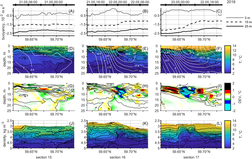
Figure 10. (A–C) Buoyancy along the glider transect at 3, 15, and 25 m depth on 20–23 May 2018. (D–F) Temperature distributions (black contours with a step of 1°C) as a function of depth (0–25 m) overlaid with white contours marking the relative geostrophic velocity with a step of 2.5 cm s^-1 on 20–23 May 2018. The sampling timeline is at the top of the columns. The left side of a subplot is located closer to the coast and presents the southern part of the section. The distance between the ticks presenting latitude is about 2.7 km. (G–I) Temperature deviations as a function of pressure along the glider section on 20–23 May 2018. Black contours mark potential density anomaly with a step 0.1 kg m^-3. (J–L) Isopycnal temperature distributions (black contours with a step of 1°C) along the glider section on 20–23 May 2018. From Salm et al. (2023).

Numerical models, resolving the submesoscale with a grid step of 0.6 km or less, enable comprehensive dynamical analysis of the terms and balances in the hydrodynamic equations. A useful approach to handle the submesoscale structures is to calculate “gradient” characteristics. The Rossby number (Ro), as a ratio of the vertical vorticity component to the Coriolis parameter, is one of the main objects of such analysis, distinguishing between the geostrophic mesoscale (Ro < 1) and ageostrophic submesoscale (Ro > 1) regimes. Other quantities to explain the fate of threads include the horizontal divergence of currents, the horizontal buoyancy gradient, vertical velocity, Richardson number, frontogenetic strain rate, thermohaline spice (defined as the ratio of temperature and salinity variations to yield unchanged water density), but also kinetic energy and potential energy anomaly (Väli et al., 2017; Onken et al., 2020; Chrysagi et al., 2021; Väli et al., 2024).

A study by Chrysagi et al. (2021), based on high-resolution modeling supported by satellite images and CTD transects, revealed that cold submesoscale filaments were formed in a thermal front in the Eastern Gotland Basin (Figure 11). The temperature drop of about 4°C was formed due to (1) advection of warmer waters from the south along the eastern coast by cyclonic circulation and by (2) cooling the surface of deeper areas by upwelling near Gotland island and advection of colder water from the north. The filaments had large horizontal density gradients, strong surface convergence of flows, and high vertical velocities. Submesoscale dynamics created high heterogeneity of the mixed layer depth. The locally reduced mixed layer depth was maintained even during storm events due to the submesoscale restratification. The interaction of near-surface turbulence and submesoscale restratification results in strong and highly efficient mixing inside the submesoscale fronts.

Figure 11

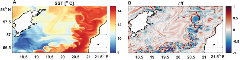
Figure 11. Maps of the surface dynamics in the Eastern Gotland Basin (between the Gotland island on the west and the Latvian coast on the east) on 19 October 2017. (A) Sea surface temperature (SST), (B) Rossby number, i.e., relative vorticity normalized by the Coriolis frequency. Modified from Chrysagi et al. (2021).

Model studies of the eddy statistics over annual or longer periods (Vortmeyer-Kley et al., 2019; Väli et al., 2024) have revealed the dominance of cyclonically curved submesoscales over anticyclonic. Preference for cyclonic vorticity has also been pointed out by shorter model studies (Väli et al., 2017; Onken et al., 2020; Zhurbas et al., 2022) and SAR satellite images (Karimova, 2012). It was also found that there was a higher intensity of mesoscale eddies and submesoscale features during the winter compared to the summer. Väli et al. (2024) concluded that the vertically averaged kinetic energy (including that of meso- and submesoscales) is about 70 cm² s^-2 in December–January and is reduced to 30 cm² s^-2 in June–July. For the observational background, deep-layer available potential energy was calculated from the mesoscale CTD surveys conducted in 1984–1992 in the Eastern Gotland Basin. Analysis of vertical excursions of isopycnals and the mean Väisälä frequency within the survey areas revealed available potential energy in winter above 70 cm² s^-2 and in summer below 20 cm² s^-2 (Elken, 1996).

The geographical and seasonal distribution of eddy activity has been studied by Väli et al. (2024) using the probability distribution of the Rossby number. Ranges with absolute values in [0, 0.25], [0.25, 0.5], [0.5, 1.0], and [1.0, …] were selected to indicate no eddy activity, weak, moderate, and strong (submesoscale/ageostrophic) eddy activity, respectively. Figure 12 depicts the distribution of weak and moderate eddy activity over the whole study period of 2010–2018. While weak eddy activity represents a linear regime of vortexes with low impact on mixing, moderate eddy activity corresponds to the significant non-linear effects in vortex motions, approaching the ageostrophic submesoscale regime, which may be accompanied by curved threads at Ro = 1. High values of eddy activity are found in the areas of high temporal variability of salinity (Figure 6B). In addition to the frontal regions between the basins and the Western Baltic transition area, high eddy activity is also found in the deep-water path from Stolpe Channel to the Gdansk Basin (Figure 5). Another eddy-active region is along the south-westward brackish water pathways from the Gulf of Finland and the Bothnian Sea along the Swedish coast of the Baltic Proper. The Gulf of Finland is entirely an eddy-active region. Supposedly, high lateral salinity and density gradients favor the generation of eddies due to instabilities; on the other hand, the eddies mix the water masses and reduce the gradients. Although it has been noted that eddies and filaments are often formed during the upwelling processes (Figure 7), the geographical distribution of upwelling occurrence obtained from remote sensing and modelled data (Lehmann et al., 2012) is not directly reflected in the distribution of the Rossby number.

Figure 12

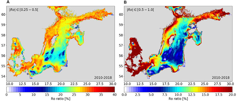
Figure 12. Spatial distributions of the occurrence of the weak (Rossby number ranges 0.25 < |Ro| <0.5, (A)) and moderate 0.5 < |Ro| <1, (B) eddy activity in the surface layer for the period 2020–2018. Modified from Väli et al. (2024).

Wind forcing increases the kinetic energy of the surface layer and the whole water column; however, the activated mesoscale and submesoscale motions lag behind the wind speed variations (Väli et al., 2024). In the mechanistic models of coupled basins, wind energy transfer and vertical mixing are governed by turbulence models based on balances of turbulent kinetic energy and its dissipation. The mixed layer dynamics are usually properly simulated in these models. Still, in the deeper layer, penetration of direct wind forcing tends to be too small to explain the observed changes in stratification. A common approach to overcome too low mixing is to include additional mixing terms in the turbulence coefficient, due to the breaking of internal waves. According to Stigebrandt (1987), the extra term is proportional to the inverse of the Brunt-Väisälä frequency. As an example, simulating the end of the enhanced stagnation period 1985–1994, with only a few deep inflows (Figure 13A), Axell (2002) obtained that the 1D model simulation (Figure 13B) reasonably fits the observation only in cases when mixing by internal waves is included. The same additional deepwater mixing is also used in three-dimensional models (Meier, 2001). However, this is a bulk formulation to simulate the overall vertical mixing in the basin. Vertical mixing is intensified on the slopes of the basins where isopycnals of the halocline intersect the bottom slope. Enhanced mixing may be generated due to breaking internal waves arriving at the slope area from the basin interior, by shear instability of slope or rim currents flowing above rough topography, and other processes (Axell, 1998; Zhurbas and Paka, 1999; Holtermann et al., 2014; Muchowski et al., 2023). A boundary-layer water mass with anomalous thermohaline properties is spread to the basin interior through lenslike eddies and intrusions. Intrusion-free deep layers of the basin interior are observed about 1 month after the formation of slope anomalies (Kõuts et al., 1990; Elken, 1996; Holtermann et al., 2014).

Figure 13

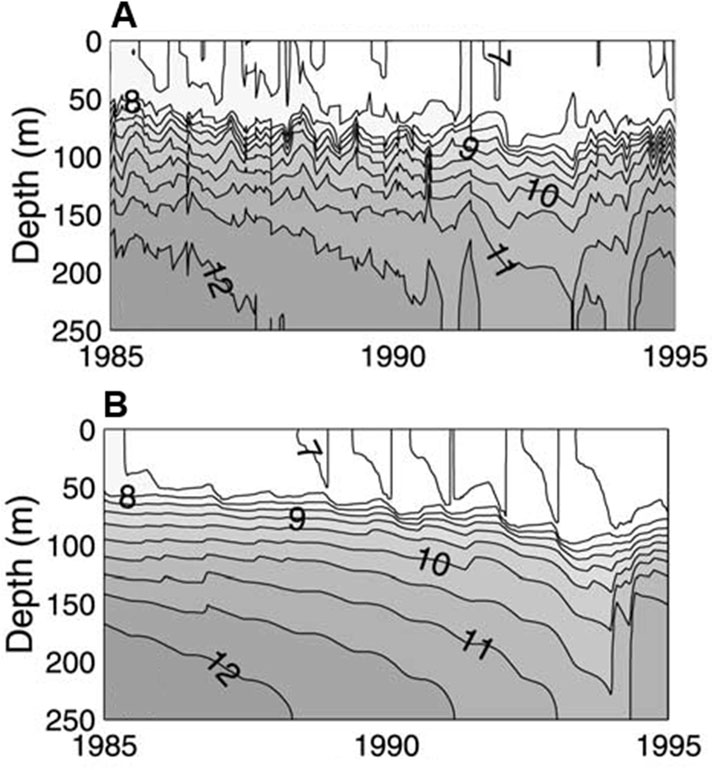
Figure 13. Observed salinities from the central Baltic Sea (A) and calculated salinities (B) by adding internal wave energy and Langmuir circulation. Adopted from Axell (2002).

There are already many examples of how submesoscale features, generated by a wide range of instability processes at the surface, in the pycnoclines, and in the bottom boundary layer (McWilliams, 2019), participate in the energy cascade from wind and thermohaline forcing to microscale turbulence. However, this research field is far from knowledge “saturation” and further studies are needed.

7 Discussion

The mechanistic models of connected sub-basins give realistic results without resolving the internal sub-basin structures. The mechanistic models resolve the vertical dimension, identify the connection between the sub-basins through the straits, and apply simplified strait flow models. The energy flow from atmospheric forcing ends up in the deeper layers, which are parameterized based on observations during stagnation periods. From model simulations, the Baltic Sea seems to be a strongly forced and damped system. Through winds, heat fluxes, saline water inflow, and river runoff, boundary layer forcing generates currents and eddies and is damped through friction. A well-known observation is, for example, the inertia oscillations that are damped within some oscillation periods (Gustafsson and Kullenberg, 1936). It has not been observed that the system can shift to different stable flow regimes, as discussed for the ocean starting from Stommel (1961). However, the possibility of different stable flow regimes in the Baltic Sea needs further consideration. For example, from a highly estuarine circulation with a strong deep-water inflow to a lake circulation with complete overturning circulation.

Turbulent flow involves a multitude of eddies at various scales, some on different scales. This was already illustrated in a drawing by Leonardo da Vinci (1,507–1,509) and described in the book by Cushman-Roisin and Beckers (2011), page 132). Today, the strong eddy structure in the Baltic Sea can easily be observed from satellite data, e.g., in Figure 8, and its various scales are discussed in Chapters 5 and 6. Eddies and related currents are pervasive throughout the ocean and a part of the energy flow in the marine system (McWilliams, 2019). From the basin scale, the energy flows through mesoscale, sub-mesoscale, and microscale, where the energy dissipates. The way the mechanical energy flux is related to the deep-water mixing is almost unknown and needs further studies.

The relevant time scale for the mechanistic models is the time it takes to fill a cascade of sub-basins, i.e., the ratio between the volume and the amount of in- or outflow. The propagation time of saline water entering after the Major Baltic Inflow was observed in different deep basins for up to a year (Liblik et al., 2018). The time scale for eddies and submesoscale intrusions along the isopycnals is generally much less, typically 10 days or less.

The mechanistic models assume that the subbasins are horizontally quasi-homogeneous. It means that if the actual contrasts of tracers (e.g., temperature, salinity) within the basin arise (including between the coastal and offshore regions, Figures 7, 11), they are smeared out by meso- and submesoscale processes by a time scale of about 1 month which is a reasonable time frame of the well-working box models. At the same time, the tracer contrasts between the subbasins are governed by meso- and submesoscale frontogenesis, restoring the gradients against mixing. Meandering fronts contribute to the water and tracer transport by shedding the mesoscale eddies and intrusive submesoscale threads. There are indications that meso- and submesoscale mixing contributes more than 90% of the actual lateral mixing. Still, effects of “negative” viscosity and diffusivity also may occur, i.e., during the formation of jet currents and restratification.

Recent years have witnessed a rapid development of ocean descriptions based on machine learning (ML) approaches (de Burgh-Day and Leeuwenburg, 2023). Instead of using the basic laws in physics, like mechanistic coupled basin models and fully three-dimensional numerical models, these ML models are based on patterns found from big data using some feature extraction method. In the Baltic Sea, ML methods have been used for short-term prediction of extreme sea-level (Bellinghausen et al., 2025), identification of sea surface circulation patterns (Barzandeh et al., 2024), and finding environmental drivers of phytoplankton blooms (Berthold et al., 2025). While data-driven ML forecasts are computationally very efficient, their performance deteriorates when used outside the data training period, for example, in future climates. In this context, mechanistic and numerical models are considered more robust for variations in the ocean mean state.

There are examples of combining machine learning with physics-based numerical modeling (Sonnewald et al., 2021; Bracco et al., 2025) to improve the parametrization of sub-grid processes and applying data assimilation, especially regarding the submesoscales. It is a promising approach, but the applications of the Baltic Sea cannot yet be found. Presently, there are more than ten numerical hydrodynamical models used in the Baltic Sea for different purposes, like short-term physical process studies (e.g., Burchard et al., 2009; Holtermann et al., 2014; Väli et al., 2017), past climatic changes of the physical system (Schimanke et al., 2012; Radtke et al., 2020), operational forecasting (Golbeck et al., 2015; Kärnä et al., 2021), and climate projections (Meier et al., 2022). State-of-the-art numerical modelling of the Baltic by different models and their setups has been compared and reviewed by Placke et al. (2018) and Gröger et al. (2022). Models with submesoscale resolution are still rare, as shown in Chapter 6, and due to the high computational demand, they cover only short periods of calculation.

Future research directions in modelling are expected to enforce true submesoscale-resolving models capable of decadal and centennial model runs, with applied improvements for the non-hydrostatic vertical momentum equation and improved parametrizations from sub-grid scale processes, as well as waves and ice, incorporating the knowledge from observations through machine learning. Longer time scales could be covered by the models of reduced complexity tuned against high-resolution data, either by numerical models of lower resolution or the mechanistic models integrated over the basins.

The large differences in the time scale of basin filling (about 1 year), basin isopycnal through-mixing (>1 month), and eddies (<10 days) illustrate that it is reasonable to assume horizontally homogeneous sub-basins when working on longer time scales with support from the approaches used in the Knudsen theorem. Joint use of the different methods involved in the coupled basin mechanistic models and eddy-resolving models could help understanding the Baltic Sea Earth system, for example, when calculating the ensemble means during climate change studies (Meier et al., 2018).

8 Summary and conclusion

In the present review, we have considered the water exchange in the Baltic Sea based on a historical view of research approaches from basin scales to submesoscale. Mechanistic models of connected sub-basins have been applied in a series of studies starting from the Knudsen theorem. In this class of models, the basin and sub-basin structure was assumed to be horizontally homogeneous, a reasonable assumption on the climate time scale. In parallel, many studies were devoted to mesoscale and submesoscale eddy structures that are highly variable in time and space. These eddy structures are a natural part of the ocean and coastal seas, transforming the large-scale energy through a cascade into smaller scales.

The conclusions could be summarized as follows:

• The mechanistic models and three-dimensional submesoscale approaches complement each other.

• The mechanistic models are useful for interpreting large-scale effects of submesoscale processes; they also allow more numerical experiments and longer modeling periods for climate and long-term environmental studies than three-dimensional eddy-resolving models.

• The submesoscale approaches may guide parametrizations of exchange between the sub-basins and within them.

• Recent submesoscale studies suggest localized eddy-rich regions: Arkona Basin, Gulf of Finland, Irbe Strait, Åland Sea connections, and several coastal areas.

In the coming Baltic Earth phase 2.0, several questions still need new research efforts. A better understanding of the flow of mechanical energy from large-scale forces is needed through basin scale, mesoscale, submesoscale, and microscale. These studies are necessary for the many applied aspects, like offshore building of wind farms and other building activities that may reduce the energy flow, as well as for scenario studies related to other man-made activities under a changing climate.

Author contributions

JE: Writing – review and editing, Writing – original draft, Investigation, Conceptualization, Methodology, Project administration, Formal Analysis. AO: Writing – review and editing, Methodology, Formal Analysis, Investigation, Writing – original draft, Conceptualization.

Funding

The author(s) declare that financial support was received for the research and/or publication of this article. This work was co-funded by the European Union and the Estonian Research Council via the project TEM-TA38 (Digital Twin of Marine Renewable Energy).

Acknowledgments

This work is part of the Baltic Earth Working Group on Philosophical Views of Baltic Earth and Science. The first version of this paper was partly presented during the 5th Baltic Earth Conference, Jūrmala, Latvia, from 13 May to 17 May 2024, and partly during the Special Baltic Earth Colloquium – achievements, thanks and future challenges, Hamburg, Germany, 4 February 2025. We want to thank the organizer for these two meetings, particularly Marcus Reckermann, for his long service within the Baltex/Baltic Earth program.

Conflict of interest

The authors declare that the research was conducted in the absence of any commercial or financial relationships that could be construed as a potential conflict of interest.

Generative AI statement

The author(s) declare that no Generative AI was used in the creation of this manuscript.

Publisher’s note

All claims expressed in this article are solely those of the authors and do not necessarily represent those of their affiliated organizations, or those of the publisher, the editors and the reviewers. Any product that may be evaluated in this article, or claim that may be made by its manufacturer, is not guaranteed or endorsed by the publisher.

References

Aitsam, A., and Elken, J. (1982). Synoptic scale variability of hydrophysical fields in the Baltic Proper on the basis of CTD measurements. Elsevier Oceanogr. Ser. 34, 433–467. doi:10.1016/s0422-9894(08)71254-6