A conceptual model framework for integrating monitored-unmonitored and surface-subsurface flow contributions to the Baltic Sea

Understanding the total water flows and pollutant loads to the Baltic Sea is important for effective coastal-marine ecosystem management. Current assessments often overlook the unmonitored flows and submarine groundwater discharge (SGD). This study proposes and outlines a conceptual modelling framework for overcoming this common neglect by integrated quantification of (1) the monitored surface water flows, and the unmonitored (2) surface water flows and (3) SGD from land to the Baltic Sea. The study outlines how unmonitored runoff and SGD can be estimated by various quantification approaches based on commonly available hydro-climatic, hydrogeological, and other characteristic catchment data. It also describes how modules for the different monitored and unmonitored discharge components are linked and should be integrated in modelling to total annual, seasonal, or finer-resolved water flows to the Baltic Sea, and analogously also in other coastal regions around the world. Though quantitative modelling remains ongoing, the conceptualization opens pathways to improve assessments and management of freshwater flows and associated pollutant loads to the Baltic Sea.

1 Introduction

The Baltic Sea is a unique marine ecosystem highly sensitive to changes in water input from its surrounding catchment area (Saraiva et al., 2019). However, the Baltic Sea is also highly susceptible to pollution and nutrient loading from its extensive drainage basin, which includes numerous countries and diverse landscapes. This pollution is intensified by both natural processes and anthropogenic activities, leading to significant environmental concerns such as eutrophication and habitat degradation (Reckermann et al., 2022; Vigouroux et al., 2021). To understand, predict and control the major waterborne pollution from land to the Baltic Sea, it is important to identify the pathways of the inland water to the sea and quantify the water flow through them. The task is complex due to the varied sources and types of water discharge to the sea, including both monitored and unmonitored flows (Figure 1).

Figure 1

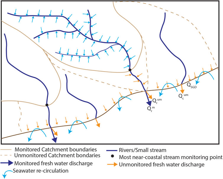
Figure 1. The different monitored and unmonitored pathways of water from land to sea. Straight arrows at and across the coastline show monitored (blue) and unmonitored (orange) freshwater discharges to the sea. Blue lines within the catchments show rivers and streams. Arrows within the catchments and at the coastline show the diffuse groundwater flow field (modified from Destouni et al. (2008). Flow components include: Q_r^m–monitored river flow; Q_r^um–unmonitored portion of river flow from partly monitored catchments; Q_c^um–flow from completely unmonitored catchments; Q_SGD–submarine groundwater discharge. All terms are defined in detail in Section 2.

Hydrological catchments of coastlines are often outside the scope of the systematic monitoring that is usually conducted in major rivers. The significance of these unmonitored flows has been highlighted in previous studies, such as those by Hannerz and Destouni (2006), who showed the extent of highly populated, even though small, unmonitored coastal catchments, and Destouni et al. (2008), which showed the substantial contributions from such small unmonitored catchments to the overall nutrient and pollutant loading of the Baltic Sea. These unmonitored areas, with their commonly high population densities and significant agricultural activities around the Baltic region, can disproportionately affect coastal water quality. Spatial characterization of these catchments must consider a complex interplay between land use, population pressures, and hydrological responses, necessitating an integrated approach to water management.

Hydrological monitoring often excludes smaller coastal catchments, even though these contribute significantly (>10%) to pollutant loads entering the Baltic Sea (Destouni et al., 2008; HELCOM, 2023). Moreover, submarine groundwater discharge (SGD), the flow of water from land into the ocean through the seabed, is often assessed separately from surface water flows, despite its importance. This manuscript proposes and outlines an integrated conceptual framework that combines monitored flows, unmonitored runoff, and SGD to quantify total freshwater fluxes to the Baltic Sea, thereby addressing these overlooked pathways. This approach facilitates future modelling of pollutant loading and offers targeted management solutions.

2 Overview and description of the conceptual model

2.1 Overview

The framework quantifies total water flows to the Baltic Sea through two primary modules: the Monitored flow module and the Unmonitored flow module, which encompass four flow pathways (Figure 1):

1. Monitored river flows (Q_r^m)

2. Unmonitored part of the monitored river flow (Q_r^um)

3. Entirely unmonitored river flow in the unmonitored catchment (Q_c^um)

4. Unmonitored groundwater discharge (Q_SGD)

The two modules - Monitored flow module and Unmonitored flow module - are explained in the following sections. Each module addresses specific components of hydrological inputs using various methodologies to ensure an overall assessment. The methodologies and processes for each module are also elaborated in the subsequent sections to provide a detailed understanding of the conceptual framework and its application to assessing the hydrological contributions to the Baltic Sea. Figure 2 shows the overall workflow for the conceptual framework.

Figure 2

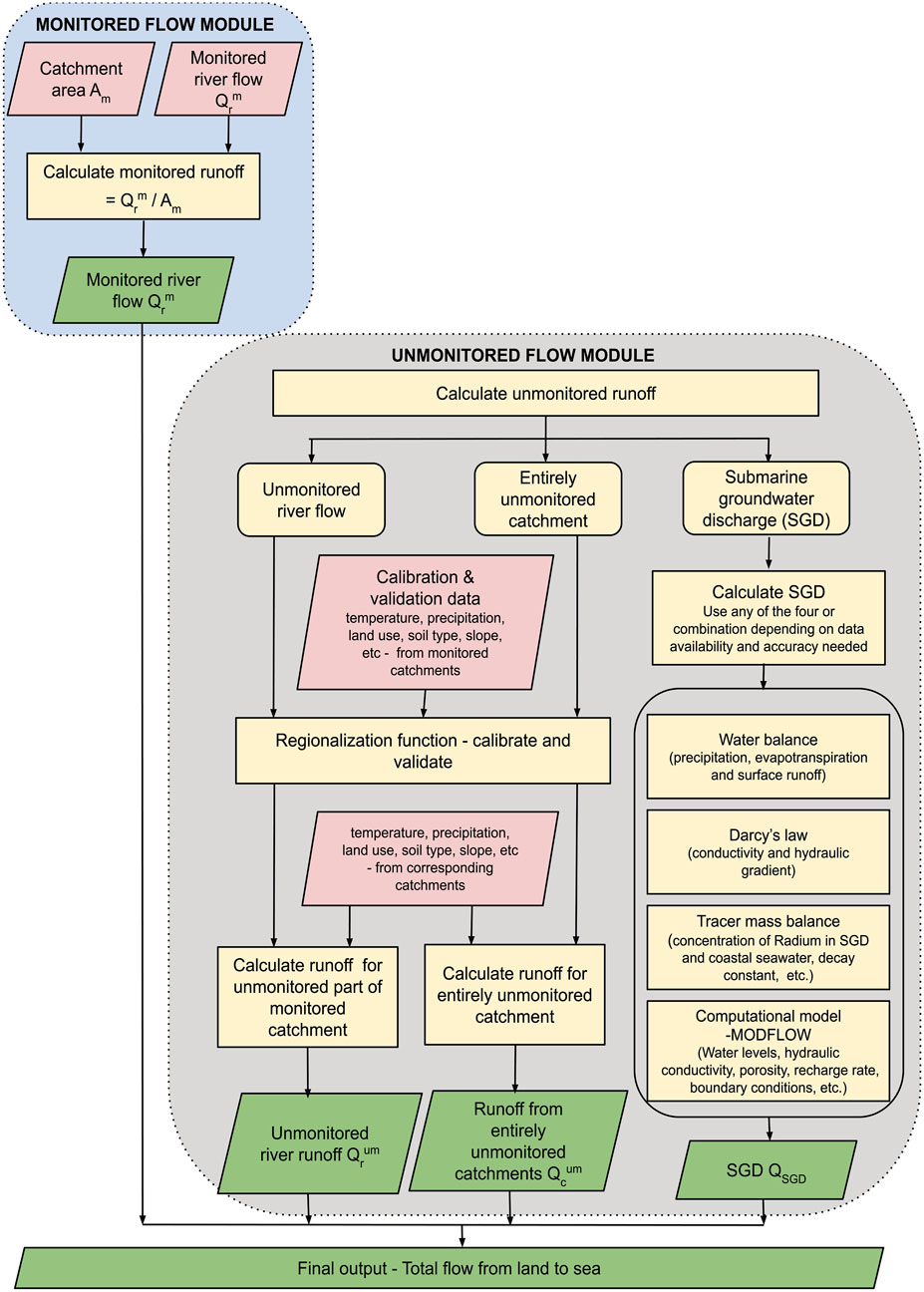
Figure 2. Conceptual model workflow.

2.2 Monitored flow module

The runoff from monitored areas to and through the streams and rivers of coastal catchments is captured in regular river discharge measurements and is termed monitored river flow ($Q_r^m$). The average runoff (R) per unit area of the contributing monitored catchment is obtained using Equation 1, by dividing the measured discharge by the contributing catchment area.

$R=Q_r^m/A_{m }(1)$

where A_m is the catchment area that contributing water to the monitored volumetric river flow (discharge, $Q_r^m$). The input data needed for Equation 1 are summarized in Table 1. Catchment area information covering the Baltic Sea drainage basin is detailed in Hannerz and Destouni (2006). Associated monitored river discharge data can be obtained from the measurement stations operated by national meteorological and hydrological agencies (e.g., SMHI in Sweden, FMI in Finland) or global runoff databases like the Global Runoff Data Centre (GRDC) and the Global Land Data Assimilation System (GLDAS).

Table 1

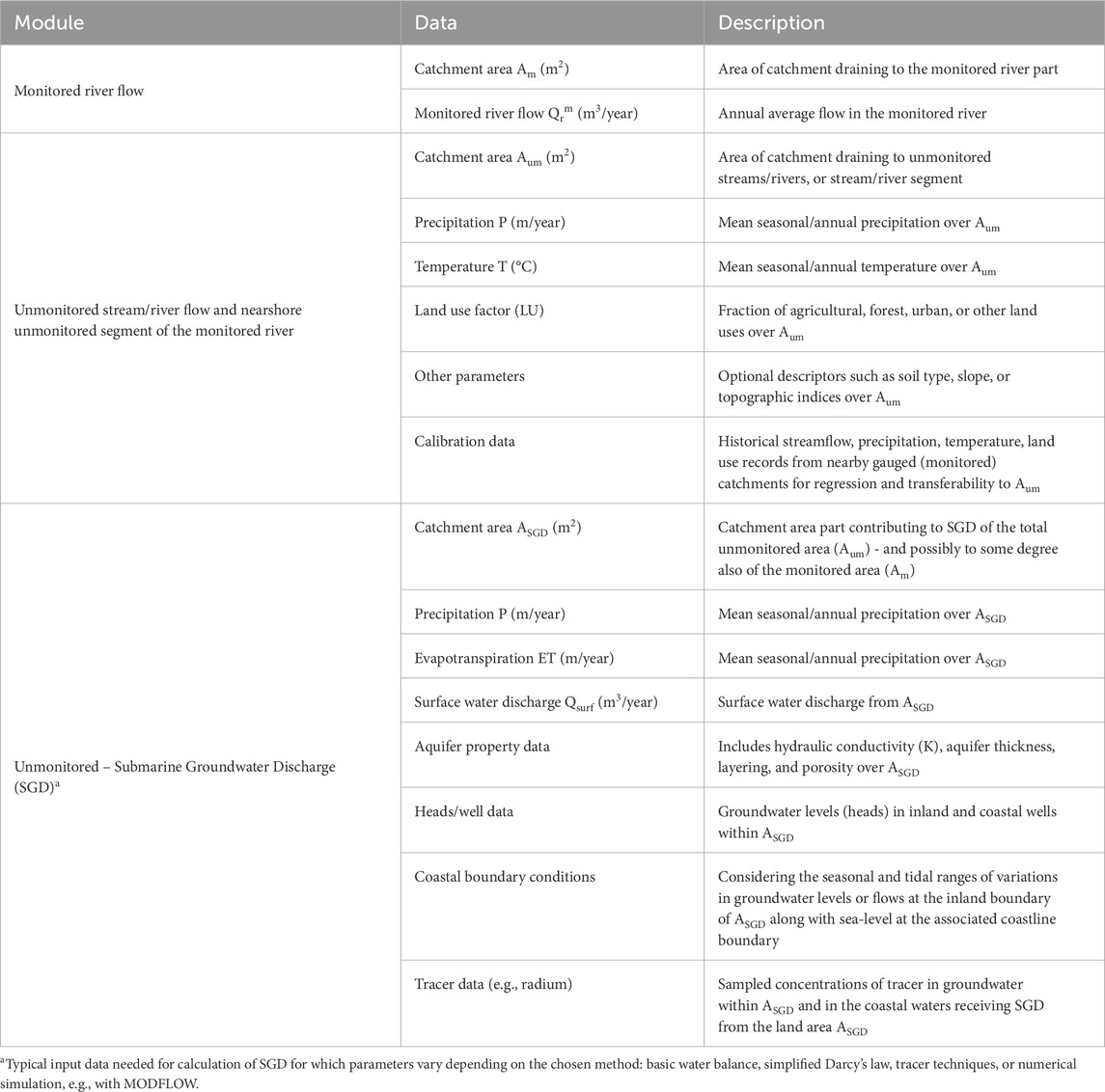
Table 1. Input data needed for calculating runoff from monitored and unmonitored catchments.

2.3 Unmonitored flow module

The unmonitored flow module addresses the runoff and groundwater contributions that are not systematically measured. This module comprises two submodules. The first submodule calculates the unmonitored portion (Q_r^um) of the river flow that is partly monitored (with the monitored part being Q_r^m). Often, the monitoring stations are not located at the actual river discharge points to the sea (i.e., they are not located at the coastline), leaving a portion of the catchment, downstream of the Q_r^m measurement stations, unmonitored (i.e., a nearshore unmonitored segment) even though the main river itself is measured further upstream. The second submodule estimates the flow from entirely unmonitored coastal catchments, which includes both unmonitored river flow (Q_c^um) and SGD (Q_SGD) (Figure 1).

2.3.1 Unmonitored river flow

If a catchment is unmonitored, that is, without any systematic monitoring of its stream and river flows, these flows and the associated runoff need to be calculated in other ways, as do also the nearshore unmonitored segment flows. This can be done through regionalization approaches (transferring hydrological information from monitored catchments to unmonitored catchments), deriving statistical or machine-learning relationships from nearby or analogous monitored catchments and applying these to the unmonitored areas (He et al., 2011; Prieto et al., 2019). One of the earliest applications of regression-based regionalization can be traced back to (Nash, 1960), who derived empirical relationships between unit hydrographs and various catchment characteristics. Since then, numerous studies have expanded upon this approach to estimate rainfall–runoff model parameters and streamflow statistics for unmonitored catchments. In this approach, the unmonitored river/stream discharge Q_i over an unmonitored catchment area or catchment area part A_um can be modelled as a linear function of precipitation (P_i), temperature (T_i), and a characteristic land use factor (LU_i) over that area (Equation 2).

$Q_i=\alpha +{\beta }_1*P_i+{\beta }_2*T_i+{\beta }_3*{LU}_i+(2)$

where Q_i is the discharge in the unmonitored stream/rivers or stream/river parts of the unmonitored catchment (part) i, P_i is the mean precipitation, T_i is the mean temperature, LU_i is the land use factor (e.g., fraction of agricultural or forested area) over the area A_um, and α and β are catchment-characteristic coefficients with relevant units for the equation result to yield the correct resulting units of Q (volume of water per time). Depending on data availability, additional parameters such as soil characteristics or topographic indices can also be incorporated (Addor et al., 2017).

When data are scarce, a power-law relationship that links runoff to the streams/rivers of the unmonitored catchment area (part) A_um-i​ can be used (Mazivanhanga et al., 2024) as in Equation 3.

$Q_i=b_i*A_{um-i}^c(3)$

where Q_i is the stream/river discharge in the unmonitored catchment (part) i, A_um-i is the corresponding catchment area, and b and c are coefficients with relevant units for the equation result to yield the correct resulting units of Q. Numerous studies indicate that catchment area frequently is the principal explanatory variable in both simple and multi-variate regression equations for streamflow prediction (Kuentz et al., 2017; Westergard et al., 2004). This approach remains popular because area data are readily obtainable (from digital elevation models or published catchment boundary maps), making Equation 3 an initial step in unmonitored catchment hydrology. However, many of these studies emphasize that local climatic conditions, geological heterogeneity, and land use factors can alter the exponent α or require the inclusion of additional parameters to improve predictive accuracy.

The equations (Equations 2, 3) can be calibrated using observed values from nearby monitored catchments and validated against an independent data subset to ensure generalizability (Wagener et al., 2004). This often involves splitting the available monitored catchments data into calibration and testing parts, to ensure that the derived coefficients do not merely reflect site-specific anomalies. Table 1 summarizes typical data needs, including historical streamflow records, precipitation, temperature, and catchment descriptors (land use proportions, slope, and area). A key limitation lies in the assumption that relationships calibrated at monitored sites transfer reliably to unmonitored catchments. Additionally, localized factors such as variable soil properties or extreme weather events can introduce further uncertainties. Complementary use of machine-learning models, such as random forests, can be used to improve performance by capturing complex, nonlinear interactions (Asadollahi et al., 2024). However, specific implementation details of such methods lie beyond the scope of the current study. Regardless of the chosen approach, updating the assessment of unmonitored river flow with new data helps refine the accuracy of unmonitored runoff estimates.

2.3.2 Unmonitored SGD

Fresh groundwater that flows directly into the sea from the SGD-contributing area part A_SGD of the total unmonitored catchment area (A_um above) - and possibly to some degree also of the monitored area (A_m above) - can substantially influence coastal water budgets and nutrient transport (Santos et al., 2021). The total SGD may be entirely fresh, partly saline, or recirculated seawater. Multiple techniques exist for estimating SGD. Four commonly applied methods are outlined here, each chosen to address varying degrees of hydrogeological complexity, data availability, and spatial scales typical of Baltic Sea catchments:

1. Basic water balance approaches

2. Simplified use of Darcy’s law

3. Tracer techniques

4. Numerical modelling, exemplified here by MODFLOW (USGS, 2024).

The following sections describe these methods, and Table 1 outlines typical data requirements.

2.3.2.1 Basic water-balance approach

A simple method interprets the freshwater part of SGD as the residual of a large-scale catchment water budget. The water balance equation for a catchment to estimate SGD can be written as (Burnett et al., 2006):

$Q_{SGD-f}/A_{SGD}=P-ET-Q_{surf}/A_{SGD}(4)$

where Q_SGD-f is the freshwater part of total SGD, P is precipitation, ET is evapotranspiration, and Q_surf is the surface water discharge, e.g., with these fluxes regionally estimated or modelled, over the SGD-contributing area $A_{SGD}$. Over a long time period, it may be reasonable to assume that the water fluxes in Equation 4 are balanced so that the average storage change (ΔS) is negligible. This approach has been used in many studies estimating SGD at large scales (Gwak et al., 2014; Russo et al., 2023). Its main advantage lies in its simplicity and reliance on readily available hydro-climatic data, making it especially suitable for preliminary assessments in data-scarce regions. However, it has limitations when ΔS≠0/for example, due to transient pumping or seasonal and interannual variability. Additional uncertainty arises when total SGD is required including recirculated saline water in addition to the fresh groundwater discharge from land (Burnett et al., 2006). In such cases, Equation 4 provides only an approximation, especially if the fresh groundwater component it estimates is mistakenly interpreted as the total volume of groundwater discharge to the sea (Taniguchi et al., 2003).

2.3.2.2 Simplified use of Darcy’s law

The rate of groundwater flow can be determined using Darcy’s law, which states that the flux rate in some direction has a direct linear relationship with the hydraulic gradient in that direction (Whitaker, 1985). In simplified one-dimensional form considering homogeneous aquifer conditions, Darcy’s law can be written as Equation 5:

$q=-K\frac{dh}{dL}(5)$

where K is average hydraulic conductivity, h is average hydraulic head, and dh/dL is the average hydraulic gradient over a considered aquifer length L in the mean flow direction over the SGD-contributing catchment area $A_{SGD}$. In practice, use of this simplified form of the groundwater flow equation requires appropriate averaging of aquifer property data from boreholes or pumping tests, boundary conditions defining inland water heads, including the coastal sea water levels, and the geometry of the aquifer system. Use of this simplified flow equation can offer a highly approximate flux estimate based on measured and averaged hydrogeological parameters, with the commonly highly heterogeneous hydrogeological conditions in real groundwater systems, and the variable-density conditions over the fresh and salt groundwater mixing zones in coastal regions, greatly complicating the Darcy flow equation and its application. Where relevant data are available, Darcy’s law can be applied, e.g., at small cross-sections or extended regionally using 2D/3D numerical modelling, discussed further below for the specific example of MODFLOW.

To obtain a volumetric flow rate from a given coastal aquifer domain, the normal component of the Darcy flux (units of length per unit cross-sectional area) needs to be integrated over the boundary cross-sectional area Γ that interfaces with the sea:

$Q_{SGD}={\displaystyle \underset{\mathrm{\Gamma }}{\int }}\left(-K\nabla hn\right)d\mathit{\Gamma }(6)$

where n is the outward normal unit vector pointing from the aquifer domain into the coastal water body and ∇h is the freshwater hydraulic head gradient in that direction. Physically, this integral accumulates the product of hydraulic conductivity and head gradient perpendicular to the coastline (i.e., the normal flux) over each differential interface area segment dΓ. For realistic groundwater system representation, quantification of Equation 6 requires numerical modelling to be solved, considering, e.g., time-varying coastline boundary conditions (e.g., tides, waves, seasonal sea-level changes) and because aquifer heterogeneity significantly affects how groundwater flows in the aquifer and across its interface with the sea.

In coastal settings, seawater intrusion causes mixed-density flow that complicates SGD estimation (Burnett et al., 2006). Since salt water is denser than freshwater, it alters hydraulic gradients and drives density-driven circulation, making the standard uniform-density assumption in Darcy’s law problematic. This can lead to underestimation of total SGD and misrepresentation of its freshwater component. Additionally, coastal aquifers are often heterogeneous, with layered sediments, fractures, or karst conduits, further limiting the reliability of simplified Darcy-based estimates. While the method is straightforward and useful when sufficient hydrogeological data is available, realistic SGD quantification in such settings typically requires numerical modelling, as discussed below.

2.3.2.3 Tracer techniques

Naturally occurring or introduced tracers (e.g., radon, radium isotopes) can quantify SGD through mass balance considerations for relating tracer inputs and outputs (Cho et al., 2018). The concentration differences between fresh groundwater, coastal waters, and open sea water can facilitate such mass balance-based estimation of SGD and in some cases, may also differentiate the fresh and saline contributions to the total SGD. Major data needs include tracer sampling in fresh groundwater and coastal water endmembers, as well as an understanding and appropriate representation of coastal mixing processes. Tracer methods avoid direct reliance on hydrogeological parameters such as K and aquifer thickness. However, they require sufficient field sampling and often assume quasi-steady mixing in the nearshore zone (Santos et al., 2021). While powerful for detecting SGD hotspots, they may pose logistical challenges and be cost-intensive for large-scale applications.

The radium isotopes such as ²²³Ra, ²²⁴Ra, ²²⁶Ra and ²²⁸Ra are effective tracers for SGD quantification because they are enriched in groundwater relative to sea water. Thus, to estimate total SGD, the mass balance approach can be used for radium isotopes in a coastal water body. This involves considering inputs to the coastal water from SGD and losses from the same water due to radioactive decay. The general mass balance equation for radium in the coastal water from the SGD-contributing coastal area $A_{SGD}$ along with other possible sources can be expressed as Equation 7 (Garcia-Orellana et al., 2021):

$\mathit{Input\hspace{0.17em}from\hspace{0.17em}SGD}+\mathit{Input\hspace{0.17em}from\hspace{0.17em}other\hspace{0.17em}sources}-\mathit{Decay}-\mathit{Outflow}=\mathit{0}(7)$

Assuming steady state conditions and negligible other inputs and outputs, the equation simplifies to just expressing the coastal water balance of inputs from SGD and radioactive decay as expressed in Equation 8:

$Q_{SGD}{C}_{SGD}-\lambda C_{Sea} V=0(8)$

where Q_SGD is the volumetric flow rate of SGD from $A_{SGD}$ (m³/day), C_SGD is the concentration of radium in submarine groundwater (dpm/m³ or Bq/m³), λ is the decay constant of the radium isotope (day⁻¹), C_Sea is the concentration of radium in the coastal seawater (dpm/m³ or Bq/m³), and V is the volume of coastal water influenced by SGD (m³). Rearranging the mass balance equation to solve for Q_SGD yields (Equation 9):

$Q_{SGD}=\frac{\lambda C_{Sea} V }{C_{SGD}}(9)$

2.3.2.4 Numerical modelling

There are numerous numerical groundwater flow models, of which MODFLOW is an illustrative example that can simulate groundwater flow in three dimensions using finite-difference based numerical solutions (USGS, 2024). In this model, SGD is the groundwater outflow from the SGD-contributing catchment area (part) $A_{SGD}$ to and across the coastal boundary grid cells at the land-sea interface. The resulting Q_SGD is calculated by the model’s governing equations, of which the above-mentioned Darcy’s law, in various more complex forms, is a key component. Such numerical modelling requires detailed input on aquifer stratigraphy, hydraulic properties (such as hydraulic conductivity and storage coefficients), and boundary conditions (e.g., inland groundwater recharge, river–aquifer exchanges, and coastal heads). Calibration typically involves matching simulated heads or fluxes to observed field data. The model example MODFLOW is widely recognized but can be data-intensive and time-consuming to set up. However, it can capture complex groundwater flow dynamics, including multi-layer aquifers, transient groundwater recharge, and, through extension modules like SEAWAT, variable-density flow to account for saline intrusion, recirculation in the aquifer, and the resulting seawater component of total SGD.

3 Discussion

3.1 Implications for water management

The Baltic Sea’s ecosystem is significantly impacted by eutrophication and contamination from heavy metals, pharmaceuticals, pesticides, per- and polyfluoroalkyl substances, and litter (HELCOM, 2018; Kanwischer et al., 2022). Despite ongoing remedial efforts, recent assessments reveal limited improvement (HELCOM, 2023), indicating the need for sustained action. Anthropogenic contaminants mainly enter the coastal and marine environment through river discharges and atmospheric deposition. Excess nitrogen and phosphorus loads highlight land-based human activities as key contributors (Gustafsson et al., 2012). The conceptual model developed in this study - including all freshwater flow pathways from land to sea - can play an important role in better understanding the nutrient and pollutant loads carried by these discharges and why they remain excessively high.

Quantifying water discharges over an extended period is significant for detecting changes in hydrological patterns and understanding their impact on the ecosystem. Analyzing long-term flow trends helps to reveal variations in water inputs to the sea, supports more accurate predictions, and helps in selection of precautionary measures to mitigate adverse impacts. By incorporating climate change projections into the water discharge modelling, environmental managers can anticipate future challenges under different scenarios (Wåhlström et al., 2020), including projected increases in runoff, shifting precipitation regimes, and rising sea-level extremes across Baltic drainage areas (Markus Meier et al., 2022), in support of adaptive strategies to safeguard the ecological integrity of the Baltic Sea.

3.2 Modelling limitations and uncertainties

Current watershed models such as SWAT, HYPE, and LISFLOOD commonly require parameter transfer for unmonitored catchments and generally lack independent representation of SGD. Recent improvements, such as SWAT + MODFLOW have begun integrating surface–subsurface dynamics, but still often fail to treat SGD separately (Bailey et al., 2025; Hinsby et al., 2025). Meanwhile, recent studies (Jung and Yoon, 2025) show the spatial variability and ecological importance of SGD in coastal systems. This conceptual framework advances current practice by separating and modelling SGD as an independent hydrological flux and integrating multi-method datasets to estimate total freshwater inputs to the Baltic Sea. Recent studies in the region have highlighted the relevance of this approach: at the Hanko Peninsula in Finland, fresh SGD fluxes have been estimated at approximately 0.4–1.2 cm/day (Virtasalo et al., 2019),while in Eckernförde Bay, Germany, mean SGD rates of around 21 cm/day have been observed, with associated elevated nutrient transport to coastal waters (Kreuzburg et al., 2023).

Although this conceptual model provides a framework for integrating monitored and unmonitored flows, its accuracy depends on data availability and quality. Different grided data sources are available for precipitation and runoff from land to sea, such as the Global Land Data Assimilation System (GLDAS) (Rodell et al., 2004), the Global Precipitation Climatology Centre (GPCC), the E-OBS daily gridded meteorological data, and the ERA5 reanalysis data (Hersbach et al., 2020). Depending on the dataset used, there may be considerable differences in model outputs, and their accuracy, consistency, and representativeness of discharges (Henn et al., 2018; Sun et al., 2018).

SGD estimates may be constrained by limited radium (Ra) data (Burnett et al., 2006) and the heterogeneous nature of coastal hydrogeology. Moreover, SGD also varies over time, e.g., due to seasonal variations in precipitation, tidal cycles, and groundwater recharge rates (Hsu et al., 2020; Jiang et al., 2021), which add further uncertainty.

Simplifications such as the steady-state assumption of negligible storage change (ΔS) and reliance on regionalization for unmonitored catchments, can introduce additional uncertainties (Addor et al., 2017). Uncertainties arising from individual modules may also propagate through the integrated model, underscoring the necessity for uncertainty analysis in future quantitative studies. Using radium isotopes with a simplified mass balance equation, considering only inputs from SGD and radioactive decay (Garcia-Orellana et al., 2021; Tamborski et al., 2020) may allow for a straightforward SGD calculation but also introduces limitations and uncertainties that need to be acknowledged (Guo et al., 2022).

To mitigate such model limitations and uncertainties, the density and coverage of monitoring networks could be increased to improve the availability and quality of model input data. Additionally, more sophisticated modelling techniques can help mitigate and/or account for uncertainties, for example, use of an ensemble of models for climate scenario projections. Finally, continuing model calibration and validation with new data as it becomes available can support relevant and reliable model development over time.

3.3 Future work

A Python-based tool is under development to quantitatively apply the conceptual model proposed in this study. This tool integrates key components into a modular, user-friendly platform, allowing users to input parameters (e.g., precipitation, temperature, land use, aquifer properties) to compute runoff, unmonitored river flow, and SGD. Additionally, the tool will be accessible through a web-based platform, enabling users to select catchments to retrieve estimates surface and subsurface water flow. Users will also be able to upload their own datasets for customized model runs. The modular and flexible structure will allow continuous improvements, including new parameter sets and alternative algorithms, standardize data input formats, and promote collaborative monitoring efforts to enhance model accuracy for the Baltic Sea and similar marginal seas.

It is also important to expand and improve monitoring networks for the Baltic Sea drainage basin, including additional stations and advanced remote sensing technologies to gather data on water flows at the relevant resolution for both monitored and unmonitored catchments. Such extensive data collection will help refine all types of flow modelling, making it more accurate and reflective of the specific hydrological processes and their complexity over the Baltic region.

4 Conclusion

To support the protection of the Baltic Sea and the preservation of its unique ecosystem, this study has proposed and outlined a conceptual model for quantifying the total water flows from land to the sea. This conceptualization uses generally available input data and quantification approaches to estimate the total monitored and unmonitored, surface and subsurface flow of water into the Baltic, providing a foundation to estimate the total waterborne transport of pollutants into the Baltic Sea from various sources and related pathways on land, such as through rivers, coastal runoff, and SGD. The information provided by such flow modelling is significant for environmental policymakers and managers to develop and implement relevant and efficient strategies for controlling and reducing Baltic Sea pollution. As the proposed framework is currently mainly conceptual, the actual quantification tools for the different conceptual modules still need to be selected and implemented and linked for offering a complete modelling approach to understanding and managing the freshwater from land to the sea. The resulting model applicability and accuracy further need to be tested and validated with empirical data for the Baltic region. Thereafter, further refinement and calibration is also needed by systematic use of new data to continue improving model reliability and improving model accuracy for the hydrological dynamics across the Baltic Sea drainage basin. For this and for any type of hydrological modelling over this regional basin, improved data monitoring is also needed for general model refinement to better support the sustainable management of the Baltic Sea water quality and ecosystem health.

Data availability statement

The original contributions presented in the study are included in the article/supplementary material, further inquiries can be directed to the corresponding author.

Author contributions

AV: Writing – review and editing, Writing – original draft, Visualization, Methodology, Conceptualization, Investigation. ZK: Writing – review and editing, Methodology, Supervision, Funding acquisition. GD: Supervision, Writing – review and editing, Methodology, Conceptualization, Investigation, Funding acquisition, Visualization.

Funding

The author(s) declare that financial support was received for the research and/or publication of this article. This study was funded by Knut and Alice Wallenberg Foundation (Grant no. KAW 2022.0096), which is gratefully acknowledged.

Conflict of interest

The authors declare that the research was conducted in the absence of any commercial or financial relationships that could be construed as a potential conflict of interest.

Generative AI statement

The author(s) declare that no Generative AI was used in the creation of this manuscript.

Any alternative text (alt text) provided alongside figures in this article has been generated by Frontiers with the support of artificial intelligence and reasonable efforts have been made to ensure accuracy, including review by the authors wherever possible. If you identify any issues, please contact us.

Publisher’s note

All claims expressed in this article are solely those of the authors and do not necessarily represent those of their affiliated organizations, or those of the publisher, the editors and the reviewers. Any product that may be evaluated in this article, or claim that may be made by its manufacturer, is not guaranteed or endorsed by the publisher.

References

Addor, N., Newman, A. J., Mizukami, N., and Clark, M. P. (2017). The CAMELS data set: catchment attributes and meteorology for large-sample studies. Hydrol. Earth Syst. Sci. 21, 5293–5313. doi:10.5194/hess-21-5293-2017

CrossRef Full Text | Google Scholar

Asadollahi, A., Magar, B. A., Poudel, B., Sohrabifar, A., and Kalra, A. (2024). Application of machine learning models for improving discharge prediction in ungauged watershed: a case study in East DuPage, Illinois. Geographies 4, 363–377. doi:10.3390/GEOGRAPHIES4020021

CrossRef Full Text | Google Scholar

Bailey, R., Abbas, S., Arnold, J., and White, M. (2025). SWAT+MODFLOW: a new hydrologic model for simulating surface-subsurface flow. Manag. Watersheds. doi:10.5194/EGUSPHERE-2025-300

CrossRef Full Text | Google Scholar

Burnett, W. C., Aggarwal, P. K., Aureli, A., Bokuniewicz, H., Cable, J. E., Charette, M. A., et al. (2006). Quantifying submarine groundwater discharge in the coastal zone via multiple methods. Sci. Total Environ. 367, 498–543. doi:10.1016/J.SCITOTENV.2006.05.009

PubMed Abstract | CrossRef Full Text | Google Scholar

Cho, H. M., Kim, G., Kwon, E. Y., Moosdorf, N., Garcia-Orellana, J., and Santos, I. R. (2018). Radium tracing nutrient inputs through submarine groundwater discharge in the global ocean. Sci. Rep. 8, 2439. doi:10.1038/s41598-018-20806-2

PubMed Abstract | CrossRef Full Text | Google Scholar

Destouni, G., Hannerz, F., Prieto, C., Jarsjö, J., and Shibuo, Y. (2008). Small unmonitored near-coastal catchment areas yielding large mass loading to the sea. Glob. Biogeochem. Cycles 22. doi:10.1029/2008GB003287

CrossRef Full Text | Google Scholar

Garcia-Orellana, J., Rodellas, V., Tamborski, J., Diego-Feliu, M., Van Beek, P., Weinstein, Y., et al. (2021). Radium isotopes as submarine groundwater discharge (SGD) tracers: review and recommendations. Earth Sci. Rev. 220, 103681. doi:10.1016/j.earscirev.2021.103681

CrossRef Full Text | Google Scholar

Guo, Q., Zhao, Y., Li, M., and Liu, J. (2022). Radium isotope assessment of submarine groundwater discharge and associated nutrient inputs in Eastern Liaodong Bay, China. Front. Mar. Sci. 9, 916109. doi:10.3389/fmars.2022.916109

CrossRef Full Text | Google Scholar

Gustafsson, B. G., Schenk, F., Blenckner, T., Eilola, K., Meier, H. E. M., Müller-Karulis, B., et al. (2012). Reconstructing the development of Baltic Sea eutrophication 1850-2006. Ambio 41, 534–548. doi:10.1007/s13280-012-0318-x

PubMed Abstract | CrossRef Full Text | Google Scholar

Gwak, Y. S., Kim, S. H., Lee, Y. W., Khim, B. K., Hamm, S. Y., and Kim, S. W. (2014). Estimation of submarine groundwater discharge in the Il-Gwang watershed using water budget analysis and 222Rn mass balance. Hydrol. Process 28, 3761–3775. doi:10.1002/HYP.9927

CrossRef Full Text | Google Scholar

Hannerz, F., and Destouni, G. (2006). Spatial characterization of the Baltic Sea drainage basin and its unmonitored catchments. Ambio 35, 214–219. doi:10.1579/05-A-022R.1

PubMed Abstract | CrossRef Full Text | Google Scholar

He, Y., Bárdossy, A., and Zehe, E. (2011). A review of regionalization for continuous streamflow simulation. Hydrol. Earth Syst. Sci. 15, 3539–3553. doi:10.5194/hess-15-3539-2011

CrossRef Full Text | Google Scholar

HELCOM (2018). Metals (lead, cadmium and mercury)-HELCOM core indicator report.

Google Scholar

HELCOM (2023). State of the Baltic Sea - third HELCOM holistic assessment 2016-2021 - baltic Sea environment proceedings n°194.

Google Scholar

Henn, B., Newman, A. J., Livneh, B., Daly, C., and Lundquist, J. D. (2018). An assessment of differences in gridded precipitation datasets in complex terrain. J. Hydrol. 556, 1205–1219. doi:10.1016/J.JHYDROL.2017.03.008

CrossRef Full Text | Google Scholar

Hersbach, H., Bell, B., Berrisford, P., Hirahara, S., Horányi, A., Muñoz-Sabater, J., et al. (2020). The ERA5 global reanalysis. Q. J. R. Meteorological Soc. 146, 1999–2049. doi:10.1002/qj.3803

CrossRef Full Text | Google Scholar

Hinsby, K., Scholten, J., Virtasalo, J., Szymczycha, B., Leth, J. O., Andersen, L. T., et al. (2025). Towards a digital information platform for locating and assessing environmental impacts of submarine groundwater discharge: examples from the Baltic Sea. J. Mar. Sci. Eng. 13, 614. doi:10.3390/jmse13030614

CrossRef Full Text | Google Scholar

Hsu, F. H., Su, C. C., Wang, P. L., and Lin, I. T. (2020). Temporal variations of submarine groundwater discharge into a tide-dominated coastal wetland (Gaomei Wetland, Western Taiwan) indicated by radon and radium isotopes. Water (Basel) 12, 1806. doi:10.3390/w12061806

CrossRef Full Text | Google Scholar

Jiang, Z. P., Lv, J., Li, Q., Dai, M., Kao, S. J., Zheng, N., et al. (2021). Tidal-driven submarine groundwater discharge and its influences on the carbonate system of a coastal coral reef in the Northern South China Sea. J. Geophys Res. Oceans 126, e2021JC017203. doi:10.1029/2021JC017203

CrossRef Full Text | Google Scholar

Jung, H. C., and Yoon, Y. (2025). Climate change effects on submarine groundwater discharge and regional variations along the Korean Peninsula. Commun. Earth Environ. 6, 110–10. doi:10.1038/S43247-025-02084-9

CrossRef Full Text | Google Scholar

Kanwischer, M., Asker, N., Wernersson, A. S., Wirth, M. A., Fisch, K., Dahlgren, E., et al. (2022). Substances of emerging concern in Baltic Sea water: review on methodological advances for the environmental assessment and proposal for future monitoring. Ambio 51, 1588–1608. doi:10.1007/S13280-021-01627-6

PubMed Abstract | CrossRef Full Text | Google Scholar

Kreuzburg, M., Scholten, J., Hsu, F. H., Liebetrau, V., Sültenfuß, J., Rapaglia, J., et al. (2023). Submarine groundwater discharge-derived nutrient fluxes in Eckernförde Bay (Western Baltic Sea). Estuaries Coasts 46, 1190–1207. doi:10.1007/s12237-023-01202-0

CrossRef Full Text | Google Scholar

Kuentz, A., Arheimer, B., Hundecha, Y., and Wagener, T. (2017). Understanding hydrologic variability across Europe through catchment classification. Hydrol. Earth Syst. Sci. 21, 2863–2879. doi:10.5194/hess-21-2863-2017

CrossRef Full Text | Google Scholar

Markus Meier, H. E., Kniebusch, M., Dieterich, C., Gröger, M., Zorita, E., Elmgren, R., et al. (2022). Climate change in the Baltic Sea region: a summary. Earth Syst. Dyn. 13, 457–593. doi:10.5194/ESD-13-457-2022

CrossRef Full Text | Google Scholar

Mazivanhanga, C., Grabowski, R. C., Pérez-Sánchez, E., and Carballo-Cruz, V. R. (2024). Analysis of scaling relationships for flood parameters and peak discharge estimation in a tropical region. Hydrology Res. 55, 161–179. doi:10.2166/NH.2024.111

CrossRef Full Text | Google Scholar

Nash, J. E. (1960). A unit hydrograph study, with particular reference to British catchments. Proc. Institution Civ. Eng. 17, 249–282. doi:10.1680/IICEP.1960.11649

CrossRef Full Text | Google Scholar

Prieto, C., Le Vine, N., Kavetski, D., García, E., and Medina, R. (2019). Flow prediction in ungauged catchments using probabilistic random forests regionalization and new statistical adequacy tests. Water Resour. Res. 55, 4364–4392. doi:10.1029/2018WR023254

CrossRef Full Text | Google Scholar

Reckermann, M., Omstedt, A., Soomere, T., Aigars, J., Akhtar, N., Bełdowska, M., et al. (2022). Human impacts and their interactions in the Baltic Sea region. Earth Syst. Dynam. 13, 1–80. doi:10.5194/esd-13-1-2022

CrossRef Full Text | Google Scholar

Rodell, M., Houser, P. R., Jambor, U., Gottschalck, J., Mitchell, K., Meng, C. J., et al. (2004). The global land data assimilation system. Bull. Am. Meteorol. Soc. 85, 381–394. doi:10.1175/BAMS-85-3-381

CrossRef Full Text | Google Scholar

Russo, A. A., Boutt, D. F., Munk, L. A., and Jenckes, J. (2023). Contribution of fresh submarine groundwater discharge to the Gulf of Alaska. Water Resour. Res. 59, e2023WR034912. doi:10.1029/2023WR034912

CrossRef Full Text | Google Scholar

Santos, I. R., Chen, X., Lecher, A. L., Sawyer, A. H., Moosdorf, N., Rodellas, V., et al. (2021). Submarine groundwater discharge impacts on coastal nutrient biogeochemistry. Nat. Rev. Earth Environ. 2, 307–323. doi:10.1038/s43017-021-00152-0

CrossRef Full Text | Google Scholar

Saraiva, S., Markus Meier, H. E., Andersson, H., Höglund, A., Dieterich, C., Gröger, M., et al. (2019). Baltic Sea ecosystem response to various nutrient load scenarios in present and future climates. Clim. Dyn. 52, 3369–3387. doi:10.1007/s00382-018-4330-0

CrossRef Full Text | Google Scholar

Sun, Q., Miao, C., Duan, Q., Ashouri, H., Sorooshian, S., and Hsu, K. L. (2018). A review of global precipitation data sets: data sources, estimation, and intercomparisons. Rev. Geophys. 56, 79–107. doi:10.1002/2017RG000574

CrossRef Full Text | Google Scholar

Tamborski, J., Cochran, J. K., Bokuniewicz, H., Heilbrun, C., Garcia-Orellana, J., Rodellas, V., et al. (2020). Radium mass balance sensitivity analysis for submarine groundwater discharge estimation in semi-enclosed basins: the case study of Long Island Sound. Front. Environ. Sci. 108, 108. doi:10.3389/fenvs.2020.00108

CrossRef Full Text | Google Scholar

Taniguchi, M., Burnett, W. C., Cable, J. E., and Turner, J. V. (2003). Assessment methodologies for submarine groundwater discharge. doi:10.1016/B978-0-444-51479-0.50014-5

CrossRef Full Text | Google Scholar

USGS (2024). MODFLOW 6: USGS modular hydrologic model. Available online at: https://www.usgs.gov/software/modflow-6-usgs-modular-hydrologic-model.

Google Scholar

Vigouroux, G., Kari, E., Beltrán-Abaunza, J. M., Uotila, P., Yuan, D., and Destouni, G. (2021). Trend correlations for coastal eutrophication and its main local and whole-sea drivers – application to the Baltic Sea. Sci. Total Environ. 779, 146367. doi:10.1016/J.SCITOTENV.2021.146367

PubMed Abstract | CrossRef Full Text | Google Scholar

Virtasalo, J. J., Schröder, J. F., Luoma, S., Majaniemi, J., Mursu, J., and Scholten, J. (2019). Submarine groundwater discharge site in the First Salpausselkä ice-marginal formation, south Finland. Solid Earth 10, 405–423. doi:10.5194/SE-10-405-2019

CrossRef Full Text | Google Scholar

Wagener, T., Wheater, H. S., and Gupta, H. V. (2004). Rainfall-runoff modelling in gauged and ungauged catchments, rainfall-runoff modelling in gauged and ungauged catchments. London: Imperial College Press. doi:10.1142/P335

CrossRef Full Text | Google Scholar

Wåhlström, I., Pålsson, J., Törnqvist, O., Gröger, M., and Almroth-Rosell, E. (2020). Bringing climate change into ecosystem based management of the sea: data and methods for the symphony framework Symphony-a cumulative assessment tool developed for Swedish marine spatial planning - Report oceanography No. 68. Sweden: Frölunda.

Google Scholar

Westergard, B. E., Mulvihill, C. I., Ernst, A. G., and Baldigo, B. P. (2004). Regionalized equations for bankfull-discharge and channel characteristics of streams in New York State: Hydrologic Region 5 in central New York - scientific investigations report 2004-5247. Virgina.

Google Scholar

Whitaker, S. (1985). Flow in porous media I: a theoretical derivation of Darcy’s law. Transp. Porous Media 1, 3–25. doi:10.1007/bf01036523

CrossRef Full Text | Google Scholar