Exploring the use of new data assimilation technologies to map groundwater quality vulnerability in a large alluvial aquifer

Integrity of simulator-based Bayesian analysis requires adequate representation of prior parameter probabilities, and quantification and reduction of posterior predictive uncertainties through history-matching. In many groundwater management contexts, hydrogeological complexity and long numerical model run times can render both of these tasks difficult. We present three new technologies that can make simulator-based Bayesian analysis that is undertaken in complex hydrogeological environments more effective and more tractable. These are demonstrated using a case study where groundwater head, streamflow and groundwater age data are assimilated in order to assess groundwater vulnerability to anthropomorphic deterioration of its quality. Bayesian analysis begins by generating ensembles of realizations of hydraulic property and other parameters used by a multi-layer groundwater model. The first technology supports this first step, by ensuring that respect for complex hydrogeology is embodied in nonstationary representations of hydraulic properties, as well as in stochasticity of so-called “hyperparameters” which govern their spatially variable geostatistics. The second and third technologies support data assimilation in two different ways, both of which are numerically cheap. One of these options, Ensemble Space Inversion (ENSI) requires adjustment of parameter fields in order for model outputs to match field measurements. The other option, Data Space Inversion (DSI) avoids parameter field adjustment through construction of direct statistical linkages between model-generated counterparts to field measurements and groundwater predictions of management interest. This statistical model is then history-matched in lieu of the numerical model. Deployment of both of these strategies at our case study site yields similar results. They reveal the likely existence of young water at depth over large parts of a regional aquifer system. This has repercussions for the quality of extracted water, and for land management in recharge areas.

1 Introduction

The purpose of this paper is to discuss three methodologies that, either separately or together, can enhance the decision-support utility of groundwater modelling. We demonstrate their conjunctive use, with a simulation-based assessment of the vulnerability of a regional aquifer that is situated in the South Island of New Zealand. In this paper, low groundwater age is used as a proxy for aquifer susceptibility to anthropomorphic contamination (Zhang et al., 2018; Fienen et al., 2018; New Zealand Ministry of Health, 2008).

While vulnerability assessment (especially of shallow aquifers) is readily undertaken qualitatively using mappable site characteristics (see, for example, Aller et al., 1987), simulation-based vulnerability assessment yields benefits that are difficult to achieve in other ways. Principle among these are the quantitative and spatial detail that simulation-based vulnerability assessments provide. A second benefit is that the uncertainties of these assessments can be both evaluated and reduced through history-matching. These benefits pertain to decision-support modelling in general, regardless of the issue that it is undertaken to address (Freeze et al., 1990; Doherty and Simmons, 2013). However, attainment of these benefits in areas of high hydrogeological complexity may be hampered by problems that beset representation and manipulation of high-dimensional hydraulic property fields (Oliveira et al., 2017; Chan and Elsheikh, 2020), and by the numerical burden of undertaking the many hundreds (or even thousands) of model runs that history-match adjustment of these fields requires (Jafarpour and Tarrahi, 2011; Ciriello et al., 2013; Linde et al., 2015; Riva et al., 2015). The three new technologies that are described in this paper have the potential to alleviate these problems, both at sites that are similar to our study site, and at sites with very different hydrogeology.

The case study used to demonstrate these methodologies employs a calibration or “history matching” dataset that is comprised of measurements of groundwater head, streamflow and groundwater age. These measurements are distributed over a three-dimensional coastal aquifer. Joint assimilation of these data types can prove challenging for traditional model parameterization and data assimilation methodologies as predictions of groundwater age at locations and depths where measurements have not been made are often associated with high uncertainties. These arise from their high sensitivity to details of aquifer anisotropy and heterogeneity that may be difficult to characterize and manipulate (Sanford, 2010; Peel et al., 2023; Kitlasten et al., 2022; Delottier et al., 2023).

Because of its ability to reduce and quantify predictive uncertainties, Bayes-based history-matching is generally seen as an indispensable component of decision-support groundwater modelling. However, Bayesian analysis of groundwater systems is difficult. Characterization of the hydraulic properties of complex systems, and of stresses imposed on them, requires stochastic characterization, and then adjustment, of many parameters. Methods such as rejection sampling and Markov chain Monte Carlo (which have impeccable Bayesian credentials) are impractical numerical devices for Bayesian history-matching of highly parameterised groundwater models, especially where model run times are high. Hence dimensional reduction methods, often based on parameter ensembles, are commonly adopted in order to increase history-matching tractability.

However, deployment of ensemble methods to condition model parameters faces its own set of difficulties. Bayesian integrity is sacrificed where relationships between parameters and history-match-salient model outputs are nonlinear (Evensen et al., 2022). These nonlinearities may also challenge their history-matching alacrity. Furthermore, the integrity of posterior parameter and predictive probability distributions obtained using Bayesian methods depends on the correctness of prior parameter probability distributions. These can be difficult to characterize where the spatial disposition of hydraulic properties is complex, and where parameters that represent them in a model must be adjustable.

These problems are exacerbated by difficulties associated with provision of mathematical descriptors that convey the complex correlations and interrelations of subsurface hydraulic properties at any particular study site that arise from incomplete knowledge of that site. Hence the parameters that characterize prior parameter probability distributions (often referred to as “hyperparameters”) are themselves uncertain, and therefore require representation in Bayesian analysis. The so called “hierarchical” data assimilation problem that emerges from an unknown prior can challenge the numerical performance of ensemble-based parameter adjustment (Oliver, 2022). This challenge is exacerbated where hierarchical parameters vary in space (i.e., are non-stationary).

Methodologies that we describe herein target these challenges. The first method provides flexible parameterization of hydraulic properties that require spatially varying geostatistical hyperparameters. It can equip a groundwater model with hydraulic property fields whose correlation lengths and directions vary with location, and whose prior means vary over space. Stochastic realizations of nonstationary parameter fields of this type are generated using an adaptation of the method of spatial averaging discussed by (among others) Oliver (1995), Higdon et al. (1999), Fuentes (2002), Oliver (2022) and Opazo (2025).

The second method is Data Space Inversion (DSI); see Sun and Durlofsky (2017), Lima et al. (2020), Liu et al. (2021) and papers cited therein for methodological details and applications in petroleum reservoir engineering. The numerical efficiency of DSI-based data assimilation is unmatched by that of any other method. It achieves its high level of numerical efficiency by passing information directly from field measurements to predictions of management interest. In doing so, it obviates the need for adjustment of model parameters in order to assimilate information from field measurements. Instead, based on the outcomes of only a few hundred runs of an arbitrarily complex numerical simulator, DSI builds direct statistical linkages between model outputs that correspond to field measurements on the one hand, and model outputs that correspond to predictions of management interest on the other hand. It is this statistical model that is then conditioned by actual field measurements. The numerical cost of data assimilation when implemented using this statistical model is trivial.

The third method we demonstrate is Ensemble Space Inversion (ENSI) as supported by PEST_HP (Doherty, 2024b). Unlike DSI, ENSI implements parameter-adjustment-based history-matching. Hence its numerical cost is greater than that of DSI. However, this cost is commensurate with that of other dimensional reduction methods such as the PEST++ ensemble smoother PESTPP-IES (White, 2018). As is described herein, ENSI employs a regularized, ensemble adjustment algorithm that bears some similarity to dimensional reduction schemes that are discussed by Iglesias et al. (2013) and Chada et al. (2018). However, it possesses some novel options that are not described by these authors. These facilitate ENSI’s solution of nonlinear inverse problems that may challenge other inversion methods.

As far as the authors are aware, this paper is the first to describe the use of either DSI or ENSI in a real-world groundwater modelling context. Also, we are unaware of any other paper that describes deployment of non-stationary, history-match-adjustable parameter fields with complementary adjustable geostatistical characterization in a real-world decision-support groundwater modelling context. The paper also draws attention to management-salient outcomes of application of these methodologies in a difficult hydrogeological setting where it would have been difficult to achieve these outcomes in any other way.

The paper is organized as follows.

Section 2 provides brief descriptions of nonstationary stochastic field generation, hierarchical inversion, DSI and ENSI. Section 3 outlines the case study, and the nature of risks posed to groundwater quality in the study area. Section 4 describes a numerical model that simulates movement of water and contaminants in the alluvial aquifer that underlies the study area. It also describes stochastic parameterization of the numerical model. Section 5 demonstrates use of DSI and ENSI in creating three-dimensional maps of groundwater age. Use of DSI in associating uncertainties with estimates of age, and in assessing the relative worth of head and groundwater age datasets, is also described. Section 6 discusses numerical and management repercussions of modelling and data assimilation that is described in the previous section. The paper finishes with a short conclusion. See also the glossary at the end of this paper.

2 Methodologies

2.1 General

This section provides a brief overview of three methodologies that are readily incorporated into a decision-support modelling workflow, and that underpin a decision-support modelling case study that is described later in this paper. Section 2.2 describes the first of these, i.e., the generation of non-stationary parameter fields. Sections 2.3 and 2.4 focus on the data space inversion, and the ensemble space inversion history matching methods, respectively.

To maintain brevity, references to relevant literature are made where further detail is needed. Equations are kept to a minimum, except where required to discuss implementation details and methodology strengths and weaknesses.

We begin with an equation that depicts the action of a model on its parameters under calibration conditions:

$\mathbf{h}=\mathbf{o}+\mathbf{\varepsilon }=Z\left(\mathbf{k}\right)+\mathbf{\varepsilon }(1)$

In this and subsequent equations, vectors are represented by bold, lower-case letters. In Equation 1, k represents model parameters. Conceptually, k is used for any model inputs of which a modeller is unsure. Parameters therefore differ from other model inputs because they are both stochastic (to express uncertainty) and adjustable (to assimilate information that reduces uncertainty). Most (but not all) parameters of a groundwater model represent spatially distributed hydraulic properties.

In Equation 1, the vector h represents field observations of system behaviour that comprise a history-matching dataset, while ɛ (a random and unknown vector) represents measurement noise. The vector o represents model-generated counterparts to field measurements. We use C(k) to depict the prior covariance matrix of k. This expresses parameter stochasticity prior to any conditioning by field measurements. C(ɛ) represents the covariance matrix of measurement noise. This is often assumed to be diagonal. The action of the model in terms of representing field observations given a set of parameters is represented by the operator Z(k).

We use a similar equation to describe the behaviour of a model under predictive conditions:

$\mathbf{s}=Y\left(\mathbf{k}\right)(2)$

where the vector s represents a set of predictions of management interest and Y(k) is another model operator describing the action of the model, given a set of parameters, in terms of simulating predictions of interest.

2.2 Nonstationary parameter fields

History matching using ensemble-based methods such as DSI and ENSI requires sampling of the prior probability distribution of the parameter vector k. Hydraulic properties that are assigned to different model cells may be designated as different parameters (i.e., different elements of the vector k). Alternatively, a reduction in parameter numbers may be achieved by using devices such as pilot points. Many of the elements of k are spatially-distributed hydraulic properties; others may pertain to boundary conditions and historical stresses. The methodology that we now describe focusses on the parameterisation of spatially-distributed hydraulic properties to facilitate the representation of complex patterns of heterogeneity.

We define new spatial parameters as independent standard normal variates, each having a mean of 0.0 and a standard deviation of 1.0; numbers of this type are often referred to as iid’s (independent and identically-distributed random variables). Every iid parameter is statistically independent of every other iid parameter. In the model that is discussed in our case study, iid parameters are assigned to all model cells. However there is no reason why iid parameters cannot be ascribed to pilot points.

Hydraulic property values are assigned to model cells by weighted spatial averaging of iids. In the limit, where iids are assigned to all model cells and model cells are very small, this becomes a spatial integration process. This weighted averaging/integration process can be two- or three-dimensional. In the former case, iid parameters are layer-specific, whereas in the latter case they inform multiple model layers.

We describe the spatial averaging process using Equation 3.

$p_i={\displaystyle \sum _{j=n1}^{n2}}W\left(d_{ij}\right)k_j(3)$

In Equation 3, p_i is the hydraulic property assigned to model cell i. Summation of iid values takes place over all elements of k that are assigned to one or a number of model layers, this depending on whether the averaging process is two- or three-dimensional. The indices of these parameters start at n1 and end at n2. W(d) is the weighting kernel function. This is a decaying function of the distance d_ij between cell i and parameter j.

The geostatistical structure of the cell-by-cell hydraulic property field p that emerges from application of Equation 3 depends on the nature of the averaging kernel function W(d). Oliver (1995) pairs averaging kernel functions with hydraulic property spatial correlation functions that are used in everyday geostatistical practice. However, implementation of this methodology does not require a mathematically-characterizable hydraulic property correlation structure. Use of simple, polynomial-based kernel functions can result in fast implementation of the averaging process, and the production of hydraulic property fields with realistic patterns of heterogeneity. Alternatively, a Gaussian averaging kernel yields a hydraulic property field with a Gaussian decay of spatial correlation; in this case, the spatial correlation decay constant of the hydraulic property field is √2 times that employed by the kernel function. See Oliver (1995) for details; see also Equation 11 below.

If the spatial integration kernel W(d) of Equation 3 exhibits spatial anisotropy, this anisotropy is inherited by the hydraulic property field that emerges from the weighted spatial averaging process. If W(d) is independent of location, then the emergent hydraulic property field is geostatistically stationary. Conversely, as Higdon et al. (1999) point out, if W(d) varies with location, the correlation structure of the emergent hydraulic property field also varies with location. Geostatistical descriptors of hydraulic property variability such as mean, variance, correlation length and anisotropy therefore become location-specific.

An ability to represent spatial variability of spatial correlation and other geostatistical characteristics of a hydraulic property field enhances the utility of groundwater model parameterization. For example, in an alluvial valley, changing directions of the major axis of spatial correlation may reflect changing geometries and dispositions of buried alluvial channels. In other areas, the presence (or absence) of different rock types, and/or structural features that penetrate them, will also affect the nature of hydraulic property spatial variability, and the degree and direction of hydraulic property connectedness.

As stated above, use of Equation 3 to assign hydraulic properties to model grid cells requires that iid parameters be statistically independent of each other. Let us designate the subset of k that is used to represent iid parameters using the vector j. Then the covariance matrix of j is the identity matrix. That is:

$\mathrm{C}\left(\mathbf{j}\right)=\mathbf{I}(4)$

The locations of hydraulic property heterogeneity within a model domain are determined by values that are ascribed to the elements of j, while patterns that are adopted by this heterogeneity are determined by parameters that characterize the kernel function W(d); we refer to these latter parameters as “hyperparameters” As Oliver (2022) points out, this separation of parameter types and functions can prove advantageous in model history-matching. This is because j parameters retain their prior covariance matrix C(j) (which is used for regularisation and/or stochastic field generation) despite the fact that simultaneous history-match adjustment of geostatistical hyperparameters (which may have their own covariance matrix) can alter patterns that characterize the model’s hydraulic property field. Hence, by implementing so-called “hierarchical inversion”, in which both iid parameters comprising j and hyperparameters which characterize W(d) are simultaneously adjusted in ways that respect their prior probability distributions, uncertainties in prior parameter uncertainty are recognized and respected as data are assimilated. Refer to Figure 1 for a summary of the methodology for generating nonstationary parameter fields.

Figure 1

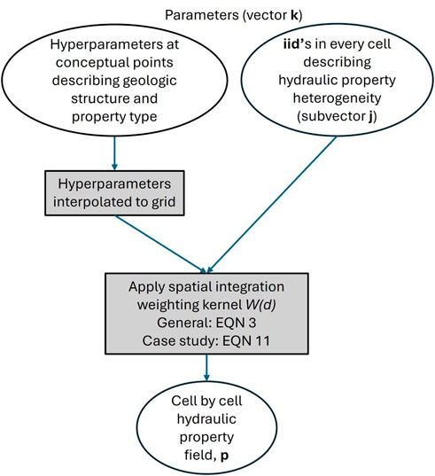
Figure 1. Workflow summary of the methodology used for generating hydraulic property fields with spatially varying anisotropy.

Where it is desired that W(d) hyperparameters exhibit spatial variability so that a model’s hydraulic property fields exhibit nonstationary stochastic behaviour, geostatistical hyperparameters can be ascribed to so-called “conceptual points”. These are broadly-spaced pilot points. Prior to populating the model grid with hydraulic properties, the values of these hyperparameters are spatially interpolated from conceptual points to the model grid. The W(d) function that is used in cell-by-cell hydraulic property assignment is therefore (a) specific to every model cell and (b) continuously variable in space.

2.3 Data space inversion

Data Space Inversion (DSI), creates a direct statistical relationship between the measured, historical behaviour of a system and aspects of its future behaviour that are of management interest. This relationship is formulated by sampling model outputs from an ensemble of model runs that employ random realizations of its parameters. Model outputs of interest correspond to field measurements on the one hand, and predictions of future system behaviour on the other hand. Observation-prediction relationships are then collated into a joint probability distribution. Once this joint probability distribution has been characterized, it can be conditioned by field measurements of actual system behaviour.

2.3.1 DSI strengths and weaknesses

One major advantage of DSI is that it does not require adjustment of numerical model parameters. Instead, parameters are sampled rather than adjusted, thereby avoiding the potential for model instability issues that can accompany parameter adjustment. A numerical model can therefore be endowed with hydraulic property fields of arbitrary complexity. This complexity can include categorical features such as faults and discrete alluvial channels whose existence, positions and properties may change from realization to realization.

Secondly, where model hydraulic property fields are generated using the weighted averaging technique that is described in the previous subsection, geostatistical hyperparameters can be sampled at the same time as iid parameters. Uncertainties in prior parameter uncertainties can therefore be taken into account when assessing the posterior (i.e., conditional) uncertainties of predictions of management interest. Without the need to resort to a sequential approach.

Third, the numerical burden of DSI-based predictive uncertainty analysis is very small compared to that of methodologies that require that parameter uncertainty be quantified as a precursor to quantification of predictive uncertainty. Conditioning of the DSI statistical model is numerically very fast. Meanwhile, only a few hundred samples of the joint past-future probability distribution are generally sufficient to characterize this distribution before conditioning it. The numerical simulator must therefore be run only as many times as is required to obtain these past-future samples.

Fourth, based on the premise that the worth of data increases with their ability to reduce the uncertainties of management-salient predictions, DSI can offer a rapid means of appraising the worth of existing or yet-to-be-acquired data; see, for example, He et al. (2018) and Delottier et al. (2023). DSI-based methodologies of data worth assessment have greater integrity than older methods such as those described by James et al. (2009), Dausman et al. (2010) and Wallis et al. (2014) that require an assumption of local model linearity.

Fifth (and finally), relationships between historical measurements and predictions of management interest are often less nonlinear than are those between measurements and model parameters. This can result in DSI-evaluated posterior predictive means and variances that are more reliable than those obtained by other means.

Naturally, potential advantages are accompanied by potential disadvantages. The theory on which DSI rests is based on an assumed Gaussian relationship between the measured past and the managed future. Histogram transformation of numerical model outputs that are used in this process can bestow Gaussian behaviour on individual model outputs (Sun and Durlofsky, 2017). However this does not guarantee Gaussianality of the joint measurement/prediction probability distribution as a whole. This inadequacy is partly overcome through construction of a parameterizable statistical model that encapsulates the joint past-future probability distribution. This statistical model is then subjected to iterative Bayesian history-matching; see below. Despite this, the performance of DSI can still suffer if past-to-future relationships are highly nonlinear. However, this potential problem must be seen in context. Similar considerations apply to all data assimilation methodologies, especially those that operate in high dimensional parameter spaces. Nevertheless, where predictions are likely to be discontinuous with respect to hydraulic properties and/or exhibit non-monotonic relationships with observations of past system behaviour, a modeller should use DSI (and all other data assimilation methodologies) with caution.

DSI is vulnerable to prior-data conflict. If it exists, prior-data conflict is readily exposed by undertaking model runs based on stochastic samples of the prior parameter probability distribution, a process that is integral to DSI deployment. Where stochastic model outputs that correspond to field measurements do not collectively span these measurements, then these measurements cannot condition the DSI statistical model. Where this occurs, a modeller should review his/her prior parameter probability distribution. Alternatively, a modeller may exclude offending measurements from the conditioning dataset on the basis that they reflect some aspect of system behaviour that the model is unable to replicate. This exclusion decision must be based on the premise that failure to replicate these nuances of past system behaviour does not invalidate the model’s ability to replicate those aspects of its future behaviour that are of management interest. We note that decisions of this kind must be made when implementing data assimilation by any means; DSI’s ability to assess the existence (or otherwise) of prior data conflict as part of its normal workflow can therefore also be seen as a strength.

Finally, where collections of model predictions exhibit consistencies in temporal or spatial behaviour that arise from the nature of these predictions (for example, monotonicity of a contaminant breakthrough curve), it is sometimes found that DSI predictions do not exhibit this same consistency. This is especially the case where a measurement dataset hosts little information that is pertinent to a particular prediction. While this may not detract from DSI estimates of posterior predictive mean and standard deviation, the optics are not good. In some instances this problem can be ameliorated by implementing a reduced dimensional representation of model outputs using, for example, basis functions that emerge from principal component analysis. Some authors have achieved reasonable success in overcoming this problem by combining DSI with other machine learning methodologies. See Jiang et al. (2021) and references cited therein for further details.

2.3.2 DSI mathematical details

An ensemble of parameter realizations k generated from the prior parameter probability distribution is run through a numerical model to produce an ensemble of model equivalent observations o and predictions s. Individual elements of these model output vectors are then (optionally) subjected to histogram transformation; we retain the symbols o and s to represent these transformed vectors. Using standard statistical analysis, empirical means of these vectors (i.e., ŝ and ô) are then obtained; along with the empirical covariance matrix of these vectors, which we represent below partitioned into its component submatrices.

${\mathrm{C}}_e\left(\left[\begin{array}{c}\mathbf{s}\\ \mathbf{o}\end{array}\right]\right)=\left[\begin{array}{cc}{\mathrm{C}}_{\text{ss}}& {\mathrm{C}}_{\text{so}}\\ {\mathrm{C}}_{\text{os}}& {\mathrm{C}}_{\text{oo}}\end{array}\right](5)$

This empirical covariance matrix is now subjected to singular value decomposition (SVD) in order to obtain matrices V and S that are defined by the following equation.

${\mathrm{C}}_e\left(\left[\begin{array}{c}\mathbf{s}\\ \mathbf{o}\end{array}\right]\right)=\mathbf{V}\mathbf{S}{\mathbf{V}}^{\mathbf{T}}(6)$

V is an orthonormal matrix while S is diagonal. Values of S decrease down its diagonal. The square root of the empirical covariance matrix is now calculated as:

${\mathrm{C}}_e^{½}\left(\left[\begin{array}{c}\mathbf{s}\\ \mathbf{o}\end{array}\right]\right)=\mathbf{V}{\mathbf{S}}^{½}{\mathbf{V}}^{\mathbf{T}}(7)$

Now consider the following “model” whose random parameters are encapsulated in a vector x whose mean is 0 and whose prior covariance matrix is the identity matrix I.

$\left[\begin{array}{c}\mathbf{s}\\ \mathbf{o}\end{array}\right]={\mathrm{C}}_e^{½}\left(\left[\begin{array}{c}\mathbf{s}\\ \mathbf{o}\end{array}\right]\right)\mathbf{x}+\left[\begin{array}{c}\underset{^}{\mathbf{s}}\\ \underset{^}{\mathbf{o}}\end{array}\right](8)$

Run time for the “model” of Equation 8 is of the order of hundredths of a second.

Using standard formulae for propagation of variance, it is easily established that if the model of Equation 8 is equipped with random samples of x, values of $\left[\begin{array}{c}\mathbf{s}\\ \mathbf{o}\end{array}\right]$ that are calculated using these samples possess the same mean and covariance matrix as those produced by the simulator using random samples of its parameters k. That is, the mean of $\left[\begin{array}{c}\mathbf{s}\\ \mathbf{o}\end{array}\right]$ calculated using Equation 8 is $\left[\begin{array}{c}\widehat{\mathbf{s}}\\ \widehat{\mathbf{o}}\end{array}\right]$, while the covariance matrix of $\left[\begin{array}{c}\mathbf{s}\\ \mathbf{o}\end{array}\right]$ calculated using Equation 8 is ${\mathrm{C}}_e\left(\left[\begin{array}{c}\mathbf{s}\\ \mathbf{o}\end{array}\right]\right).$

It follows that by sampling x which is easily done because each element of x is an iid, (not to be confused with the iid’s in subvector j in Equation 4), samples of the prior probability distribution of s can be obtained very quickly. What is more significant is that samples of the posterior probability distribution of s can be calculated from samples of the posterior probability distribution of x. The latter can be obtained by history-matching the model of Equation 8 against field measurements h corresponding to model outputs o, while adjusting the values of x. Bayesian history matching is easily implemented using methods such as Markov chain Monte Carlo, or an ensemble smoother. The latter option was adopted by Lima et al. (2020). The PEST suite (Doherty, 2024a) enables regularized calibration of the model of Equation 8 followed by fast calculation of posterior predictive confidence intervals in Gaussian space using a linearized formulation of Bayes equation (which is applicable in this space). Confidence intervals calculated in this way are then back-transformed to the space of native variables. The latter option is extremely fast. Experience shows that it also preserves temporal and spatial continuity relationships that are expected in numerical model outputs (see above). Figure 2 provides a summary of the workflow used to implement the DSI workflow.

Figure 2

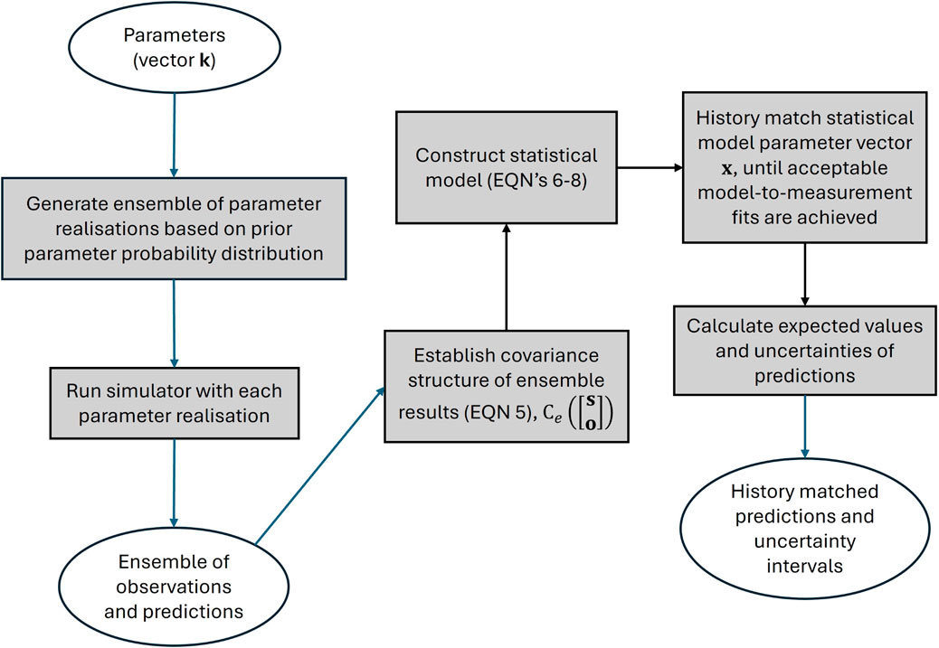
Figure 2. Workflow summary of the DSI methodology.

2.4 Ensemble space inversion

Although the principal foci of this paper are nonstationary stochastic field generation and DSI-based data assimilation, we provide a short description of ensemble space inversion (ENSI) as we use it in the case study (Section 3), to verify posterior predictive means calculated by DSI. ENSI is a numerically efficient and effective tool for model history-matching and is therefore worthy of deployment in many modelling contexts, either as a complement to other methodologies, or on its own.

2.4.1 ENSI strengths and weaknesses

We begin our description of ENSI by noting that, at the time of writing, the Iterative Ensemble Smoother (IES) is gaining increasing use in groundwater model history-matching. See Chen and Oliver (2012), White (2018) and PEST++ Development Team (2024) for a description of its algorithmic base and implementation details. Kalman ensemble methods have two strong attractions. The first is that they implement a numerical approximation to Bayes theorem, thereby sampling an approximation to the posterior parameter probability distribution. The second is that they can offer substantial computational savings by working in a reduced dimensional parameter subspace. The number of model runs required per iteration of a nonlinear data assimilation process is commensurate with the size of this subspace.

However, like all methods, strengths come with weaknesses. The Bayesian credentials of IES are challenged by model nonlinearity. Hence the calculated posterior may not be the true posterior, and an IES-calculated posterior predictive mean may suffer some bias (Evensen et al., 2022). At the same time, its confinement to a relatively low dimensional parameter subspace can sometimes limit the ability of IES to fit field measurements well.

Like IES, ENSI gains numerical benefits from dimensional reduction. Like IES, the parameter subspace in which ENSI works is defined by random samples of the prior parameter probability distribution. However, ENSI provides some flexibility in definition of this subspace by defining different subspaces for different parameter types. Parameter type subspaces can be of different dimensions; furthermore, factors by which different parameter realizations within a subspace are multiplied in order to form a history-match-conforming parameter set can be different for different subspaces. Different sets of parameters can therefore respond to information that is hosted by a history-matching dataset in ways that are best suited to them. This can elevate history-matching performance while mitigating parameter and predictive bias.

In addition to parameter realizations, ENSI also allows user-specified parameters to be adjusted on an individual basis as in traditional history-matching. This can be useful where a model is endowed with hierarchical parameterization; geostatistical hyperparameters are obvious candidates for individual, rather than collective, adjustment. Non-realization parameters such as these can therefore gain immunity from spurious adjustment as they are not realization-tethered to other parameters that may respond in different ways to information that is hosted by a calibration dataset. They are therefore free to respond to information within a calibration dataset in their own way without compromising passage of information to other parameters.

Unlike IES, ENSI does not sample the posterior parameter probability distribution. Instead, it seeks a unique, Tikhonov-regularized solution to an inverse problem. Ideally, this solution enables a model to make minimum-error-variance predictions of future system behaviour; generally these are close to the posterior means of their respective posterior probability distributions. In pursuing its solution to an inverse problem, ENSI calculates a Jacobian (i.e., sensitivity) matrix that links calibration-pertinent model outputs to realization factors and individual calibration-adjustable parameters. History-matching performance in the face of inverse problem nonlinearity can be improved through regular Broyden updating of this matrix. See Doherty (2024a) for details.

2.4.2 ENSI mathematical details

For a brief mathematical depiction of how ENSI works, we first divide the full parameter vector k of Equations 1 and 2 into multiple subsets. We denote the subset of parameters that are assigned to realization group i as k_i. Meanwhile, group-independent parameters are collectively denoted as k₀. The overall parameter vector k can therefore be written as follows, where n is the total number of realization groupings:

$\mathbf{k}=\left[\begin{array}{c}{\mathbf{k}}_0\\ {\mathbf{k}}_1\\ \dots \\ {\mathbf{k}}_n\end{array}\right](9)$

Suppose now that M_i random realizations of native model parameters that belong to realization group i are generated; the number of elements of k_i (we denote this as m_i), is generally considerably larger than M_i. Where a hierarchical parameterization scheme is adopted, the elements of k_i may be iid’s, so that the prior covariance matrix associated with this set of parameters is the m_i × m_i identity matrix. (Note that ENSI does not insist on hierarchical parameterization; so it is possible that each subset of parameters may be associated with an arbitrary covariance matrix.) Let the M_i realizations of k_i parameters comprise columns of the m_i × M_i matrix K_i. Let factors by which these realizations are multiplied be assigned to the M_i - dimensional vector f_i. Then elements of f_i are adjustable parameters in the re-formulated inverse problem.

A parameter set k that is used by a numerical model is computed from calibration-adjustable factor parameters that are manipulated by ENSI in the following way.

$\mathbf{k}=\left[\begin{array}{cccc}\mathbf{I}& \mathbf{0}& \dots & \mathbf{0}\\ \mathbf{0}& {\mathbf{K}}_1& \dots & \mathbf{0}\\ \dots & \dots & \dots & \mathbf{0}\\ \mathbf{0}& \mathbf{0}& \dots & {\mathbf{K}}_n\end{array}\right]\left[\begin{array}{c}{\mathbf{k}}_0\\ {\mathbf{f}}_1\\ \dots \\ {\mathbf{f}}_n\end{array}\right](10)$

Ideally, prior mean values of parameter types that are featured in different realization groups (for example, the prior mean value of all members of parameter group k_i) should be assigned to the nonrealization parameter group k₀. (This is not necessary for those iid parameters which correspond to the j vector in Equation 4, for their mean values should probably not be adjusted from zero.) Under these circumstances the preferred value of all realization factor parameters is 0. This is implemented as a Tikhonov regularization constraint. Meanwhile, the prior standard deviation of each element of the f_i parameter group is $\sqrt{M_i-1}$ (Iglesias et al., 2013; Chada et al., 2018). This is used to weight Tikhonov regularization constraints.

The workflow used to implement the ENSI methodology is summarised in Figure 3.

Figure 3

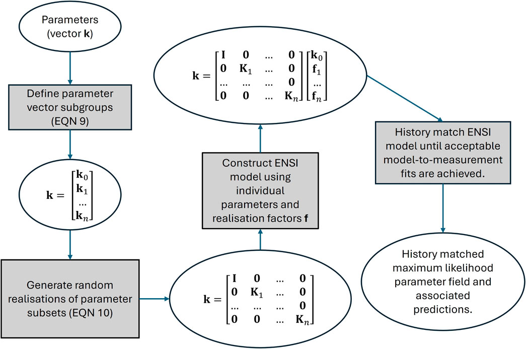
Figure 3. Workflow summary of the ENSI methodology.

The numerical cost of implementing ENSI is commensurate with that of IES as the number of parameter realizations that is required for effective implementation of these two processes is similar. Experience to date suggests, however, that ENSI is often able to attain a better fit with a history-matching dataset in fewer iterations than IES. Implementation of Broyden Jacobian updating appears to contribute significantly to its history-matching alacrity.

Based on this short comparison between ENSI and IES, it should not be construed that the authors of this paper see one as “superior” to the other. The authors view them as complementary to each other. Their principles of operation, and the numerical cost of their deployment, are somewhat similar. However, IES adjusts all realizations that comprise an ensemble while ENSI combines ensembles to attain a single parameter field that is, ideally, close to the posterior mean parameter field. For reasons described above, formulation of the ENSI inverse problem protects this field, to some extent at least, from estimation bias.

2.5 Summary

Three novel methodologies have now been described that, when used together or on their own, can improve the efficacy of decision-support groundwater model deployment in hydrogeologically heterogeneous environments.

Nonstationary stochastic field generation allows a modeller to construct adjustable parameter fields that encapsulate variable connectedness of hydraulic properties in different parts of a model domain. The locations of hydraulic property heterogeneity are represented by a dense spatial array of iid parameters, while heterogeneity patterns are governed by spatially variable geostatistical hyperparameters. These two sets of parameters (iid’s and hyperparameters) are independently adjustable.

In conjunction with a numerical model, DSI can use hydraulic property fields such as these to construct a statistical model that links field measurements of system behaviour to predictions of management interest. Once this statistical model has been built, it can be quickly conditioned using actual field measurements, thereby reducing predictive uncertainties. The numerical cost of the DSI process is limited to a few hundred simulations based on stochastic hydraulic property fields. The DSI process can readily accommodate both nonstationarity and uncertainty of geostatistical hyperparameters. Moreover, because model hydraulic property fields do not undergo adjustment, DSI can accommodate categorical expressions of hydraulic property heterogeneity.

ENSI achieves efficiencies in model calibration by working in a subspace of parameter space that is defined by realizations of a prior parameter probability distribution for different parameter types. This can lift history-matching performance while mitigating parameter bias in complex history matching contexts. The ENSI inversion algorithm appears to be robust in the face of nonlinearities induced by hierarchical inversion. Because parameters require adjustment, its model run burden is greater than that of DSI; it is of the same order as other dimension reduction methods such as IES.

3 A case study

3.1 General

This section describes groundwater issues, and a groundwater model, to which the methodologies that are described in the previous section are applied. The study area is in Aotearoa/New Zealand. The issue is potential risk to groundwater quality; however, the present study actually focusses on groundwater age, as young groundwater may contain pathogens that are introduced from agricultural and other activities through free draining soils that are then transported large distances through highly permeable aquifers. As a direct outcome of microbial decay, groundwater whose residence time is less than 1 year poses a greater risk to human health than groundwater that is older than this. There is a heightened awareness of this issue in New Zealand as microbial groundwater contamination has led to deaths in the recent past; see Gilpin et al. (2020). Groundwater in the study area is also contaminated by nitrates. While threats to human health posed by nitrates are not directly related to groundwater age, groundwater residence time impacts an aquifer’s response to changes in agricultural practice that may be implemented to address this issue.

3.2 Hydrogeology

The Wairau Aquifer, underlying the Wairau Plain, is situated in the northern part of the South Island of New Zealand; see Figure 4. With an area of approximately 360 km², this is the country’s largest wine-growing region. The Wairau River flows near the northern boundary of the Wairau Plain.

Figure 4

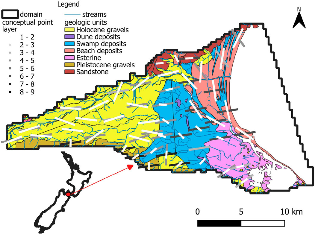
Figure 4. Overview of study area showing model domain, geology, stream network, and conceptual points used for depiction of spatially variable anisotropy of hydraulic property correlation. The orientation and length of each line indicates the direction and length of maximum spatial correlation (see Table 1). The darkness of these lines indicates the model layers to which respective conceptual points pertain. Specifiers such as 1+ indicate all layers from layer 1 to layer 13. The grey line indicates the approximate location of the transition from confined (west) to unconfined (east) conditions.

Table 1

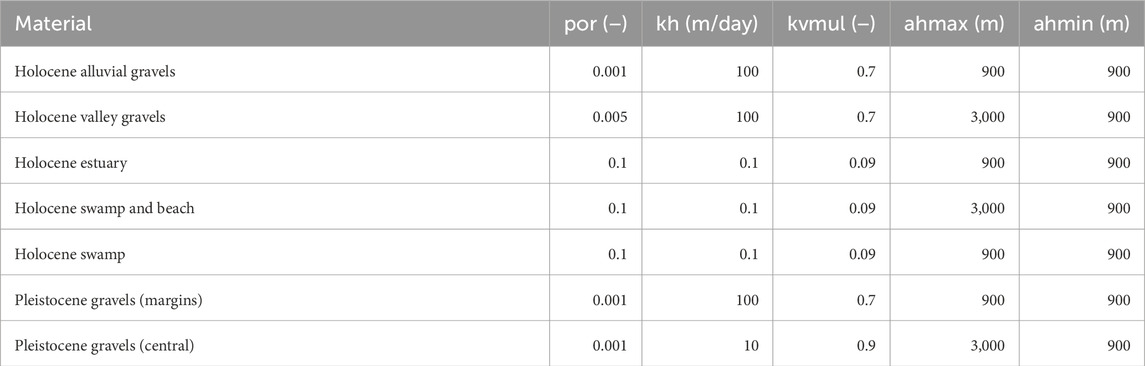
Table 1. Initial values of conceptual point hyperparameters. Standard deviations for all hyperparameters listed above are 2 orders of magnitude, i.e., (+/−) 2 in log10 space.

Glacial outwash sediments underlie the western part of the Wairau Plain (Holocene Rapaura Formation) while finer marine, estuarine, lagoonal, and aeolian deposits prevail in the east (Holocene Dillons Point Formation). The Holocene surficial gravels of the Rapaura Formation increase in thickness from approximately 10 m to approximately 20 m from west to east, with transmissivities varying between 1,000 and 4,000 m²/day. To the east, the finer deposits of the Dillons Point Formation extend to a depth of about 30 m, with lower transmissivities of up to 50 m²/day. A series of springs occur along the transition zone between the Rapaura and Dillons Point Formations. It is relevant to the following discussion that estimates of groundwater residence time for some of these spring waters are as low as a single year.

Both of these surficial Holocene formations overly glacial outwash deposits of Pleistocene age. These deposits are at least 80 m thick, with estimated transmissivities of 35 m²/day to 300 m²/day. In the eastern part of the Wairau Plains, groundwater flow can be confined. For further details of the hydrogeology of the Wairau Plains, see Davidson and Wilson (2011).

Pumping tests, lithological and geophysical logs, outcrops, and a consideration of depositional mechanisms suggest that hydraulic property heterogeneity is high throughout the alluvial gravel and glacial outwash sequences. Furthermore, spatial correlation of elevated and subdued hydraulic conductivity is likely to be higher in the direction of historical river and glacial outwash flow (roughly from west to east) than perpendicular to this direction. To the extent that spatial correlation of hydraulic conductivity anisotropy prevails in the finer sediments of the Dillons Point Formation, it is expected to be parallel to historical shorelines (which are roughly parallel to the present-day shoreline). Correlation anisotropy such as this can have a profound effect on movement of solutes, as well as on groundwater age (Engdahl and Weissmann, 2010; Moore et al., 2022).

Preferential pathways of open framework gravel permeate the alluvial and glacial outwash deposits (Ferreira et al., 2010). These are common to many New Zealand glacial outwash-alluvial reworked aquifers (Burbery et al., 2017). The impact of open framework gravels on overall aquifer transmissivity is generally mild, but their impact on contaminant residence time can be profound, for they comprise rapid transport pathways that have led to detection of pathogens at large distances from suspected pathogen sources (Gilpin et al., 2020). As will be discussed below, this has consequences for modelling of both contaminant movement and groundwater age in these aquifers. The small cross-sectional area of open framework gravels, combined with their extremely high permeability, requires the assignment of low effective porosities to their host formations in order for modelling to replicate high observed transport velocities (Dann et al., 2008; Thorpe et al., 1982; Tonkin and Taylor Ltd, 2018).

Initial estimates of aquifer properties such as hydraulic conductivity are based on Westerhoff et al. (2018). These estimates were used to support characterization of mean hydraulic properties. Meanwhile, estimates of hydraulic property spatial correlation lengths are informed by expert intuition. Together, these provide a probabilistic description of aquifer properties that can be embodied in the stochastic parameterization scheme of the numerical model. The reader is referred to relevant publications (White et al., 2016; Morgenstern et al., 2019; Raiber et al., 2012; Wöhling et al., 2018; Davidson and Wilson, 2011) and to Supplementary Material for more detail.

3.3 Water inflow

As discussed by Wöhling et al. (2018) and references cited therein, recharge to the Wairau Aquifer is dominated by the Wairau River, the Waihopa River (its dominant tributary), and other minor tributaries. Meanwhile, estimates of diffuse rainfall recharge are available from regional modelling that incorporates local climate, land use and soil type (Westerhoff et al., 2018). Recharge averages 145 mm/year over western alluvial Holocene material; however recharge is minimal under the fine coastal sediments that prevail in the eastern portion of the study area. Means and variances of recharge estimates are summarised in Supplementary Table S1.

The Wairau Aquifer also receives water from neighbouring groundwater systems through its boundaries with these systems. See Figure 5 below. Inflow rates vary considerably along the alluvial perimeter. They are estimated (with some uncertainty) on the basis of contributing areas and estimated recharge rates. Because of their uncertainties (and hence the need for their stochastic and adjustable representation), lateral inflow rates are declared as parameters in the Wairau model. See Supplementary Table S1 in the Supplementary Material for further details.

Figure 5

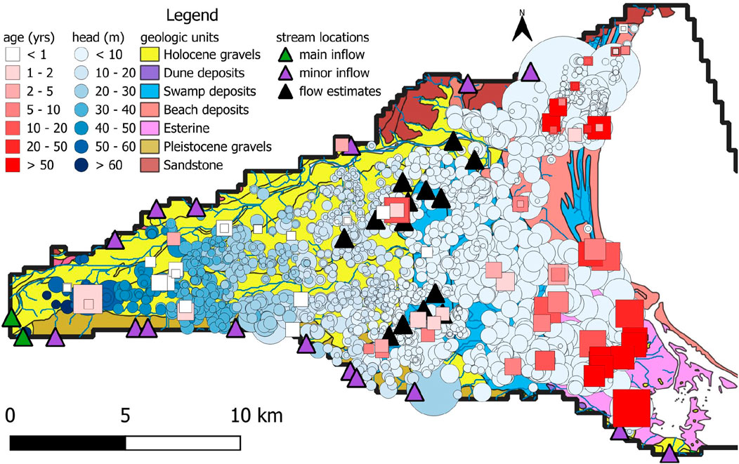
Figure 5. Locations of age/head history matching and stream inflow targets. Symbol sizes for age and head observations indicate observation depth in 10 m increments, with the smallest being less than 10 m and the deepest being greater than 100 m.

3.4 History matching observations

Estimates of long-term average water levels throughout the Wairau aquifer system at 1,778 locations are provided by White et al. (2016). Well screen intervals are generally shallower under the western portion of the aquifer than under its eastern portion, this reflecting the fact that deep permeabilities are higher than shallow permeabilities in the eastern part of the system; see Figure 4.

Estimates of mean flows in the Wairau River and 14 springs are also used for history matching (White et al., 2016, derived from Davidson and Wilson, 2011); see Figure 5.

Measurements of groundwater age have been made at 63 locations throughout the study area. (We use the terms “age” and “residence time” interchangeably in this paper.) Inferences of age vary between 1 day and 210 years (Figure 5). Most measurements were made in the eastern part of the study area where water is older. Increased water age in this area is an outcome of greater distance from recharge sources and slower rates of groundwater flow through coastal sediments.

3.5 Purpose of modelling

The primary purpose of modelling that is described herein is production of a three-dimensional map of groundwater age. Modelling therefore needs to reproduce age measurements that are depicted in Figure 5 while interpolating between these measurements in three dimensions. Of particular interest are low residence times, especially where these residence times are less than about a year. Unfortunately, as is apparent from Figure 5, most measurements of groundwater age were made in the eastern part of the study area where water is older, and hence poses less threat to human health. Only a few measurements have been made in western parts of the aquifer system where it is supposed that water is younger, and hence may pose a health risk.

Ideally, because groundwater age interpolation is simulation-based, and because measurements of heads and streamflows provide additional history-matching constraints, model-based age interpolation should have greater integrity than spatial interpolation that is undertaken in any other way. Nevertheless, local uncertainties are likely to be high. In recognition of this, modelling is tasked with quantifying these uncertainties. In doing so, it is also tasked with identifying locations where the likelihood of encountering young water is not vanishingly small.

4 Model construction and parameterization with spatially varying anisotropy

4.1 General

Numerical simulation of the Wairau Aquifer is now described. For brevity, we only include details of the modelling process that are pertinent to the theme of this paper.

4.2 Numerical model structure and design

Groundwater flow is simulated using MODFLOW 6 (Langevin et al., 2017). The model grid is structured and laterally uniform. All cells are square with a side length of 300 m. The model grid is shown in Figures 6A,B.

Figure 6

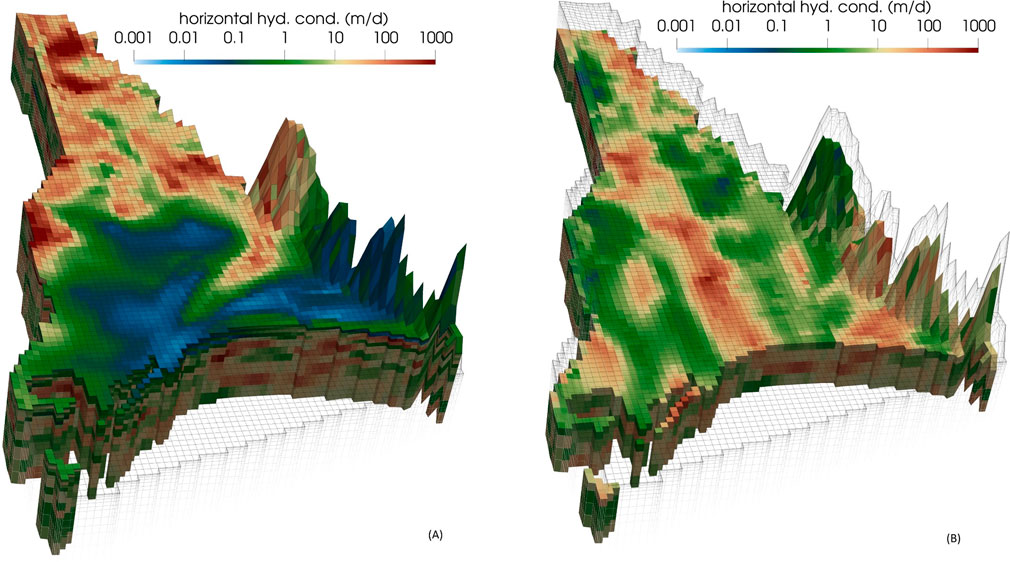
Figure 6. Random realization of horizontal hydraulic conductivity for (A) layer 1 and (B) layer 10 of the Wairau model.

In order to represent variation of hydraulic properties with depth, and in order to support simulation of three-dimensional travel paths of water and contaminants through material with depth-dependent hydraulic properties, the model possesses 13 layers. Layer thicknesses are uniformly 1, 2, 4, 6, 8, 10, 10, 20, 20, 20, 33, 33 and 33 m. Hydraulic properties that are representative of Holocene gravels extend to the base of layer 5, while those that represent finer coastal Holocene sediments extend to the base of layer 6. These overly layers that represent Pleistocene glacial outwash deposits.

The model simulates steady state flow. Groundwater interaction with the sea is represented using a general head boundary (i.e., GHB). This is located in model layer 1; it extends seaward from the coast for about 2 km.

Water enters the model vertically through recharge (simulated using the RCH package) and laterally through small amounts of inflow (i.e., “mountain front recharge”) through its northern, southern and western boundaries (simulated using the WEL package). As discussed above, these lateral inflows are calculated from estimated recharge rates and areas of upgradient, contributing catchments.

The streamflow routing package (SFR, Niswonger and Prudic, 2005) is used to simulate flow in the Wairau River and its tributaries. SFR reaches are assigned to cells that include streamlines that are depicted in Figure 5. Upstream inflows into the Wairau and other rivers are estimated from pertinent stream gauging data (where available); these are declared as parameters so that they are adjustable. SFR conductances are calculated from layer 1 vertical hydraulic conductivities, observed and estimated stream widths, and intersection lengths of mapped streams with model cells. Spatially distributed multiplier parameters are applied to these stream conductances in order to support history-match adjustment.

Ubiquitous high-conductance, surface-emplaced drain cells (simulated using the DRN package) are connected to the MODFLOW 6 water mover (MVR) package. These conduct surface water seepage to the nearest SFR stream reach.

Groundwater age is calculated by particle backtracking using MODPATH 7 (Pollock, 2016). Five hundred particles are emplaced on a cylinder of radius 1 m and height 2 m surrounding each subsurface age measurement point. The model calculates groundwater age as the average travel time of these 500 backtracked particles. For predicting age at cells without age measurements (these being model predictions of interest), a single particle is placed at the centre of each cell and backtracked to its recharge source. In both cases, particles that emerge at mountain front recharge boundaries are ascribed a history-match-adjustable age increment that increases with depth of exit. A spatially-variable increment-versus-depth function is ascribed to all laterally emergent particles.

The model run time is generally 5–10 min, this including parameter preprocessing and model output postprocessing. However, this can extend to 30 min for some parameter sets.

4.3 Conceptual point hyperparameters

As discussed above, spatially-varying, layer-specific hyperparameters that embody geostatistical descriptors of hydraulic property variability are ascribed to conceptual points. One suite of hyperparameters is required for horizontal hydraulic conductivity (kh), another suite is required for the ratio of vertical to horizontal hydraulic conductivity (kvmul), and another suite is required for porosity (por). Five hyperparameters are ascribed to each conceptual point for each of these three hydraulic property types. These are as follows:

• mean value;

• variance (i.e., sill);

• bearing of major axis of correlation anisotropy;

• length of major axis of correlation anisotropy (ahmax) (i.e., correlation length in the dominant direction of anisotropy);

• length of minor axis of correlation anisotropy (ahmin) (i.e., correlation length in the minor direction of anisotropy).

In the modelling workflow described herein, only some of these hyperparameters are varied in order to express uncertainty and respond to history-matching; see below. The remaining hyperparameters are fixed at user-prescribed values.

The length of an axis of anisotropy (ahmax or ahmin) is the value of a that appears in the following depiction of the Gaussian function; d represents distance. This function is employed by the spatial integration kernel which transforms cell-based iids to spatially correlated, cell-based hydraulic properties.

$f\left(d\right)=e^{-{\left(\frac{d}{a}\right)}^2}(11)$

48 conceptual points are assigned to each model layer. Conceptual points have the same x and y coordinates in all of these layers. Interpolation of geostatistical hyperparameters from conceptual points to cells of the model grid is implemented using two-dimensional kriging that is based on spatially varying variograms that reflect local anisotropy. See Doherty (2024c).

Figure 4 shows the locations of conceptual points together with associated ahmax lengths and directions. These are overlain on a geological map of the study area. Assignment of values to conceptual-point-hosted hyperparameters reflects local geologic structure and hydraulic property type. See Table 1. Note that ahmax, ahmin and orientation parameters are fixed (i.e., are nonadjustable) in the present study.

Immediately noticeable from Table 1 are the low values of prior mean porosity. (Recall that porosity is parameterized; hence values of porosity throughout the model domain are history-match-adjustable.) As discussed above, prior porosity values reflect experience in history-matching other New Zealand models with similar geology. They reflect the presence of preferential pathways comprised of highly permeable open framework gravels whose connected cross-sectional areas are considerably smaller than that of numerical model cells. Use of low prior porosities in this context can therefore be considered as an upscaling strategy, or a property of the medium that prevails at a representative elementary volume that is roughly the size of a model cell (Kenny et al., 2025; Dann et al., 2008). As such, its use embodies similar concepts to that of dual porosity in which a medium is declared to possess coincident mobile and immobile flow domains. Preferential pathways are likely to have little effect on bulk hydraulic conductivities, but are able to transport solutes (and possibly viruses) large distances in short times (Thorpe et al., 1982; Dann et al., 2008; Tonkin and Taylor Ltd, 2018).

4.4 Model parameterization

4.4.1 General

The Wairau Aquifer model possesses 51,714 active model cells. Three groups of iid parameters are assigned to each of these cells, one for the log of porosity (por), one for the log of hydraulic conductivity (kh), and one for the log of the ratio of vertical to horizontal hydraulic conductivity (kvmul). These iids are spatially integrated to obtain values of the logs of pertinent hydraulic properties at model cells. The integration function is specific to each model cell. It reflects local values of cell-interpolated hyperparameters that are depicted in Table 1. Generation of random values for iids is straightforward as they are normally distributed and independent of each other. The total number of iid parameters is 155,142.

Hyperparameters comprising mean values for por, kh and kvmul are ascribed to each of the 624 conceptual points, this resulting in 1,872 hyperparameters that are history-match-adjustable. Spatial correlation between these hyperparameters is presumed to be horizontal and spatially variable, with ahmax and ahmin values equivalent to those ascribed to the conceptual points themselves. Covariance matrices that embody this assumption are used for generation of random values of these hyperparameters. All other conceptual point hyperparameter values are declared as fixed.

A spatially-correlated addend field is applied to recharge. Recall that steady state recharge rates are calculated by a regional recharge model that takes local climate, soil type and land use into account. In order to introduce the possibility of additional spatial variability beyond that provided by the regional recharge model, the recharge addend field is interpolated from 121 pilot points that are distributed over a regular grid that spans the model domain. The addend field is characterized by a mean value of 0.0 and a covariance matrix with a variance of 10^–6 (m/day)² and a spatial correlation length of 9 km (see Supplementary Table S1).

Other parameters used by the Wairau model are as follows:

• stream stage above stream bed;

• stream conductance multipliers;

• rate of groundwater age increase with depth at lateral model boundaries;

• multipliers applied to lateral boundary inflow rates;

• GHB conductances at the seaward model boundary;

• boundary inflows into stream segments.

All but the last of these parameters are spatially distributed. Prior means, variances and correlation lengths are provided in Supplementary Material.

Altogether, the Wairau Aquifer model is endowed with 163,359 parameters. Collectively, they reflect what is known about the Wairau groundwater system (through their prior probability distributions) and what remains unknown about the system (through the range of values that are compatible with these distributions).

4.4.2 Model parameterisation and DSI

Five hundred runs of the Wairau numerical model were devoted to training of the DSI statistical model. On each occasion that it was run, the numerical model was equipped with a single realization of all model parameters (including hyperparameters) that are described in previous paragraphs. For each model run, model outputs that complement field measurements, together with model predictions of management interest, were recorded. These were subsequently used to construct the empirical covariance matrix of Equation 5. In the present case, predictions of interest comprise groundwater ages calculated for every model cell.

4.4.3 Model parameterization and ENSI

As for DSI, implementation of ENSI requires generation of random parameter fields. ENSI combines these fields to produce a single, regularized hydraulic property field. As discussed above, separate combinatorial factors can be applied to realization groups that are comprised of different parameter types. So, prior to implementing ENSI, a modeller must separate parameters into different realization groups. He/she must then assign a certain number of realizations to each of these groups. As discussed above, individual parameters can also be estimated.

The number of realizations assigned to each realization group for the study that is documented herein is listed in Table 2.

Table 2

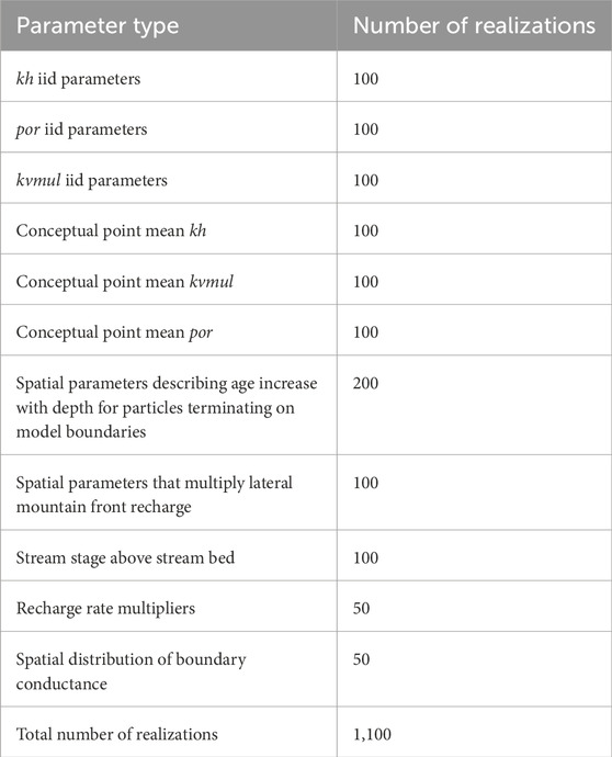
Table 2. Number of realizations assigned to different parameter groups.

The ENSI parameter set also includes 18 non-realization parameters. These are inflows to SFR stream segments along the model boundary.

4.5 Example realizations

Figure 6 shows a single realisation of hydraulic conductivity for layers 1 and 10 of the model. Note how, in the upper of these two model layers (which represents Holocene deposits), high values of hydraulic conductivity in the western part of the model domain merge smoothly into low values of hydraulic conductivity in the eastern part of the model domain as gravels grade into silts and clays. Note also how the patterns and orientations of hydraulic conductivity change shape and direction when moving from west to east.

In contrast, the geostatistical properties of Pleistocene glacial outwash material that underlies the shallow Holocene deposits exhibit less spatial variability than the material which overlies it. Hence patterns of heterogeneity are the same in both the eastern and western parts of layer 10 of the model domain.

5 Data assimilation results

5.1 DSI

As stated above, the numerical model of the Wairau Aquifer was run 500 times in order to train the DSI statistical model. For each of these runs, the model was populated with a different stochastic parameter field. Measured heads, streamflows and log-transformed measured groundwater ages comprise the vector h (i.e., the history-matching dataset) of Equations 5–8, while model outputs corresponding to these measurements comprise the vector o. The vector s (i.e., the suite of model predictions) contains logs of groundwater age calculated for every cell of the model domain.

The DSI statistical model of Equation 8 has a run time of a fraction of a second as it requires only that a vector be multiplied by a matrix. This makes history-matching easy. History-matching options include those that would normally be considered for a numerical groundwater model, these including regularized inversion or ensemble smoothing. However, because of its short run time, options such as Markov chain Monte Carlo that would not normally be used for groundwater model history matching can also be considered. In all cases, the x parameters of Equation 8 are adjusted until a desired level of fit is attained between statistical model outputs and field measurements. Ideally, history-matching using regularized inversion yields groundwater log (age) predictions that approximate their posterior means. Alternatively, an ensemble smoother enables direct sampling of the posterior predictive probability distribution of log (age).

In the present study, we implement history-matching using regularized inversion. As is discussed in Section 2.3, statistical linkages embodied in Equation 8 are generally made after histogram transformation of observations and predictions to Gaussian space. Predictions made by the statistical model must then be back-transformed to the space of natural numbers. Software available through the PEST suite associates predictive confidence intervals with back-transformed, calibrated statistical model predictions without the need to sample posterior predictive probability distributions. This is done by first implementing linearized Bayes equation in Gaussian space (where it is applicable) and then back-transforming to the space of natural numbers. This approach to DSI model history-matching and uncertainty analysis has the advantage that it reduces the propensity for nonphysical DSI model output behaviour that is discussed in Section 2.3. See Doherty (2024a) for details. In the present study, however, implementation of histogram transformation was found to offer no advantage. So calculation of uncertainties in this manner was applied to untransformed model predictions.

Fits between DSI statistical model outputs and field measurements are summarized in Figure 7. Head misfits can be attributed to a number of causes. These include invalidity of the steady state assumption, and the effects of local nuances of hydraulic properties that cannot be represented using prior parameter and hyperparameter probability distributions that are employed in this study. Root mean square errors are 1.69 m for heads, 0.59 log₁₀ (m³s^-1) for streamflows and 0.07 log₁₀ (years) for groundwater age. The objective function that was used to define model-to-measurement misfit, and that was minimized during the DSI statistical model calibration process, used different weights for different observations of each type in order to reflect relative measurement credibilities. Following this philosophy, weights assigned to streamflows were such that they comprised about 10% of the total objective function because local channel characteristics, especially elevation, are represented only approximately at the scale of the model grid. (Note that the log scale used for streamflows in Figure 7, appears to exaggerate misfits with small flows.).

Figure 7

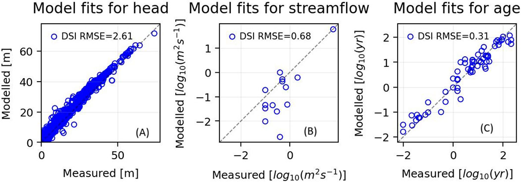
Figure 7. Model-to-measurement fits for (A) groundwater head (B) log(to base 10) of streamflow and (C) log(to base 10) of groundwater age.

A number of factors contribute to model misfit of groundwater age measurements. These include processes that determine groundwater residence time, as well as those that effect the groundwater age measurement process itself. Ideally, given the purpose of the current study, a model-calculated age should be matched against that of the youngest water in the vicinity of the age measurement point. However, because of local hydraulic property heterogeneity, it cannot be guaranteed that a particular measurement borehole has access to the youngest local water. Furthermore, extraction of water from a borehole is likely to mix locally younger water with locally older water. Some older water may therefore be withdrawn from material of low hydraulic conductivity that juxtaposes a measurement borehole that is screened in hydraulically conductive material.

Figure 8 depicts posterior mean groundwater age in layers 6 and 9 of the numerical model as calculated by the calibrated DSI statistical model. (These layers were selected for representation in this and ensuing pictures because they are representative of conditions in the upper and lower portions of the Wairau Aquifer. Their significance for vulnerability assessment is no different from that of other layers, however.) The predicted youthfulness of deep water in some parts of the model domain is readily apparent from this figure. By way of comparison, Figure 9 depicts ages in these same layers calculated using prior mean hydraulic properties. It is apparent that data assimilation reduces predicted groundwater age considerably in many parts of the Wairau Alluvium.

Figure 8

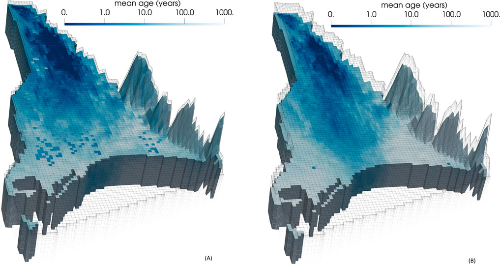
Figure 8. Posterior mean estimates of groundwater age in (A) layer 6 and (B) layer 9 of the model domain as calculated by the calibrated DSI statistical model. These correspond to depths of approximately 31 m and 61 m respectively.

Figure 9

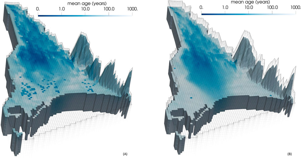
Figure 9. Prior mean estimates of groundwater age in (A) layer 6 and (B) layer 9 of the model domain.

The posterior standard deviation of uncertainty of predicted groundwater age in layers 6 and 9 is mapped in Figure 10, using a log(to base 10) scale. Uncertainties are high near the coast and relatively low in other parts of the model domain where groundwater age is predicted to be low.

Figure 10

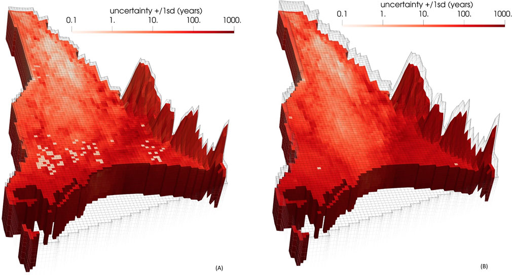
Figure 10. Posterior standard deviation of log(to base 10) of groundwater age in (A) layer 6 and (B) layer 9 of the model domain as calculated by the calibrated DSI statistical model.

Figure 11 shows the ratio of the posterior standard deviation of log age to the prior standard deviation of log age in these same layers. Lighter colours indicate low values of this ratio, and hence larger reductions of uncertainty accrued through history-matching; any value less than 1.0 indicates at least some reduction in the uncertainty of predicted groundwater age. The uncertainty-reducing effects of data assimilation are readily apparent. This is particularly significant near the Wairau River in the west of the study area where previous studies have shown high rates of groundwater recharge from the river (Davidson and Wilson, 2011; Wilson et al., 2023).

Figure 11

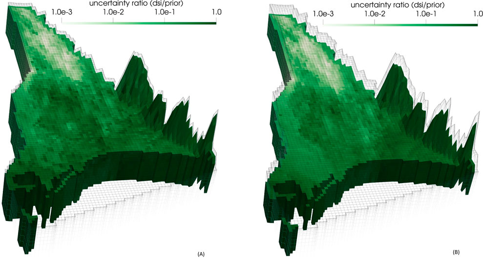
Figure 11. Ratio of posterior (DSI calibration) to prior standard deviation of log(to base 10) of groundwater age in (A) layer 6 and (B) layer 9 of the model domain.

Figure 12 illustrates how uncertainty analysis can assist groundwater management through its ability to associate risk with prognoses of future groundwater condition. The two parts of this figure (each pertaining to a different model layer) depict the 95% confidence limit of groundwater youthfulness. That is to say, there is only a 5% chance that groundwater is younger than values that are mapped in this figure, while there is a 95% chance that it is older. Areas where there is less than a 5% probability of water being younger than a single year are omitted from these figures.

Figure 12

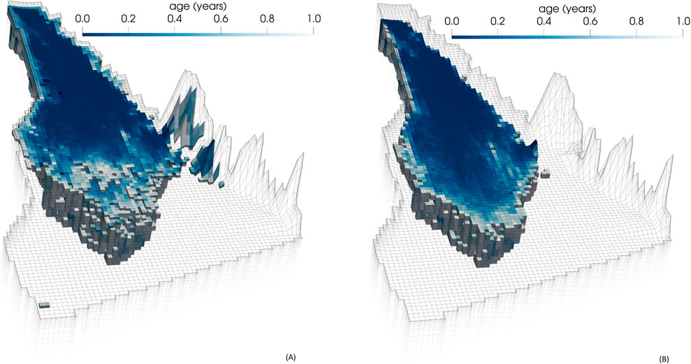
Figure 12. Groundwater age predictions corresponding to the 5% quantile in (A) layer 6 and (B) layer 9 of the model domain as calculated using the calibrated DSI statistical model.

Finally, we explore the comparative efficacy of head and streamflow data on the one hand, and groundwater age data on the other hand, in reducing uncertainties of regional groundwater age predictions. Figure 13 depicts improvements in uncertainty reduction accrued through joint use of age, head and streamflow measurements over that achieved through use of head and streamflow measurements alone. It does this through displaying the ratios of posterior uncertainties calculated on the basis of these two calibration datasets. Values of less than unity (lighter colours in Figure 13) imply lower predictive posteriors when history-matching is undertaken against age/head/streamflow data than when it is undertaken against head/streamflow data alone. It is apparent from these two figures that uncertainties in predicted groundwater age are generally much greater when these predictions are constrained only by head and streamflow measurements than when they are constrained by head, streamflow and age measurements. Other analyses demonstrate this in different ways. For example, a plot of posterior mean groundwater age calculated using a DSI statistical model that is calibrated against heads and streamflows alone (see Supplementary Figure S1) exhibits ages that are similar to those calculated using prior mean parameter fields.

Figure 13

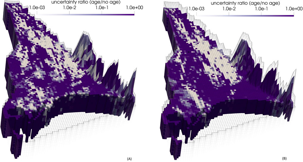
Figure 13. Ratio of posterior predicted age standard deviations with and without age measurements included in the DSI calibration dataset for (A) layer 6 and (B) layer 9 of the model. Lighter colours depict areas where historical measurements of groundwater age are most effective in reducing the uncertainties of future groundwater age predictions.

5.2 ENSI

Calibration of the numerical model of the Wairau Aquifer using ENSI attained an acceptable level of model-to-measurement misfit in 6,711 model runs. Nevertheless, the inversion process was allowed to continue until model-to-measurement misfit was minimized, thereby reducing the objective function by a further 5%; this required a total of 49,245 runs over 22 iterations of the regularized inversion process. Fits between model outputs and field measurements are commensurate with those attained through calibration of the DSI statistical model, and so are not presented as a separate figure. After 6,711 model runs, root mean square errors are 2.17 m for heads, 1.70 for streamflows and 0.42 log10 (years) for groundwater age.

ENSI-calibrated hydraulic conductivity fields for layers 6 and 9 are displayed in Figure 14. Unsurprisingly, these fields are smoother than samples of the prior hydraulic conductivity distribution that are displayed in Figure 6. This is an expected outcome of regularized inversion whose purpose is to find the “simplest” solution to an inverse problem while maintaining geostatistical correctness of that solution. See Doherty (2015) for further details.

Figure 14

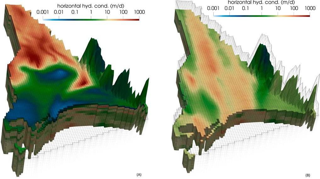
Figure 14. ENSI-calculated hydraulic conductivities in (A) layer 1 and (B) layer 9 of the model domain. These can be compared to selected prior realisations of hydraulic conductivity provided in Figure 6.

Groundwater age predictions made using the ENSI-calibrated model are shown in Figure 15. These are commensurate with predictions of groundwater age made using the calibrated DSI statistical model; see Figure 8. While qualitative agreement between predictions made using ENSI on the one hand, and DSI on the other hand (one method requiring adjustment of complex parameter fields and the other requiring adjustment of parameters used by a statistical model), does not constitute validation of either method, consistency of results lends credibility to both of them.

Figure 15

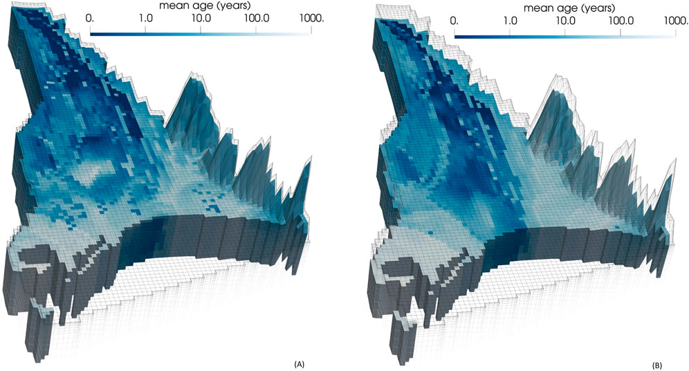
Figure 15. Predictions of groundwater age in (A) layer 6 and (B) layer 9 of the ENSI-calibrated model.

6 Discussion

6.1 Numerical implications

In this paper we present and demonstrate the utility of a methodology that enables generation of complex, stochastic, non-stationary hydraulic property fields. The hydraulic property parameters from which these hydraulic property fields are computed are Gaussian, continuous, and adjustable. Furthermore, hyperparameters that govern hydraulic property patterns can be simultaneously adjusted during history-matching. The case study demonstrates how these two parameter types can therefore express, in a semi-realistic manner, hydrogeological complexities on which model outputs may depend, and how they can respond to information related to locations and patterns of anomalous heterogeneity that may reside in a history-matching dataset. At the same time, this type of parameterization can readily express the consequences of information insufficiency for predictive uncertainty.

An advantage that accompanies the use of iid parameters to represent hydraulic properties is that they retain their geostatistical identity even as hyperparameters that dictate the spatially-variable correlation structure of groundwater system hydraulic property fields are adjusted during history-matching. This enables relatively easy implementation of hierarchical inversion. It also enables expression of uncertainties in prior hydraulic property uncertainty when building a DSI statistical model.

Advantages of DSI as a device for predictive uncertainty quantification and reduction that have been demonstrated through the case study include the following:

1. The numerical cost of DSI is small. It requires that only a few hundred runs of a numerical simulator be undertaken using samples of its prior parameter probability distribution. Data is assimilated using a fast-running surrogate statistical model, reducing the computational costs of history matching by orders of magnitude.

2. DSI can therefore be employed in conjunction with simulators whose run times are long, and whose numerical stability may not withstand the rigours of parameter-based data assimilation implemented through either ensemble-based history-matching or regularized inversion.

3. When implementing DSI, the prior probability distribution of hydraulic and other system properties can be represented using geostatistical descriptors of arbitrary complexity. Furthermore, they can include uncertainty in prior uncertainty, i.e., the uncertainties of values of geostatistical hyperparameters.

4. DSI analysis is easily extended to include appraisal of the comparative worth of different data and/or different data types.

The data worth analysis that is exemplified in the present study is simple, requiring only the omission of part of an existing history-matching dataset from the data assimilation process. However, with little extra effort, more complex analyses can explore the worth of data that has not yet been acquired. This can be achieved by comparing DSI-evaluated predictive uncertainties with and without the inclusion of model-generated “measurements” of system behaviour in a DSI history-matching dataset (Delottier et al., 2023). Appraisals of data worth that are undertaken in this manner can underpin design of data acquisition strategies that maximize returns on data investments.

Parameter-based data assimilation is required where information pertaining to the disposition of subsurface hydraulic properties is sought. However, where a complex, slow-running model is endowed with many parameters, and where data assimilation requires adjustment of all of these parameters, then history-matching must be implemented using a dimensional reduction scheme. ENSI provides flexibility in reducing the dimensionality of an inverse problem, and with it the number of model runs that is required for solution of that problem.

The case history that is described above demonstrates ENSI’s ability to subject different parameter types, as well as individual parameters, to history-match-adjudicated manipulation in their own subspaces without interference from other parameter types. Its use in hierarchical inversion has also been demonstrated.

A shortcoming of ENSI inversion is that it does not assess posterior parameter uncertainty. Uncertainty quantification must therefore be undertaken using other methods. However, in attaining a good fit with a measurement dataset, ENSI inversion provides a useful starting point for application of these methods. For example, random parameter samples that are used by an iterative ensemble smoother such as PESTPP-IES may be centred on an ENSI-calibrated parameter field. If this is done, the hard work of achieving a good fit with a measurement dataset, possibly under nonlinear circumstances that may challenge the performance of an ensemble smoother, has already been accomplished. Similarly, random parameter sets centred on an ENSI-calibrated parameter field can be used for DSI analysis. Another option is to undertake linear, first order second moment (FOSM) analysis following ENSI inversion using an ENSI-calculated Jacobian matrix.

6.2 Implications for groundwater management

DSI-predicted groundwater residence times that are pictured in Figures 8, 12 are smaller than those anticipated on the basis of system properties that are informed by expert knowledge alone; see Figure 9. In particular, they depict deep groundwater as being younger than expected. DSI-based uncertainty analysis exposes even more pessimistic possibilities; see Figure 12.

Implications for Wairau Aquifer groundwater management may be significant. This study suggests that continuous monitoring of aquifer-extracted drinking water for viral and other contaminants may be warranted. This is because contaminants have opportunities for rapid transport from their sources to drinking water extraction points. These opportunities are offered by alluvial sediments that include depositional features with highly connected permeabilities.

Of equal importance is the mechanism through which these opportunities for rapid advection have been exposed. The present study shows that information forthcoming from head and streamflow measurements does little to illuminate risks posed by fast advective transport of pathogens through a highly permeable and heterogeneous groundwater system. It appears that the best way to inform groundwater age is to calibrate a numerical model (or its statistical surrogate) against measurements of groundwater age, to the extent that these are available. Correspondingly, the best way to reduce uncertainties in groundwater age is to take more age measurements, especially at locations that are important to maintenance of human health.

Calculation of younger-than-expected groundwater residence times has some beneficial repercussions. It suggests that alterations to agricultural practices and land management that may require implementation in order to reduce the amount and location of nitrate pollution may achieve positive outcomes in a reasonably short time.

7 Conclusions

Protection and management of the health and sustainability of a groundwater system requires an ability to extract management-pertinent information from all available data. It also requires that the repercussions of information insufficiency be clearly presented to decision-makers so that they are aware of the risks that accompany any management strategy that they may pursue.

Three technologies which are new to groundwater modelling are presented in this paper. Whether used together or separately, these can enable those who provide technical support to groundwater managers to increase the value of that support. They are all designed to enhance the utility of numerical simulation as a groundwater management tool. In particular, they are all designed to increase the ability of numerical simulation to extract information from measurements of past system behaviour in order to express and reduce uncertainties in predictions of future system behaviour.

Adoption of numerical simulation as a means of information harvesting and delivery rests on the premise that unbiased predictions of management interest can be made, and that these predictions can be endowed with uncertainty intervals that are realistic, and that have been reduced to the extent that available information allows. Credibility of model-evaluated uncertainty intervals requires that model parameter fields express the proclivity for hydraulic property heterogeneity, and (just as importantly) the proclivity for hydraulic conductivity connectedness, that prevails in the subsurface. However, adjustment of realistic hydraulic property fields in order to constrain uncertainties through history-matching is a numerically demanding process. Methodologies that deliver most efficiency to this process generally make use of ensembles of model parameters, as these methodologies enable history-matching to take place in a subspace of parameter space that is far smaller than the dimensionality of parameter space itself. The latter must often be large in order to represent system complexities to which management-salient predictions may be sensitive.

In this paper we demonstrate how Ensemble Space Inversion (ENSI) can be deployed to adjust complex parameter fields (including those that embody nonstationary geostatistics) in order to fit a multi-component history-matching dataset comprised of groundwater head, streamflow and groundwater age measurements. Depending on the hydrogeological context, ENSI’s model run efficiency and history-matching alacrity is either commensurate with, or exceeds, that of other ensemble-based methods. Furthermore, ENSI is able to readily accommodate inversion nonlinearities incurred by the simultaneous adjustment of geostatistical hyperparameters and hydraulic property parameters (that is, hierarchical inversion).

In contrast to ENSI, Data Space Inversion (DSI) requires no parameter adjustment. Nor does it require that model-imbued hydraulic property fields be either stationary or adjustable. Furthermore, it can accommodate uncertainties in hyperparameters that describe the geostatistical properties of hydraulic property fields. The numerical burden of implementing DSI is generally only a few hundred model runs. These are generally sufficient to construct a statistical model that links measurements to predictions. Data assimilation is then conducted using the statistical model at minimal numerical cost.

Like other data assimilation methodologies and tools, those that are documented herein have their strengths and weaknesses. Hence there are advantages to be gained in using them in combination with other methods, and indeed with alternative methods of aquifer vulnerability assessment that do not rely on numerical simulation (if vulnerability assessment is the intention of their deployment). Their numerical efficiency, and their ability to quantify and reduce the uncertainties of management-salient predictions, should favour their adoption at many sites.

We finish this paper by noting that all of the methodologies that are described herein can be implemented using software from the PEST suite. At the time of writing, all but ENSI are presently available through the PEST++ and supporting PyEMU suites.

Terminology

Broyden updating: improvement of a Jacobian (i.e. sensitivity) matrix based on information acquired through testing parameter upgrades. Conceptual points: points in two-or three-dimensional space to which hyperparameters are assigned. Values of hyperparameters are spatially interpolated to cells of a model grid from these points. Covariance matrix: used to describe joint probabilities of multiple random variates. Diagonal elements of this matrix express variance (square of standard deviation)of individual variates. Off-diagonal elements express covariance between pairs of variates. Data assimilation: in general, this term refers to uncertainty reduction accrued through harvesting of information from data. In groundwater modelling, this is generally achieved through history matching. DSI: data space inversion. Ensemble: a collection of realizations drawn from a probability distribution. ENSI: ensemble space inversion. IES: iterative ensemble smoother. Hierarchical inversion: an inversion process in which parameters include hydraulic properties as well as hyperparameters which govern the prior probability distributions of hydraulic properties. Histogram transformation: a term borrowed from image processing that has been adopted by DSI literature. In the present context it is equivalent to normal score transformation. Hyperparameters: parameters employed by functions that characterize the prior probability distributions of parameters used by a model. Iid: independent and identically distributed random variable. Nonstationary: used to describe a context in which geostatistical hyperparameters vary in space. Pilot points: points in two- or three-dimensional space to which parameters are assigned. Hydraulic properties are assigned to cells of a model grid by spatial interpolation or weighted spatial averaging, depending on their mode of deployment.

Data availability statement

The original contributions presented in the study are included in the article/Supplementary Material, further inquiries can be directed to the corresponding author.

Author contributions

WK: Data curation, Formal Analysis, Investigation, Validation, Visualization, Writing – original draft, Writing – review and editing. CM: Conceptualization, Formal Analysis, Funding acquisition, Methodology, Project administration, Supervision, Writing – original draft, Writing – review and editing. JD: Formal Analysis, Methodology, Software, Writing – review and editing.

Funding

The author(s) declare that financial support was received for the research and/or publication of this article. This work was funded by the New Zealand Ministry of Business Innovation and Employment (Grant No. C05X1803) and was also supported by GNS Science Groundwater Strategic Science Investment Fund (SSIF). Funding from GMDSI for the development of some of the software and methodologies discussed herein is acknowledged and appreciated.

Conflict of interest

Author JD was employed by Watermark Numerical Computing.

The remaining authors declare that the research was conducted in the absence of any commercial or financial relationships that could be construed as a potential conflict of interest.

Generative AI statement

The author(s) declare that no Generative AI was used in the creation of this manuscript.

Publisher’s note

All claims expressed in this article are solely those of the authors and do not necessarily represent those of their affiliated organizations, or those of the publisher, the editors and the reviewers. Any product that may be evaluated in this article, or claim that may be made by its manufacturer, is not guaranteed or endorsed by the publisher.

Supplementary material

The Supplementary Material for this article can be found online at: https://www.frontiersin.org/articles/10.3389/feart.2025.1609778/full#supplementary-material

References

Aller, L., Bennett, T., Lehr, J. H., Petty, R. H., Hackett, G., and Robert, S. (1987). DRASTIC: a standardized system for evaluating groundwater pollution potential using hydrogeologic setting. Ada: Kerr Environmental Research Laboratory, 252.

Google Scholar

Burbery, L. F., Jones, M. A., Moore, C. R., Abraham, P., Humphries, B., and Close, M. E. (2017). Study of connectivity of open framework gravel facies in the Canterbury Plains aquifer using smoke as a tracer. Geology and geomorphology of alluvial and fluvial fans: terrestrial and planetary perspectives London: Geological Society. doi:10.1144/SP440.10

CrossRef Full Text | Google Scholar

Chada, N. K., Iglesias, M. A., Roininen, L., and Stuart, A. M. (2018). Parameterizations for ensemble Kalman inversion. Inverse probl. 34 (31), 055009. doi:10.1088/1361-6420/aab6d9

CrossRef Full Text | Google Scholar

Chan, S., and Elsheikh, A. H. (2020). Parametrization of stochastic inputs using generative adversarial networks with application in geology. Front. Water 2, 5. doi:10.3389/frwa.2020.00005

CrossRef Full Text | Google Scholar

Chen, Y., and Oliver, D. S. (2012). Ensemble randomized maximum likelihood method as an iterative ensemble smoother. Math. Geosci. 44 (1), 1–26. doi:10.1007/s11004-011-9376-z

CrossRef Full Text | Google Scholar

Ciriello, V., Di Federico, V., Riva, M., Cadini, F., de Sanctis, J., Zio, E., et al. (2013). Polynomial chaos expansion for global sensitivity analysis applied to a model of radionuclide migration in a randomly heterogeneous aquifer. Stoch. Environ. Res. Risk Assess. 27, 945–954. doi:10.1007/s00477-012-0616-7

CrossRef Full Text | Google Scholar

Dann, R., Close, M. E., Pang, L., Flintoft, M. J., and Hector, R. (2008). Complementary use of tracer and pumping tests to characterize a heterogeneous channelized aquifer system in New Zealand. Hydrogeol. J. 16, 1177–1191. doi:10.1007/s10040-008-0291-4

CrossRef Full Text | Google Scholar

Dausman, A. M., Doherty, J., Langevin, C. D., and Sukop, M. C. (2010). Quantifying data worth toward reducing predictive uncertainty. Groundwater 48 (5), 729–740. doi:10.1111/j.1745-6584.2010.00679.x

PubMed Abstract | CrossRef Full Text | Google Scholar

Davidson, P., and Wilson, S. (2011). Groundwaters of marlborough. Published by marlborough district council.

Google Scholar

Delottier, H., Doherty, J., and Brunner, P. (2023). Data space inversion for efficient uncertainty quantification using an integrated surface and subsurface hydrologic model. Geosci. Model. Dev. 16 (14), 4213–4231. doi:10.5194/gmd-16-4213-2023

CrossRef Full Text | Google Scholar

Doherty, J. (2015). Calibration and uncertainty analysis for complex environmental models. Brisbane, Australia: Watermark Numerical Computing, 227. Available online at: www.pesthomepage.org.

Google Scholar

Doherty, J. (2024a). PEST: model independent parameter estimation. Brisbane, Australia: Watermark Numerical Computing. Available online at: https://www.pesthomepage.org.

Google Scholar

Doherty, J. (2024b). PEST_HP: PEST for highly-parallelized computing environments. Brisbane, Australia: Watermark Numerical Computing. Available online at: https://www.pesthomepage.org.

Google Scholar

Doherty, J. (2024c). PLPROC: a parameter list processor. Brisbane, Australia: Watermark Numerical computing. Available online at: https://www.pesthomepage.org.

Google Scholar

Doherty, J., and Simmons, C. T. (2013). Groundwater modelling in decision support: reflections on a unified conceptual framework. Hydrogeology J. 21, 1531–1537. doi:10.1007/s10040-013-1027-7

CrossRef Full Text | Google Scholar

Engdahl, N. B., and Weissmann, G. S. (2010). Anisotropic transport rates in heterogeneous porous media. Water Resour. Res. 46, W02507. doi:10.1029/2009WR007910

CrossRef Full Text | Google Scholar

Evensen, G., Femke, C. V., and van Leeuwen, P. J. (2022). Data assimilation fundamentals. a unified formulation of the state and parameter estimation problem. Springer Textbooks. doi:10.1007/978-3-030-96709-3

CrossRef Full Text | Google Scholar

Ferreira, J. T., Ritzi, R. W., and Dominic, D. F. (2010). Measuring the permeability of open-framework gravel. Ground Water 48 (4), 593–597. doi:10.1111/j.1745-6584.2010.00675.x

PubMed Abstract | CrossRef Full Text | Google Scholar

Fienen, M., Nolan, T. B., Kauffman, L. J., and Fienstein, D. T. (2018). Metamodeling for groundwater age forecasting in the lake Michigan basin. Water Resour. Res. 54, 4750–4766. doi:10.1029/2017WR022387

CrossRef Full Text | Google Scholar

Freeze, R. A., Massmann, J., Smith, L., Sperling, T., and James, B. (1990). Hydrogeological decision analysis: 1, a framework. Ground Water 28 (5), 738–766. doi:10.1111/j.1745-6584.1990.tb01989.x

CrossRef Full Text | Google Scholar

Fuentes, M. (2002). Spectral methods for nonstationary spatial processes. Biometrika 89, 197–210. doi:10.1093/biomet/89.1.197

CrossRef Full Text | Google Scholar

Gilpin, B. J., Walker, T., Paine, S., Sherwood, J., Mackereth, G., Wood, T., et al. (2020). A large scale waterborne Campylobacteriosis outbreak, Havelock North, New Zealand. J. Infect. 81 (3), 390–395. doi:10.1016/j.jinf.2020.06.065

PubMed Abstract | CrossRef Full Text | Google Scholar

He, J., Sarma, P., Bhark, E., Tanaka, S., Chen, B., Wen, X.-H., et al. (2018). Quantifying expected uncertainty reduction and value of information using ensemble-variance analysis. SPE J. 23 (02), 428–448. doi:10.2118/182609-pa

CrossRef Full Text | Google Scholar

Higdon, D., Swall, J., and Kern, J. (1999). Non-stationary spatial modeling. Bayesian statistics 6. Editors J. M. Bernardo, J. O. Berger, A. P. Dawid, and A. F. M. Smith (Oxford: Oxford University Press), 761–768.

Google Scholar

Iglesias, M. A., Law, K. J. H., and Stuart, A. M. (2013). Ensemble methods for inverse problems. Inverse probl. 39, 045001. doi:10.1088/0266-5611/29/4/045001

CrossRef Full Text | Google Scholar

Jafarpour, B., and Tarrahi, M. (2011). Assessing the performance of the ensemble Kalman filter for subsurface flow data integration under variogram uncertainty Kalman filter for subsurface flow data integration under variogram uncertainty. Water Resour. Res. 47 (5), W05537. doi:10.1029/2010WR009090

CrossRef Full Text | Google Scholar

James, S. C., Doherty, J., and Eddebarh, A.-A. (2009). Post-calibration uncertainty analysis: yucca mountain, Nevada, USA. Ground Water 47 (6), 851–869. doi:10.1111/j.1745-6584.2009.00626.x

CrossRef Full Text | Google Scholar

Jiang, S., Hui, M.-H., and Durlofsky, L. J. (2021). Data space inversion with a recurrent autoencoder for naturally fractured systems. Front. Appl. Math. Stat. 7, 686754. doi:10.3389/fams.2021.686754

CrossRef Full Text | Google Scholar

Kenny, A., Sarris, T. S., Scott, D. M., and Moore, C. R. (2025). A numerical investigation of the effects of model parameterization on the delineation of source protection zones under uncertainty. Inst. Environ. Sci. Res. J. contribution 271, 123010. doi:10.1016/j.watres.2024.123010

PubMed Abstract | CrossRef Full Text | Google Scholar

Kitlasten, W., Moore, C. R., and Hemmings, B. (2022). Model structure and ensemble size: implications for predictions of groundwater age. Front. Earch Sci. 10, 972305. doi:10.3389/feart.2022.972305

CrossRef Full Text | Google Scholar

Langevin, C. D., Hughes, J. D., Banta, E. R., Niswonger, R. G., Panday, S., and Provost, A. M. (2017). Documentation for the MODFLOW 6 groundwater flow model. U.S. Geol. Surv. Tech. Methods, 197. doi:10.3133/tm6A55

CrossRef Full Text | Google Scholar

Lima, M. M., Emerick, A. A., and Ortiz, C. E. P. (2020). Data-space inversion with ensemble smoother, Comput. Geosci., 24:1179–1200. doi:10.1007/s10596-020-09933-w

CrossRef Full Text | Google Scholar

Linde, N., Renard, P., Mukerji, T., and Caers, J. (2015). Geological realism in hydrogeological and geophysical inverse modeling: a review hydrogeological and geophysical inverse modeling: a review. Adv. Water Resour. 86, 86–101. doi:10.1016/j.advwatres.2015.09.019

CrossRef Full Text | Google Scholar

Liu, D., Rao, X., Zhao, H., Xu, Y.-F., and Gong, R.-X. (2021). An improved data space inversion method to predict reservoir state fields via observed production data. Petroleum Sci. 18, 1127–1142. doi:10.1016/j.petsci.2021.07.008

CrossRef Full Text | Google Scholar

Moore, C. R., Scott, D., Burbery, L., and Close, M. (2022). Using sequential conditioning to explore uncertainties in geostatistical characterization and in groundwater transport predictions. Front. Earth Sci. 10, 979823. doi:10.3389/feart.2022.979823

CrossRef Full Text | Google Scholar

Morgenstern, U., Davidson, P., Townsend, D. B., White, P. A., van der Raaij, R. W., Stewart, M. K., et al. (2019). From rain through river catchment to aquifer: the flow of water through the Wairau hydrologic system. Lower Hutt, NZ-WGN: GNS Science. 83. doi:10.21420/7125-ST46

CrossRef Full Text | Google Scholar

New Zealand Ministry of Health (2008). Drinking-water standards for New Zealand 2005 (revised 2008). Wellington, New Zealand.

Google Scholar

Niswonger, R. G., and Prudic, D. E. (2005). Documentation of the streamflow-routing (SFR2) package to include unsaturated flow beneath streams—a modification to SFR1. U.S. Geol. Surv. Tech. Methods 6-A13, 50. doi:10.3133/tm6A13

CrossRef Full Text | Google Scholar

Oliveira, G. S., Soares, A. O., Schiozer, D. J., and Maschio, C. (2017). Reducing uncertainty in reservoir parameters combining history matching and conditioned geostatistical realizations uncertainty in reservoir parameters combining history matching and conditionedgeostatistical realizations. J. Pet. Sci. Eng. 156, 75–90. doi:10.1016/j.petrol.2017.05.0032017.05.003

CrossRef Full Text | Google Scholar

Oliver, D. S. (1995). Moving averages for Gaussian simulation in two and three dimensions. Math. Geol. 27 (8), 939–960. doi:10.1007/bf02091660

CrossRef Full Text | Google Scholar

Oliver, D. S. (2022). Hybrid iterative ensemble smoother for history-matching of hierarchical models. Math. Geosci. 54, 1289–1313. doi:10.1007/s11004-022-10014-0

CrossRef Full Text | Google Scholar

Opazo, T. (2025). The prior and the likelihood: accomodating uncertainty priors and model defects in groundwater modelling decision support. (PhD thesis). Flinders University, Adelaide, SA, Australia.

Google Scholar

Peel, M., Delottier, H., Kipfer, R., Hunkeler, D., and Brunner, P. (2023). Exploring the reliability of ²²²Rn as a tracer of groundwater age in alluvial aquifers: insights from the explicit simulation of variable ²²²Rn production. Water Res. 235, 119880. doi:10.1016/j.watres.2023.119880

PubMed Abstract | CrossRef Full Text | Google Scholar

PEST++ Development Team (2024). PEST++ users guide. Available online at: https://github.com/usgs/pestpp.

Google Scholar

Pollock, D. W. (2016). User guide for MODPATH version 7 -- A particle-tracking model for MODFLOW. U.S. Geol. Surv. Open-File Rep. 2016-1086, 35. doi:10.3133/ofr20161086

CrossRef Full Text | Google Scholar

Raiber, M., White, P., Daughney, C., Tschritter, C., Davidson, P., and Bainbridge, S. E. (2012). Three-dimensional geological modelling and multivariate statistical analysis of water chemistry data to analyse and visualise aquifer structure and groundwater composition in the Wairau Plain, Marlborough District, New Zealand. J. Hydrology Volumes 436 (2), 13–34. doi:10.1016/j.jhydrol.2012.01.045

CrossRef Full Text | Google Scholar

Riva, M., Neuman, S. P., and Gaudagnini, A. (2015). New scaling model for variables and increments with heavy-tailed distributions. Water Resour. Res. 51 (6), 4623–4634. doi:10.1002/2015WR016998

CrossRef Full Text | Google Scholar

Sanford, W. E. (2010). Calibration of models using groundwater age. Hydrogeology J. 19, 13–16. doi:10.1007/s10040-010-0637-6

CrossRef Full Text | Google Scholar

Sun, W., and Durlofsky, L. J. (2017). A new data-space inversion procedure for efficient uncertainty quantification in subsurface flow problems, Math. Geosci., 49, 679–715. doi:10.1007/s11004-016-9672-8

CrossRef Full Text | Google Scholar

Thorpe, H. R., Burden, R. J., and Scott, D. M. (1982). “Potential for contamination of the heretaunga Plains aquifer,,”, 24. New Zealand: Water and Soil technical publication, 149.

Google Scholar

Tonkin and Taylor Ltd (New Zealand) (2018). Source protection zones for public supply bores. Consulting report for hastings district council, october 2018.

Google Scholar

Wallis, I., Moore, C. R., Post, V., Wold, J., Martens, E., and Prommer, H. (2014). Using predictive uncertainty analysis to optimise tracer test design and data acquisition. J. Hydrology 515, 191–204. doi:10.1016/j.jhydrol.2014.04.061

CrossRef Full Text | Google Scholar

Westerhoff, R., White, P., and Miguez-Macho, G. (2018). Application of an improved global-scale groundwater model for water table estimation across New Zealand. Hydrology Earth Syst. Sci. 22 (12), 6449–6472. doi:10.5194/hess-22-6449-2018

CrossRef Full Text | Google Scholar

White, J. (2018). A model-independent iterative ensemble smoother for efficient history-matching and uncertainty quantification in very high dimensions. Environ. Model. Softw. 109, 191–201. doi:10.1016/j.envsoft.2018.06.009

CrossRef Full Text | Google Scholar

White, P. A., Tschritter, C., and Davidson, P. (2016). Groundwater-surface water interaction in a coastal aquifer system, Wairau Plain, Marlborough, New Zealand. J. Hydrology (NZ) 55 (1): 21–39.

Google Scholar

Wilson, S. R., Hoyle, J., Measures, R., Di Ciacca, A., Morgan, L. K., Banks, E. W., et al. (2023). Conceptualizing surface water-groundwater exchange in braided river systems. EGUsphere. doi:10.5194/egusphere-2023-2767

CrossRef Full Text | Google Scholar

Wöhling, T., Gosses, M. J., Wilson, S. R., and Davidson, P. (2018). Quantifying river-groundwater interactions of New Zealand’s gravel-bed rivers: the Wairau Plain. Groundwater 56 (4), 647–666. doi:10.1111/gwat.12625

PubMed Abstract | CrossRef Full Text | Google Scholar

Zhang, Q., Xu, P., and Qian, H. (2018). Groundwater quality assessment using improved water quality index(WQI) and human health risk (HHR) evaluation in a semi-arid region of northwest China. Expo. Health 12, 487–500. doi:10.1007/s12403-020-00345-w

CrossRef Full Text | Google Scholar