Are springtime Arctic ozone columns predictable from wintertime conditions?

The northern hemisphere stratospheric polar vortex, and thus Arctic column ozone content, is characterized by large interannual variability, driven by the interplay of various chemical and dynamical forcings throughout the winter and spring seasons. The 2023/24 season showed record high March total column ozone, whereas 2010/11 and 2019/20 experienced large springtime Arctic ozone losses due to an exceptionally strong and prolonged polar vortex state. The winter/spring 2015/16 were also remarkable, in that unprecedented cold stratospheric temperatures in January were interrupted by a sudden stratospheric warming event, and the fears of large springtime ozone losses turned out to be unfounded. Our main research question is motivated by these events: To which extent can springtime Arctic ozone columns be predicted from the preceding wintertime observational record? To this end we investigate the suitability of wintertime mean polar cap temperature, PSC proxies and eddy heat flux as predictors of springtime ozone in ERA5 and MERRA2 reanalysis data. Our results show that using these predictors springtime ozone can only be “forecast” with short lead times, and even then with limited accuracy. In contrast expanding the analysis to ozone observations earlier in the season, we find substantially higher predictive skill compared to temperature, PSC proxies or eddy heat flux: this can be understood as ozone reflecting both the chemical and dynamical conditions over the northern polar cap.

1 Introduction

Since the discovery of the Antarctic ozone hole (Farman et al., 1985) the status and evolution of the Earth’s ozone layer has received increasing attention. It is now well understood that ozone depleting substances (ODSs) are the main driver of stratospheric ozone loss, and that the activation of chlorine reservoir species on the surface of polar stratospheric clouds (PSCs) facilitates heterogeneous reactions leading to substantial ozone depletion in the sunlit polar stratosphere (Solomon et al., 1986; Solomon, 1999, and references therein). The dual requirements of sunlight and cold temperatures to form PSCs imply rapid ozone depletion mainly in polar spring. The Montreal Protocol and its amendments have led to a widespread ban on the emission of ODSs, whose concentrations peaked in the late 1990s and are slowly declining since (e.g., Montzka et al., 1999; Montzka et al., 1996; WMO, 2022). Nevertheless, ODSs abundances are still high: thus substantial ozone depletion is regularly observed, e.g., in the annual formation of the austral spring Antarctic ozone hole. Simulations with chemistry-climate models, available from the WCRP/IGAC Chemistry Climate Model Initiative (CCMI and CCMI-2022) and the previous Chemistry-Climate Model Validation Activities (CCMVal and CCMVal-2; e.g., Eyring et al., 2010; Morgenstern et al., 2017), illustrate that the ozone depletion potential will remain high in the near-term and that consequently a recovery of polar ozone to pre-1980 values is not expected before the 2040s in the Arctic, and the 2060s in the Antarctic (e.g., Dhomse et al., 2018; Amos et al., 2020; WMO, 2022).

Substantial differences exist in the magnitude and vertical extent of ozone depletion between the northern and southern polar caps, driven by differences in the variability of the polar vortex, stratospheric temperatures, and denitrification rates (e.g., Peter, 1997; Solomon, 1999). The northern polar stratosphere is more dynamically active than its southern counterpart and experiences frequent early, mid-winter or final warming events (Butler et al., 2017) that interrupt PSC formation and thus chlorine activation before sunlight can return, and therefore the chemical cycles responsible for ozone depletion (e.g., Solomon et al., 2014; WMO, 2022). Since the polar stratosphere is dynamically active during the winter/spring transition, the timing of the final warming is crucial in determining springtime ozone loss (e.g., Kuttippurath et al., 2012; Kuttippurath et al., 2021; Friedel et al., 2022). Major sudden stratospheric warmings (SSWs) occur irregularly in the Northern Hemisphere, and to date the question of whether climate change will influence the frequency and magnitude of SSWs remains unclear (e.g., Ayarzagüena et al., 2013; Ayarzagüena et al., 2018; Mitchell et al., 2012; Baldwin et al., 2021).

Given that the stratospheric abundance of ODSs is still near its peak and is only slowly decaying, and the fact that greenhouse gases (GHGs) cool the stratosphere as they warm the troposphere, the question arose as to whether climate change could lead to more frequent and pronounced Arctic ozone losses in coming decades. Several studies investigated trends in PSC quantities in the historic observational records, documenting large interannual variability. Some found no significant trends (e.g., Pommerau et al., 2013; Rieder and Polvani, 2013) while others argued the opposite (e.g., Rex et al., 2006). In addition CCMVal and CCMVal-2 model simulations did not indicate a trend or tendency toward amplified Arctic ozone losses during the first half of the 21st century (e.g., Rieder and Polvani, 2013; SPARC-CCMVal, 2010), although individual model simulations do exhibit a tendency toward colder early and mid-winter conditions, sometimes as cold as 2010/11 but not as long lasting (Langematz et al., 2014). Recent work, based on Coupled Model Intercomparison Project Phase 6 (CMIP6) model output has raised concerns regarding a potential increase in the PSC formation potential that would trigger a persistence or even increase in seasonal loss of Arctic column ozone until the end of this century, if future abundances of GHGs continue to steeply rise (von der Gathen et al., 2021). However, concerns raised in that study have shown to be unfounded, as chemistry-climate models robustly project an increase in stratospheric ozone over the course of the 21st century, both globally and over the Arctic, with a particularly strong dynamically driven increase in high greenhouse gas emission scenarios (Polvani et al., 2023). The latter finding has also been corroborated in a recent study (Friedel et al., 2023) focusing on cold and warm model biases in polar stratospheric conditions, and the resulting ability of state-of-the-art models to simulate observed ozone minima. The results of Friedel et al. (2023) suggest a canonical decrease in springtime ozone minima over the coming decades as ODS burdens decline and radiative and dynamical mechanisms oppose and outweigh effects of stratospheric cooling driven by increasing GHG concentrations.

In recent years, the Arctic has experienced several cold winter seasons followed by extreme springtime ozone losses, particularly 2010/11 (e.g., Manney et al., 2011) and 2019/20 (e.g., Kuttippurath et al., 2021; Ardra et al., 2022). These years were marked by particularly stable northern polar vortex conditions and record cold temperatures, which facilitated widespread PSC formation, leading to record chlorine activation, denitrification and ozone loss in boreal spring (e.g., Manney et al., 2011; Kuttippurath et al., 2021; Ardra et al., 2022). Following the prominent winter of 2010/11, the Arctic experienced a series of mostly relatively mild stratospheric winters with average or below average ozone losses. This series of mild winters ended with the 2015/16 season, when early winter temperatures reached record lows across the Arctic middle stratosphere (e.g., Khosrawi et al., 2017; Manney and Lawrence, 2016; Matthias et al., 2016; Voigt et al., 2016). Given this record early season cooling, and in light of the lessons learned from the 2010/11 winter, concerns emerged that the Arctic could experience a new record ozone loss potentially exceeding the one seen in 2010/11 (Hand, 2016). However, this did not happen, as a major SSW occurred in 2015/16 (Manney and Lawrence, 2016), preventing widespread ozone depletion, and keeping Arctic springtime ozone concentrations above the long-term mean. The occurrence of yet another record breaking season in 2019/20, with large springtime ozone losses, raises the question of whether conditions early in the winter season can be used as predictor for Arctic polar cap column ozone in spring, and if so, which variable(s) provides the longest lead time and shows the highest predictive skill?

The present study aims to answer this question. Using two widely used reanalysis products, we show that wintertime temperatures, PSC-proxies and eddy heat fluxes are not reliable predictors of springtime (March) polar cap mean ozone concentrations. Our results show that predictive lead times are generally short, skill scores are low, and correlations between wintertime temperatures (or PSC proxies) and springtime ozone are weak and mostly insignificant. Further, we find that wintertime polar cap mean ozone appears to be a better predictor for springtime ozone abundances than stratospheric temperatures, eddy heat fluxes or PSC proxies, with the latter being a particularly weak predictor unless very close to the target time (March). Predictive skills for models using ozone or temperature as explanatory variables improve markedly with shorter lead times, and perform best if (early) springtime data is included in the predictor. In contrast to eddy heat fluxes, which require a long integration interval and even then show weaker predictive skill for ozone than other predictors.

2 Data and methods

Here we analyze two widely used reanalysis data sets: the National Aeronautics and Space Administration (NASA) Modern Era Retrospective Analysis for Research and Applications Version 2 (MERRA2, resolution $0.625°\times 0.5°$; Gelaro et al., 2017), and the European Center for Medium-Range Weather Forecast (ECMWF) ERA Reanalysis v5 (ERA5, resolution $0.75°\times 0.75°$; Hersbach et al., 2020). We consider data between December 1980 and March 2024 in both data sets. Focusing on the northern polar cap, we analyze ozone mixing ratios (${\text{O}}_3$) and total column ozone (TCO), which are our main variables of interest. Additionally, we consider mean and extreme temperatures (T) in the lower and middle stratosphere (LS and MS), eddy heat flux (EHF) at 100 hPa as a proxy for upward propagation of planetary waves (e.g., Newman et al., 2001), and a stratospheric temperature proxy (T_STRAT, see Equation 1), constructed by combining T at 50 and 30 hPa with specific weights in analogy to the vertical partitioning in the V_PSC proxy calculations in Equation 2.

${\mathrm{T}}_{\text{STRAT}}=0.8\cdot {\mathrm{T}}_{50}+0.2\cdot {\mathrm{T}}_{30}(1)$

Temperature extremes are computed using the volume or area of polar stratospheric clouds (V_PSC and A_PSC, respectively), defined as air colder than the threshold for nitric acid trihydrate cloud formation (T_NAT), i.e., with T $<$ T_NAT. For T_NAT we follow Hanson and Mauersberger (1988), who give T_NAT = 195.59 K and 193.61 K at the 50 and 30 hPa levels, respectively and use these in the formula for the computation of V_PSC (see Equation 2) proposed by Rex et al. (2004). For simplicity we use only the 50 and 30 hPa levels, representative for the LS and MS, in the computation of V_PSC as more complicated definitions have been shown to yield very similar results (Rieder and Polvani, 2013).

${\mathrm{V}}_{\mathrm{P}\mathrm{S}\mathrm{C}}=5.06\mathrm{k}\mathrm{m}\cdot \left(0.8\cdot {\mathrm{A}}_{\mathrm{P}\mathrm{S}\mathrm{C}\left(\mathrm{50}\right)}{\mathrm{k}\mathrm{m}}^2+0.2\cdot {\mathrm{A}}_{\mathrm{P}\mathrm{S}\mathrm{C}\left(\mathrm{30}\right)}{\mathrm{k}\mathrm{m}}^2\right)(2)$

Hereinafter, daily averages for 1980–2024 are considered for all these quantities. We compute two polar cap averages, using two definitions: 1) a geographically defined northern polar cap (60$°$–90$°$N), and 2) a more restrictive computation considering equivalent latitudes. For the latter we use daily ozone and temperature averages poleward of the polar vortex (PV) edge following the methodology by Nash et al. (1996). Here, the PV edge is evaluated based on potential vorticity and wind speed on the 530 K potential temperature level, which lies in the northern polar area between the 50 hPa and 30 hPa levels, which we consider as representative for the LS and MS. Overall, this dynamical average yields very similar results to the canonical polar-cap average, as also illustrated in Müller et al. (2008). Thus, in the main body of the paper we focus on the discussion of results obtained with the 60$°$–90$°$N polar-cap average, and provide selected results obtained with the equivalent latitude method (EL) for convenient reference in the supplemental material accompanying this manuscript. Also since our results for the two reanalyses are very similar, we show only results for ERA5 in the body of the paper, and provide results for MERRA2 solely in the supplementary material. In the analysis of the correlograms (see Section 3.2) we display only results emerging at the 95% significance level following a t-test.

For convenience all processed data files of this study are provided via Mendeley Data (Kuchar and Kult-Herdin, 2025), and all codes to reproduce the figures of this study are provided via GitHub (Kuchar, 2025).

3 Results

3.1 Evolution of temperature and ozone during Arctic winter and spring

We start by examining in Figure 1 the evolution of T_STRAT, V_PSC and TCO in the context of the long-term observational record. From the envelope (grey lines) and interquartile range (grey shading with blue envelope) it is obvious that magnitude, amplitude and evolution of these quantities is highly variable from year to year. This is further highlighted by focusing on individual years (color coded) with particularly cold stratospheric temperatures emerging early (during December, January; left column; Figures 1a,c,e) or late (during February, March; right column; Figures 1b,d,f) in the extended winter-spring season. Contrasting the left and right hand side of Figure 1, it becomes obvious that years with particularly cold early wintertime temperatures (Figure 1a) and thus high abundance of PSCs early in the season (Figure 1c), do not necessarily yield low TCO in Arctic spring (Figure 1e). In the same vein, low springtime TCO (Figure 1f) resulting from dynamic isolation and efficient heterogeneous chemistry on PSC surfaces during that season need not to be preceded by cold conditions throughout the Arctic winter season (Figures 1b,d). The results for MERRA2 are comparable and given in Supplementary Figure S1.

Figure 1

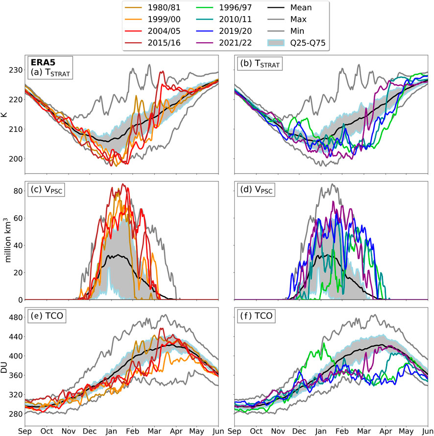
Figure 1. Evolution of the Northern polar cap (60$°$–90$°$N) zonal mean (a,b) stratospheric temperature (T_STRAT, calculated following Equation 1), (c,d) volume of polar stratospheric clouds (V_PSC, calculated following Equation 2) and (e,f) total column ozone (TCO). All data from ERA5 spanning September 1980 to June 2024. Colored lines mark selected years with particularly cold stratospheric temperatures early (1980/81 (gold), 1999/00 (orange), 2004/05 (red), 2015/16 (brown)) or late (1996/97 (light green), 2010/11 (dark green), 2019/20 (blue), 2021/22 (purple)) in the season. Additional solid lines illustrate the long-term mean (black) and the envelope of daily minima and maxima (grey). The interquartile range (Q25-Q75) is given in grey shading with blue envelope.

This disconnection between early and late winter conditions is exemplified e.g., by the widely studied winter seasons 2010/11 and 2019/20 that showed record low ozone in Arctic spring compared to the winters 2015/16 and 2004/2005 which started out anomalously cold, but due to stratospheric sudden warmings substantial ozone loss was undercut mid-season. Following the large ozone losses occurring in 2010/11, the cold early wintertime stratospheric temperatures in the 2015/16 season received close attention by the scientific community (e.g., Khosrawi et al., 2017; Manney and Lawrence, 2016). Large fractions of the northern polar cap were particularly cold, and early January was the coldest in the observational record. Despite these cold conditions early in the season, springtime ozone columns were far above average, as a consequence of a major SSW that caused temperatures in the LS and MS to rise about 12 K within a few days (see Supplementary Figures S2a,c, S3 a,c) and the area with T $<$ T_NAT almost halved (see Figure 1c; Supplementary Figure S1c). After a short interruption, the warming event continued. By mid February, the V_PSC proxy had collapsed to less than 20 million km³ and polar cap average air temperature in the LS was much warmer, about 214 K. Despite a short cooling period thereafter, this warming was strong enough to destabilize the vortex, and by March stratospheric temperatures were well above (and V_PSC well below) the long-term average.

In contrast temperatures in 2010/11 were only slightly below average in early winter (see Figure 1B; Supplementary Figure S1b), but cooled strongly thereafter, and cold conditions persisted till April causing widespread ozone loss (e.g., Manney et al., 2011; Hand, 2016). A similar evolution of very cold polar stratospheric springtime conditions, with even larger PSC abundances (absolute highest V_PSC values from beginning to mid-March 2020) and exceptional low springtime TCO (see Figures 1B,D,F; Supplementary Figures S1b,d,f) was observed in the season of 2019/20 (e.g., Kuttippurath et al., 2021; Ardra et al., 2022).

These years stand as examples for the wide variability of Arctic polar stratospheric conditions and motivate the main question of our study: can springtime ozone columns be predicted from conditions early in the winter, and if so through which covariate(s) and with which lead times?

3.2 Correlation analysis

To answer this question we focus on the extended winter season, which we define as December 1st to March 31st. Over this period we consider pairwise correlations of T (or A_PSC) with O₃ in the LS and MS (defined as 50 hPa and 30 hPa level, respectively) as well as the T_STRAT and PSC proxies with TCO. The period of interest for O₃ and TCO is the March mean (hereinafter indicated in figures with subscript M) and using T, A_PSC, V_PSC, and T_STRAT as predictors, we consider temporal averages over 31–121 days starting from December 1st (spanning the months of December, January, February, and March). For all other start dates the predictor window widths range from 31 days up to the number of days left until March 31st.

Figures 2a,c,e show correlograms for the temperature and ozone metrics. We start with one of our key findings: correlation coefficients between T and O₃ in the LS are insignificant (and small, i.e., $R<0.3$) for predictors spanning only early winter (December and January). This period holds no predictive power for springtime ozone. In the MS insignificant correlations persist even longer (till mid-February). For both the LS and MS significant correlations exceeding 0.6 emerge only if March conditions are considered, but this indicates no predictive power, only that March temperatures are correlated with March ozone. In summary, these results suggest that T is not a particularly good predictor for ozone in the LS and MS, and especially not early winter T. The same result applies for T_STRAT (which is dominated by T at 50 hPa) and its correlation with March TCO (panel e). We note in passing that similar results are found for ERA5 equivalent latitude calculations (Supplementary Figure S4) and with MERRA2 (Supplementary Figure S5).

Figure 2

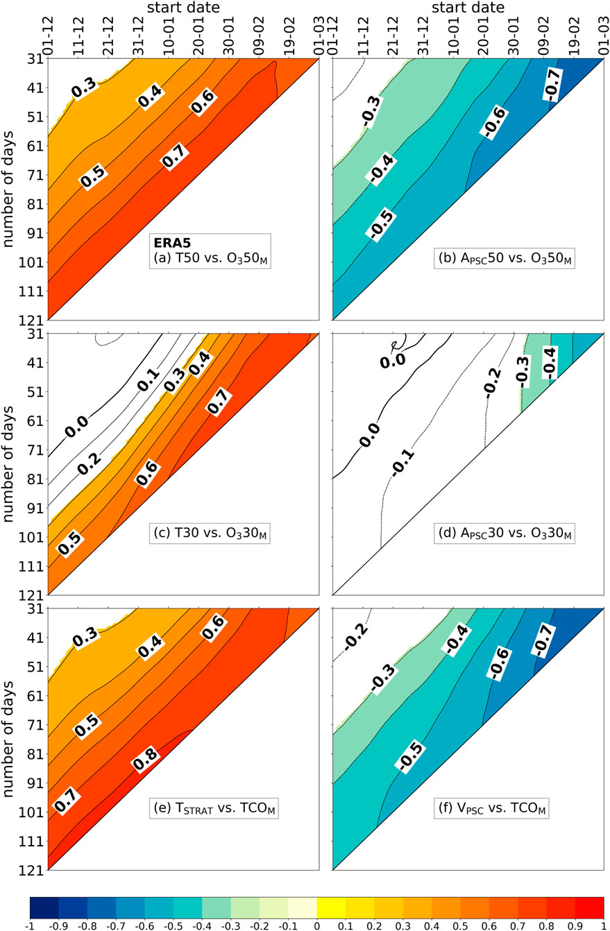
Figure 2. Correlograms between Northern polar cap (a) temperature and March mean ozone mixing ratio at 50 hPa, (b) A_PSC and March mean ozone mixing ratio at 50 hPa, (c,d) as (a,b) but for 30 hPa, (e) T_STRAT and March mean column ozone content, (f) V_PSC and March mean column ozone content. Temperature and PSC metrics are calculated in all panels as temporal averages spanning 31–121 days starting from December 1st. Ozone metrics are calculated as March arithmetic means (indicated with subscript M). Color-coding indicates a statistically significant correlation at the 95% confidence level. All data are from ERA5 spanning winter-spring seasons from December 1980 to March 2024.

It is possible, however, that stronger correlations might emerge between O₃ (TCO) and temperature extremes, as captured by the A_PSC (or V_PSC) proxies which are frequently considered in seasonal ozone prediction studies (e.g., Rex et al., 2006). Figures 2b,d,f, show that this is not the case. Overall, correlations are even weaker for PSC proxies and March ozone. Here too, as shown above for temperature, PSC proxies hold no predictive power for March ozone if only early winter conditions (December and/or January) are considered. Our analysis, therefore, supports the view that polar cap T, while severely limited in predictive power, is a better indicator of Arctic stratospheric conditions relevant for ozone changes than A_PSC or V_PSC, confirming the findings of Rieder et al. (2014).

Motivated by these findings, one might wonder if another covariate might be a better predictor for springtime O₃ content than T or PSC proxies. A natural candidate might be ozone concentrations earlier in the season, as these integrate both the chemical and dynamical conditions over the Arctic polar cap. We evaluate this hypothesis in Figures 3a–c, where we show correlograms for O₃ (and TCO) in March and preceding predictor windows for ERA5 (results in equivalent latitudes and for MERRA2 are comparable, and given in Supplementary Figures S6a–c; Supplementary Figures S7a–c). While qualitatively the results are similar as for T as predictor (compare Figure 2), these correlations are substantially higher. This is particularly true for predictor windows starting in early February and beyond. The highest correlations are, however, still found for predictors including March observations, indicating limitations in long-term predictive power.

Figure 3

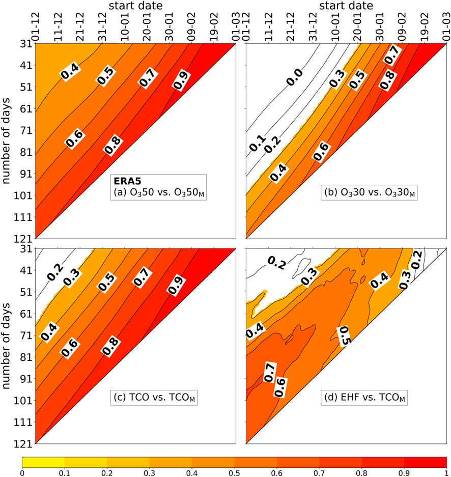
Figure 3. Correlograms between Northern polar cap (a) ozone mixing ratio and March mean ozone mixing ratio at 50 hPa, (b) as (a) but for 30 hPa, (c) for column ozone content and March mean column ozone content, (d) eddy heat flux and March mean column ozone content. Predictor metrics are calculated in all panels as temporal averages spanning 31–121 days starting from December 1st. Target ozone metrics are calculated as March arithmetic means (indicated with subscript M). Color-coding indicates a statistically significant correlation at the 95% confidence level. All data are from ERA5 spanning December 1980 to March 2024.

Another potential predictor for Arctic ozone abundances is eddy heat flux (EHF) at 100 hPa, which has been widely utilized to characterize wave influence on the vortex state and the Brewer-Dobson Circulation and thus ozone transport (e.g., Weber et al., 2011; Friedel et al., 2023). A correlogram between EHF and TCO is given in Figure 3d (and for MERRA2 in Supplementary Figure S6d). In contrast to the other predictors, which show their highest correlations with March ozone in late winter/early spring (mid-February to March), EHF displays no significant values in that particular time frame. The highest correlations with EHF occur when a long integration period (at least December to mid February) is considered and the starting day of the input data is not after 1st of January. Our results indicate that on shorter lead times EHF does not emerge as powerful predictor.

3.3 Predictive skill of ozone covariates

To further illustrate the predictive skill of the individual covariates discussed above, we show linear regression model predictions for stratospheric March polar cap mean total column ozone (TCO_M) based on T_STRAT, V_PSC, EHF, or TCO for ERA5 in Figure 4 (for MERRA2 in Supplementary Figure S8). We do so for four selected predictor windows, each spanning 31 days: one each in early (December 15th–January 14th), mid (January 15th - February 14th), and late winter (January 28th–February 27th) and the winter spring transition (February 14th - March 16th). Note that these 31 days intervals are chosen as examples, and that neighboring predictors yield similar results (see Figure 2 and Supplementary Figure S5).

Figure 4

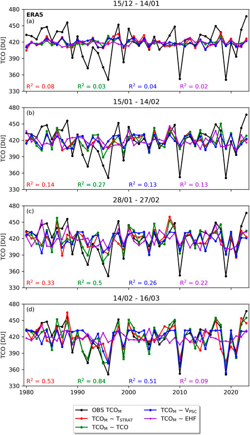
Figure 4. Comparison of observed (black) and predicted (color coded) March Northern polar cap total column ozone (TCO_M) based on 31 days averages of T_STRAT (red), TCO (green), V_PSC (blue) or EHF (purple). All predictors are calculated over 31 days time windows: (a) December 15 - January 14, (b) January 15 - February 14, (c) January 28 - February 27, (d) February 14 - March 16. Explained variance $({\mathrm{R}}^{\mathrm{2}})$ of TCO_M for individual predictors is provided color coded at the bottom of the panels. All data are from ERA5 spanning December 1980 to March 2024.

Generally for all predictors, except EHF (which holds the least predictive power), we find that the further the predictor window is away from March the lower the explained TCO_M variance becomes. Using V_PSC as a predictor, the explained variance for the first three predictor windows is at/below 30% (see Figures 4a–c). Only the last window, which includes more than half of the days for March, shows improved explained variance but still just above 50% (Figure 4d). T_STRAT as a predictor yields a slightly higher explained variance then V_PSC for all predictor windows. EHF as a predictor is always below 25% explanatory power in the TCO_M variance (Figures 4a–c). In contrast, TCO yields substantially higher explained variance scores throughout all four predictor windows: up to twice as large as T_STRAT or V_PSC. Using TCO itself as a predictor during the winter-spring transition yields an explained variance of more than 80% (Figure 4d), mid-winter TCO still an explained variance of 50%. Thus, although pronounced residuals between predictions and observations remain in individual years, TCO emerges as most promising predictor variable for Arctic springtime ozone columns in the set analyzed here.

4 Discussion and conclusion

In this paper, we have asked the question whether springtime Arctic ozone columns are predictable from wintertime conditions. To this end we have examined two reanalyses (ERA5, MERRA2) for the period 1980–2024 to determine if the mean polar cap stratospheric temperature (T_STRAT,T₅₀, T₃₀), PSC proxies (A_PSC and V_PSC), and eddy heat flux (EHF) are skillfull predictors for ozone in Arctic spring.

Our results show that Arctic springtime ozone can only be predicted with short lead-time, and even then with limited accuracy. Furthermore, temperature proxies which have been repeatedly employed in the literature emerge as rather inadequate predictors for springtime ozone. Similarly wintertime EHF does not emerge as a skillful predictor. In contrast, ozone itself shows the highest predictive skill, particularly around the winter-spring transition but also already earlier in the season. That said, while ozone performs best across the analyzed predictors, here too strong limitations to predictive skill apply. Our results indicate that observations during the winter season have limited value as predictors for the state of the Arctic ozone layer in spring. As we have shown above, the predictive skill of statistical models (based on observations) is limited. Further research is needed in the field of chemistry-climate modelling to improve the accuracy of ensemble predictions based on the chemical and dynamical history of the ozone layer during winter and spring.

Data availability statement

All processed data files for this study are provided via Mendeley Data (Kuchar and Kult-Herdin, 2025), and all codes to reproduce the figures of this study are provided via Zenodo (Kuchar, 2025).

Author contributions

HR: Conceptualization, Formal Analysis, Investigation, Methodology, Project administration, Resources, Supervision, Writing – original draft, Writing – review and editing. JK-H: Data curation, Formal Analysis, Investigation, Methodology, Visualization, Writing – review and editing. LP: Conceptualization, Investigation, Methodology, Writing – review and editing. SS: Conceptualization, Investigation, Methodology, Writing – review and editing. AK: Data curation, Formal Analysis, Investigation, Methodology, Visualization, Writing – review and editing.

Funding

The author(s) declare that financial support was received for the research and/or publication of this article. HR and AK acknowledge support by BOKU University. LP is supported, in part, by a grant from the US National Science Foundation to Columbia University.

Acknowledgments

For ERA5 processing, resources have been used at the Deutsches Klimarechenzentrum (DKRZ) under project ID bd1022. We also acknowledge the MERRA2 reanalysis dataset provided by Martineau (2022) referred as the Reanalysis Intercomparison Dataset (RID). HR acknowledges fruitful discussions with J. Fritzer. The authors thank the referees for their comments.

Conflict of interest

The authors declare that the research was conducted in the absence of any commercial or financial relationships that could be construed as a potential conflict of interest.

Generative AI statement

The author(s) declare that no Generative AI was used in the creation of this manuscript.

Any alternative text (alt text) provided alongside figures in this article has been generated by Frontiers with the support of artificial intelligence and reasonable efforts have been made to ensure accuracy, including review by the authors wherever possible. If you identify any issues, please contact us.

Publisher’s note

All claims expressed in this article are solely those of the authors and do not necessarily represent those of their affiliated organizations, or those of the publisher, the editors and the reviewers. Any product that may be evaluated in this article, or claim that may be made by its manufacturer, is not guaranteed or endorsed by the publisher.

Supplementary material

The Supplementary Material for this article can be found online at: https://www.frontiersin.org/articles/10.3389/feart.2025.1610651/full#supplementary-material

References

Amos, M., Young, P. J., Hosking, J. S., Lamarque, J. F., Abraham, N. L., Akiyoshi, H., et al. (2020). Projecting ozone hole recovery using an ensemble of chemistry–climate models weighted by model performance and independence. Atmos. Chem. Phys. 20, 9961–9977. doi:10.5194/acp-20-9961-2020

CrossRef Full Text | Google Scholar

Ardra, A., Kuttippurath, J., Roy, R., Kumar, P., Raj, S., Müller, R., et al. (2022). The unprecedented ozone loss in the arctic winter and spring of 2010/2011 and 2019/2020. ACS Earth Space Chem. 6, 683–693. doi:10.1021/acsearthspacechem.1c00333

CrossRef Full Text | Google Scholar

Ayarzagüena, B., Langematz, U., Meul, S., Oberländer, S., Abalichin, J., and Kubin, A. (2013). The role of climate change and ozone recovery for the future timing of major stratospheric warmings. Geophys. Res. Lett. 40, 2460–2465. doi:10.1002/grl.50477

CrossRef Full Text | Google Scholar

Ayarzagüena, B., Polvani, L. M., Langematz, U., Akiyoshi, H., Bekki, S., Butchart, N., et al. (2018). No robust evidence of future changes in major stratospheric sudden warmings: a multi-model assessment from CCMI. Atmos. Chem. Phys. Discuss., 1–17. doi:10.5194/acp-2018-296

CrossRef Full Text | Google Scholar

Baldwin, M. P., Ayarzagüena, B., Birner, T., Butchart, N., Butler, A. H., Charlton-Perez, A. J., et al. (2021). Sudden stratospheric warmings. Rev. Geophys. 59, e2020RG000708. doi:10.1029/2020RG000708

CrossRef Full Text | Google Scholar

Butler, A. H., Sjoberg, J. P., Seidel, D. J., and Rosenlof, K. H. (2017). A sudden stratospheric warming compendium. Earth Syst. Sci. Data 9, 63–76. doi:10.5194/essd-9-63-2017

CrossRef Full Text | Google Scholar

Dhomse, S., Kinnison, D., Chipperfield, M. P., Cionni, I., Hegglin, M., Abraham, N. L., et al. (2018). Estimates of ozone return dates from chemistry-climate model initiative simulations. Atmos. Chem. Phys. Discuss. 18, 8409–8438. doi:10.5194/acp-2018-87

CrossRef Full Text | Google Scholar

Eyring, V., Cionni, I., Bodeker, G. E., Charlton-Perez, A. J., Kinnison, D. E., Scinocca, J. F., et al. (2010). Multi-model assessment of stratospheric ozone return dates and ozone recovery in CCMVal-2 models. Atmos. Chem. Phys. 10, 9451–9472. doi:10.5194/acp-10-9451-2010

CrossRef Full Text | Google Scholar

Farman, J. C., Gardiner, B. G., and Shanklin, J. D. (1985). Large losses of total ozone in Antarctica reveal seasonal CLOX/NOX interaction. Nature 315, 207–210. doi:10.1038/315207a0

CrossRef Full Text | Google Scholar

Friedel, M., Chiodo, G., Stenke, A., Domeisen, D. I. V., and Peter, T. (2022). Effects of Arctic ozone on the stratospheric spring onset and its surface impact. Atmos. Chem. Phys. 22, 13997–14017. doi:10.5194/acp-22-13997-2022

CrossRef Full Text | Google Scholar

Friedel, M., Chiodo, G., Sukhodolov, T., Keeble, J., Peter, T., Seeber, S., et al. (2023). Weakening of springtime Arctic ozone depletion with climate change. Atmos. Chem. Phys. 23, 10235–10254. doi:10.5194/acp-23-10235-2023

CrossRef Full Text | Google Scholar

Gelaro, R., McCarty, W., Suárez, M. J., Todling, R., Molod, A., Takacs, L., et al. (2017). The modern-Era Retrospective analysis for research and Applications, version 2 (MERRA-2). J. Clim. 30, 5419–5454. doi:10.1175/jcli-d-16-0758.1

PubMed Abstract | CrossRef Full Text | Google Scholar

Hand, E. (2016). Record ozone hole may open over Arctic in the spring. Science 351, 650. doi:10.1126/science.351.6274.650

PubMed Abstract | CrossRef Full Text | Google Scholar

Hanson, D., and Mauersberger, K. (1988). Laboratory studies of the nitric acid trihydrate: implications for the south polar stratosphere. Geophys. Res. Lett. 15, 855–858. doi:10.1029/GL015i008p00855

CrossRef Full Text | Google Scholar

Hersbach, H., Bell, B., Berrisford, P., Hirahara, S., Horányi, A., Muñoz-Sabater, J., et al. (2020). The ERA5 global reanalysis. Q. J. Roy. Meteor Soc. 146, 1999–2049. doi:10.1002/qj.3803

CrossRef Full Text | Google Scholar

Khosrawi, F., Kirner, O., Sinnhuber, B. M., Johansson, S., Höpfner, M., Santee, M. L., et al. (2017). Denitrification, dehydration and ozone loss during the 2015/2016 Arctic winter. Atmos. Chem. Phys. 17, 12893–12910. doi:10.5194/acp-17-12893-2017

CrossRef Full Text | Google Scholar

Kuchar, A., and Kult-Herdin, J. (2025). Accompanying data to “Are springtime Arctic ozone concentrations predictable from wintertime conditions?”. Mendeley Data. doi:10.17632/ts4brdbx2h.1

CrossRef Full Text | Google Scholar

Kuchar, A. (2025). BOKU-Meteo/springtime-arctic-ozone: first release of our code repository related to springtime arctic ozone. Zenodo. doi:10.5281/zenodo.14882480

CrossRef Full Text | Google Scholar

Kuttippurath, J., Godin-Beekmann, S., Lefèvre, F., Nikulin, G., Santee, M. L., and Froidevaux, L. (2012). Record-breaking ozone loss in the Arctic winter 2010/2011: comparison with 1996/1997. Atmos. Chem. Phys. 12, 7073–7085. doi:10.5194/acp-12-7073-2012

CrossRef Full Text | Google Scholar

Kuttippurath, J., Feng, W., Müller, R., Kumar, P., Raj, S., Gopikrishnan, G. P., et al. (2021). Exceptional loss in ozone in the Arctic winter/spring of 2019/2020. Atmos. Chem. Phys. 21, 14019–14037. doi:10.5194/acp-21-14019-2021

CrossRef Full Text | Google Scholar

Langematz, U., Meul, S., Grunow, K., Romanowsky, E., Oberländer, S., Abalichin, J., et al. (2014). Future Arctic temperature and ozone: the role of stratospheric composition changes. J. Geophys. Res. Atmos. 119, 2092–2112. doi:10.1002/2013JD021100

CrossRef Full Text | Google Scholar

Manney, G. L., and Lawrence, Z. D. (2016). The major stratospheric final warming in 2016: dispersal of vortex air and termination of Arctic chemical ozone loss. Atmos. Chem. Phys. 16, 15371–15396. doi:10.5194/acp-16-15371-2016

CrossRef Full Text | Google Scholar

Manney, G. L., Santee, M. L., Rex, M., Livesey, N. J., Pitts, M. C., Veefkind, P., et al. (2011). Unprecedented Arctic ozone loss in 2011. Nature 478, 469–475. doi:10.1038/nature10556

PubMed Abstract | CrossRef Full Text | Google Scholar

Martineau, P. (2022). Reanalysis Intercomparison dataset (RID), Japan agency for marine-earth science and technology. Available online at: https://www.jamstec.go.jp/RID/thredds/catalog/catalog.html.

Google Scholar

Matthias, V., Dörnbrack, A., and Stober, G. (2016). The extraordinarily strong and cold polar vortex in the early northern winter 2015/2016. Geophys. Res. Lett. 43, 121287–212294. doi:10.1002/2016GL071676

CrossRef Full Text | Google Scholar

Mitchell, D. M., Osprey, S. M., Gray, L. J., Butchart, N., Hardiman, S. C., Charlton-Perez, A. J., et al. (2012). The effect of climate change on the variability of the northern hemisphere stratospheric polar vortex. J. Atmos. Sci. 69, 2608–2618. doi:10.1175/jas-d-12-021.1

CrossRef Full Text | Google Scholar

Montzka, S. A., Butler, J. H., Myers, R. C., Thompson, T. M., Swanson, T. H., Clarke, A. D., et al. (1996). Decline in the tropospheric abundance of halogen from halocarbons: implications for stratospheric ozone depletion. Science 272, 1318–1322. doi:10.1126/science.272.5266.1318

PubMed Abstract | CrossRef Full Text | Google Scholar

Montzka, S. A., Butler, J. H., Elkins, J., Thompson, T. M., Clarke, A. D., and Lock, L. T. (1999). Present and future trends in the atmospheric burden of ozone-depleting halogens. Nature 398, 690–694. doi:10.1038/19499

CrossRef Full Text | Google Scholar

Morgenstern, O., Hegglin, M. I., Rozanov, E., O'Connor, F. M., Abraham, N. L., Akiyoshi, H., et al. (2017). Review of the global models used within phase 1 of the Chemistry-Climate Model Initiative (CCMI). Geosci. Model Dev. 10, 639–671. doi:10.5194/gmd-10-639-2017

CrossRef Full Text | Google Scholar

Müller, R., Grooß, J.-U., Lemmen, C., Heinze, D., Dameris, M., and Bodeker, G. (2008). Simple measures of ozone depletion in the polar stratosphere. Atmos. Chem. Phys. 8, 251–264. doi:10.5194/acp-8-251-2008

CrossRef Full Text | Google Scholar

Nash, E. R., Newman, P. A., Rosenfield, J. E., and Schoeberl, M. R. (1996). An objective determination of the polar vortex using Ertel’s potential vorticity. J. Geophys. Res. Atmos. 101, 9471–9478. doi:10.1029/96JD00066

CrossRef Full Text | Google Scholar

Newman, P. A., Nash, E. R., and Rosenfield, J. E. (2001). What controls the temperature of the Arctic stratosphere during the spring? J. Geophys. Res. Atmos. 106, 19999–20010. doi:10.1029/2000JD000061

CrossRef Full Text | Google Scholar

Peter, T. (1997). Microphysics and heterogeneous chemistry of polar stratospheric clouds. Annu. Rev. Phys. Chem. 48, 785–822. doi:10.1146/annurev.physchem.48.1.785

PubMed Abstract | CrossRef Full Text | Google Scholar

Polvani, L. M., Keeble, J., Banerjee, A., Checa-Garcia, R., Chiodo, G., Rieder, H., et al. (2023). No evidence of worsening Arctic springtime ozone losses over the 21st century. Nat. Commun. 14, 1608. doi:10.1038/s41467-023-37134-3

PubMed Abstract | CrossRef Full Text | Google Scholar

Pommerau, J. P., Goutail, F., Lefèvre, F., Pazmino, A., Adams, C., Dorokhov, V., et al. (2013). Why unprecedented ozone loss in the Arctic in 2011? Is it related to climatic change? Atmos. Chem. Phys. 13, 5299–5308. doi:10.5194/acp-13-5299-2013

CrossRef Full Text | Google Scholar

Rex, M., Salawitch, R. J., von der Gathen, P., Harris, N. R. P., Chipperfield, M. P., and Naujokat, B. (2004). Arctic ozone loss and climate change. Geophys. Res. Lett. 31. doi:10.1029/2003GL018844

CrossRef Full Text | Google Scholar

Rex, M., Salawitch, R. J., Deckelmann, H., von der Gathen, P., Harris, N. R. P., Chipperfield, M. P., et al. (2006). Arctic winter 2005: implications for stratospheric ozone loss and climate change. Geophys. Res. Lett. 33. doi:10.1029/2006GL026731

CrossRef Full Text | Google Scholar

Rieder, H. E., and Polvani, L. M. (2013). Are recent Arctic ozone losses caused by increasing greenhouse gases? Geophys. Res. Lett. 40, 4437–4441. doi:10.1002/Grl.50835

CrossRef Full Text | Google Scholar

Rieder, H. E., Polvani, L. M., and Solomon, S. (2014). Distinguishing the impacts of ozone-depleting substances and well-mixed greenhouse gases on Arctic stratospheric ozone and temperature trends. Geophys. Res. Lett. 41, 2652–2660. doi:10.1002/2014gl059367

CrossRef Full Text | Google Scholar

Solomon, S. (1999). Stratospheric ozone depletion: a review of concepts and history. Rev. Geophys. 37, 275–316. doi:10.1029/1999rg900008

CrossRef Full Text | Google Scholar

Solomon, S., Garcia, R. R., Rowland, F. S., and Wuebbles, D. J. (1986). On the depletion of Antarctic ozone. Nature 321, 755–758. doi:10.1038/321755a0

CrossRef Full Text | Google Scholar

Solomon, S., Haskins, J., Ivy, D. J., and Min, F. (2014). Fundamental differences between Arctic and Antarctic ozone depletion. Proc. Natl. Acad. Sci. 111, 6220–6225. doi:10.1073/pnas.1319307111

PubMed Abstract | CrossRef Full Text | Google Scholar

SPARC-CCMVal (2010). SPARC report on the evaluation of chemistry-climate models. Technical Report.

Google Scholar

Voigt, C., Dörnbrack, A., Wirth, M., Groß, S. M., Baumann, R., Ehard, B., et al. (2016). Widespread persistent polar stratospheric ice clouds in the Arctic. Atmos. Chem. Phys. Discuss., 1–27. doi:10.5194/acp-2016-1082

CrossRef Full Text | Google Scholar

von der Gathen, P., Kivi, R., Wohltmann, I., Salawitch, R. J., and Rex, M. (2021). Climate change favours large seasonal loss of Arctic ozone. Nat. Commun. 12, 3886. doi:10.1038/s41467-021-24089-6

PubMed Abstract | CrossRef Full Text | Google Scholar

Weber, M., Dikty, S., Burrows, J. P., Garny, H., Dameris, M., Kubin, A., et al. (2011). The Brewer-Dobson circulation and total ozone from seasonal to decadal time scales. Atmos. Chem. Phys. 11, 11221–11235. doi:10.5194/acp-11-11221-2011

CrossRef Full Text | Google Scholar

WMO (2022). Scientific assessment of ozone depletion: 2022. Technical Report.

Google Scholar