Assessment of slope stability based on the improved entropy weight-gray target theory

Landslides are a serious natural hazard globally. While the traditional grey target model has long served as an effective tool for slope stability assessment, its predictive accuracy remains questionable due to the inherent correlations among evaluation indicators. To mitigate this limitation, this study introduces an enhanced entropy weight-grey target theory for slope stability evaluation. The proposed model innovates in two key aspects: first, it substitutes the covariance matrix in the Mahalanobis distance calculation with a correlation coefficient matrix, thereby addressing indicator interdependencies; second, it adapts the positive and negative ideal solutions from the TOPSIS model to define the corresponding target centers in the grey target framework. The improved model’s efficacy is validated through an engineering case study. The findings confirm that the proposed method not only offers a feasible approach for slope stability assessment but also demonstrates superior predictive accuracy to the traditional grey target model. This research contributes a novel methodology and conceptual framework for future slope stability evaluations.

1 Introduction

Landslides are one of the most frequent accidents in opencast mines. They pose a direct threat to people’s lives and property safety (Gu et al., 2021a; Zhao et al., 2021; Zhao et al., 2023; Zhao et al., 2022a). Developing an accurate and applicable slope stability evaluation model holds great theoretical significance and practical utility for mitigating landslide risks. Due to the randomness, fuzziness, and variability of the factors influencing slope stability, considerable uncertainty in slope stability evaluation exist, and this uncertainty poses difficulties for the assessment and prediction of slope stability (Gu and Wu, 2019; Zhao et al., 2019a; Zhao et al., 2019b; Zhao and Liu, 2012; Zhao et al., 2022b).

Currently, numerous scholars extensively employ methods such as the material point method (WANG et al., 2017), set pair analysis (LIU, 2014), particle swarm optimization (DONG, 2016), and artificial neural networks (Yuansong et al., 2013) to evaluate slope stability. Yongqiang et al. (2007) also applied the Projection Pursuit Algorithm to assess slope stability and proposed the Projection Pursuit Classification (PPC) evaluation method. Wang et al. (2019) proposed an evaluation method based on genetic algorithm and projection pursuit and conducted an empirical study on the slope stability of an opencast mine in the Tangshan area. Yang et al. (2018) introduced the cloud model theory into the slope stability evaluation based on the traditional fuzzy comprehensive evaluation method and achieved better assessment results. Jianye et al. (2019) introduced the concept of cloud into slope stability evaluation and established a set pair cloud model to evaluate slope stability. Fang and Shang (2019) established an evaluation model for slope stability of open-pit mines based on game theory and the cloud model. Jun et al. (2016) constructed a model for evaluating slope stability by utilizing the harmonious particle swarm optimization algorithm in conjunction with the feedforward neural network model. Botao et al. (2016) proposed a material point strength reduction method for slope stability evaluation from the perspective of stress and strain within the slope. However, the influence factors of slope stability are complex and highly uncertain, all of which can affect the accuracy of an evaluation. The risk assessment of slope is essentially a multi-indicator problem with uncertainties, so the grey target model can be considered to evaluate the risk level of slope (Gu et al., 2021b; Gu et al., 2021c). However, the suggested model must still be improved. In the traditional grey target model, the target distance is calculated using Euclidean distance, without considering the correlation between evaluation indicators, which may also affect the accuracy of the evaluation results (Gu et al., 2022).

To overcome the above shortcomings, the improved entropy weight-grey target theory is introduced to assess the slope stability. It is a combination of the entropy weight method and grey target theory. It can effectively handle complex, numerous, and highly correlated research objects. To effectively combine the entropy method with the grey target model (Gu and Wu, 2016), this article improves the traditional grey target evaluation model from two aspects: ① the correlation coefficient matrix is adopted to replace the covariance matrix in the Mahalanobis distance; ② the positive and negative ideal solutions in the TOPSIS model are introduced to define the positive and negative target centers.

The article is organized as follows: in Section 2, theory and methodology based on the entropy weight-grey target theory are presented; in Section 3, the engineering background is introduced; in Section 4, the assessment model is constructed, and the assessment results are analyzed; in Section 5, conclusions are drawn.

2 Methodology

2.1 The improved entropy weight-grey target model

Compared to the traditional model, the improved model can enhance the predictive accuracy of slope risk level. The assessment flowchart is plotted in Figure 1.

Figure 1

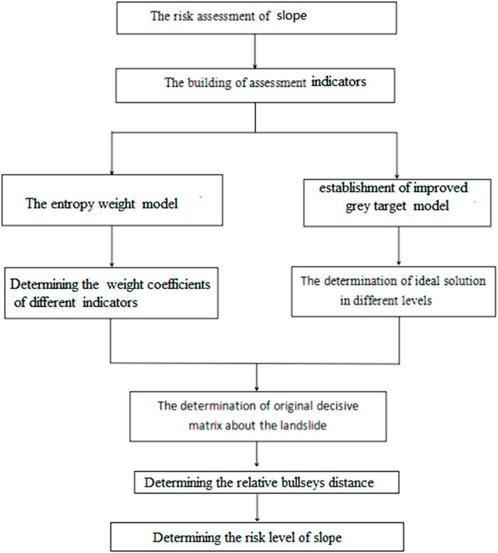
Figure 1. Evaluation flowchart of the improved grey target model.

2.2 The entropy weight method

The basic principle of the entropy weight method (EW) (Zhang and Yang, 2018) is to measure the randomness degree of a system using entropy values. The more information the elements a system contains, the less uncertainty there is. Namely, for each evaluation indicator, the greater the data variability it contains, the more information it encompasses, and the greater its impact on the evaluation results will be; consequently, a relatively higher weight is assigned to it. Its calculative procedure is listed as follows:

① constructing the original matrix of samples $X=\left(x_{ij}\right)\left(i=1,2,3,...,m;j=1,2,3,...,n\right)$

② standardizing the original matrix

The standardization is shown as follows:

$B_{nm}=\left(b_{ij}\right)(1)$

For the benefit-type indicators (Jun et al., 2016):

$b_{ij}=\frac{a_{ij}-\mathit{min}\left(a_{ij}\right)}{\underset{j}{\mathit{max}}\left(a_{ij}\right)-\underset{j}{\mathit{min}}\left(a_{ij}\right)}(2)$

For the cost-type indicators:

$b_{ij}=\frac{\max \left(a_{\text{ij}}\right)-a_{ij}}{\underset{j}{\mathit{max}}\left(a_{ij}\right)-\underset{j}{\mathit{min}}\left(a_{ij}\right)}(3)$

③ the calculation of information entropy

$E_j=-\raisebox{1ex}{${\displaystyle {\sum }_{i=1}^n}{g}_{ij}\mathit{ln}{g}_{ij}$}\!\left/ \!\raisebox{-1ex}{$\mathit{ln}n$}\right.\left(j=1,2,...,m\right)(4)$

$g_{ij}=\frac{1+b_{ij}}{{\displaystyle {\sum }_{i=1}^n}\left(1+b_{ij}\right)}(5)$

Where $E_j$-information entropy

$g_{ij}$-proportion of characteristic value

④ The calculation of weight coefficients

${\omega }_j=\frac{1-E_j}{m-{\displaystyle {\sum }_{j=1}^m}{E}_j}(6)$

2.3 The Mahalanobis distance calculation method based on the correlation coefficient matrix

To accurately characterize the correlation between evaluation indicators, the correlation coefficient matrix replaces the covariance matrix in the Mahalanobis distance and is introduced into the traditional grey target model. Simultaneously, during the calculation process of the target center in the traditional grey target model, a grey target is defined under the condition of no standard mode. The ideal optimal value serves the target center (Xue-bin and Chang-liang, 2007; Gu et al., 2025). The distances from each sample to the target center are then calculated, and the sample ranking and ordering are determined by comparing the sizes of these distances. However, only a single ideal optimal value is the target center. In that case, explaining the ranking and ordering of samples becomes difficult when multiple samples have the same or similar distances to the target center. Therefore, the positive and negative ideal solutions are introduced from the TOPSIS model to define positive and negative target centers. When multiple samples have the same or similar distances to the target center, the ranking and ordering of samples can be determined by further evaluating their distances to the worst target center. Simultaneously, the Mahalanobis distance based on the correlation coefficient is used to calculate the positive and negative target center distances. The relative target center distance is then defined to determine the risk level and ranking. The calculation steps are as follows:

1. The construction of the sample matrix

It is assumed that there are $m$ samples in the sample set $X=\left(\begin{array}{ccccc}{x}_1& x_2& x_3& ...& x_m\end{array}\right)$. $n$ evaluation indicators construct the assessment indicator set $V=\left(\begin{array}{ccccc}{v}_1& v_2& v_3& ...& v_n\end{array}\right)$. The magnitude of sample $x_k$ for evaluation indicator $v_l$ is $a_{kl}\left(k=1,2,3,...,m\right),\left(l=1,2,3,...,n\right)$, assuming that the sample indicator matrix of $X$ to $V$ is

$A=\left[\begin{array}{cccc}{a}_{11}& a_{12}& ...& a_{1n}\\ a_{21}& a_{22}& ...& a_{2n}\\ ...& ...& ...& ...\\ a_{m1}& a_{m2}& ...& a_{mn}\end{array}\right](7)$

2. The normalization of the sample indicator matrix

A linear transformation is applied to the sample indicator matrix A to perform standardization processing, unifying the dimensions of evaluation indicators.

Let the mean of the evaluation indicator be

$C_i=\frac{1}{m}{\displaystyle \sum _{k=1}^m}{a}_{kl}(8)$

For the cost-type indicator (Zhou et al., 2021):

$r_{kl}=\frac{c_l-a_{kl}}{\mathit{max}\left(\underset{1\le k\le m}{\mathit{max}}\left(a_{kl}\right)-c_l,c_l-\underset{1\le k\le m}{\mathit{min}}\left(a_{kl}\right)\right)}(9)$

For the benefit-type indicator:

$r_{kl}=\frac{a_{kl}-c_l}{\mathit{max}\left(\underset{1\le k\le m}{\mathit{max}}\left(a_{kl}\right)-c_l,c_l-\underset{1\le k\le m}{\mathit{min}}\left(a_{kl}\right)\right)}(10)$

According to the characteristics of the evaluation indicators, the sample indicator matrix $A$ can be transformed into a standardized sample indicator matrix $R$ using Equations 8–10:

$R=\left[\begin{array}{cccc}{r}_{11}& r_{12}& ...& r_{1n}\\ r_{21}& r_{22}& ...& r_{2n}\\ ...& ...& ...& ...\\ r_{n1}& r_{n2}& ...& r_{nn}\end{array}\right](11)$

3. The determination of the negative and positive target centers

Let $r_l^{+}=\mathit{max}\left\{\left.r_{kl}\right|1\le k\le n\right\}\left(l=1,2,...,n\right)$, then

$r^{+}=\left(\begin{array}{cccc}{r}_1^{+},& r_2^{+}& ...,& r_n^{+}\end{array}\right)(12)$

Where $r^{+}$ is the positive ideal solution; namely, it is the positive target center distance.

Let $r_l^{+}=\mathit{min}\left\{\left.r_{kl}\right|1\le k\le n\right\}\left(l=1,2,...,n\right)$, then:

$r^{-}=\left(\begin{array}{cccc}{r}_1^{-},& r_2^{-}& ...,& r_n^{-}\end{array}\right)$

Where $r^{-}$ is the positive ideal solution; namely, it is the negative target center distance;

4. The determination of positive and negative target center distance

Let:

$i_l={\omega }_i\left(r_{kl}-r_i^{+}\right),I={\left(\begin{array}{cccc}{i}_1& i_2& ...& i_n\end{array}\right)}^T(13)$

$j_l={\omega }_i\left(r_{kl}-r_i^{-}\right),J={\left(\begin{array}{cccc}{j}_1& j_2& ...& j_n\end{array}\right)}^T(14)$

Where $I$ and $J$ represent the weighted differences between sample $x_k$ and the positive and negative target centers, respectively.

The distance from sample $x_k$ to the positive target center, that is, the positive target center distance, is calculated based on the correlation coefficient matrix as follows:

${\epsilon }_k^{+}={\left(I^T{\prod }^{-1}I\right)}^{1/2}(15)$

Likely, the negative target center distance is

${\epsilon }_k^{-}={\left(J^T{\prod }^{-1}J\right)}^{1/2}(16)$

Where $II$ denotes the correlation coefficient matrix of the standardized sample indicator matrix $R$.

5. Determination of the relative target center distance

The bigger the relative target distance ${\xi }_k$, the higher the risk level. The relative target center distance of the $kth$ indicator is

${\epsilon }_k^{*}=\frac{{\epsilon }_k^{-}}{{\epsilon }_k^{+}+{\epsilon }_k^{-}}(17)$

6. The classification of risk level

7. Let the set $\epsilon$ represent the collection of relative target distances for all evaluation samples, namely, $\epsilon =\left(\begin{array}{cccc}{\epsilon }_1*,& {\epsilon }_2*& ...& {\epsilon }_m*\end{array}\right)$. The set $D$ is defined as the ordered intervals obtained by partitioning set $\epsilon$ based on $t$ risk levels, namely, $D=\left(\begin{array}{cccc}{d}_1& d_2& ...& d_l\end{array}\right)$. Let $1\le \varphi <t$, and $\varphi$ is the positive integer. Then, the clinic value of $dth$ risk level ${\gamma }_{\varphi }=\mathit{max}\left\{d_{\varphi }\right\},{\eta }_{\varphi }=\mathit{min}\left\{d_{\varphi }\right\}$, and the level classification $Y$ of the improved grey target model is

$I_{\varphi }=\mu {\gamma }_{\varphi }+\left(1-\mu \right){\eta }_{\varphi +1},\mu \in \left(0,1\right)(18)$

$Y=\left\{\frac{d}{0\le d_1<z_1,f_1\le d_2<z_{2,}...,z_{i-1}\le d_t<+\infty }\right\}(19)$

3 Engineering background

The Shizibao landslide is located in Fengjie County, Chongqing Province (Figure 2). It is situated in Tiefo Village, Kangle Town, and is distributed along the slope on the right bank of the Meixi River, a first-tier tributary of the Yangtze River. The landslide is divided into three independent units (Landslide #I, Landslide #II, and Landslide #III) based on their genetic relationships and main sliding directions. The total volume of the landslide is 102.5 × 10⁴ m³; it is categorized as a large-scale shallow soil landslide.

Figure 2

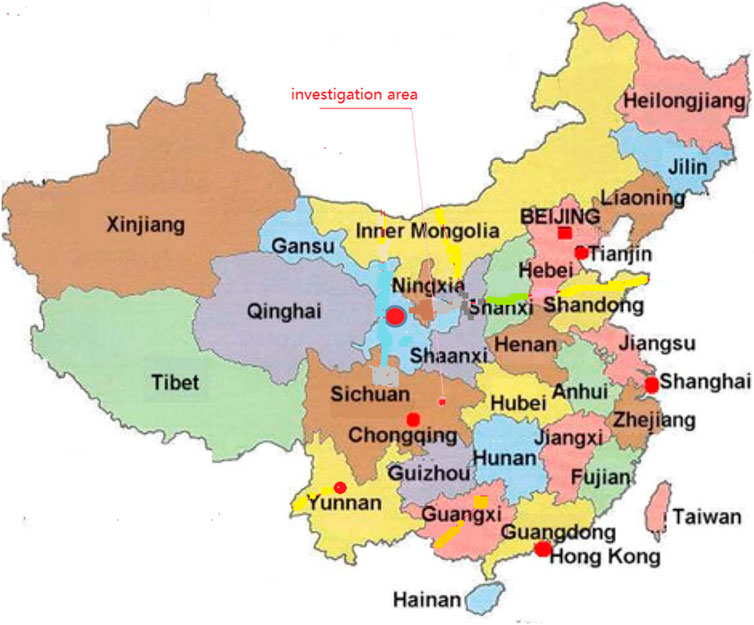
Figure 2. The location of the survey area.

The surveyed area belongs to the landform of low mountains and valleys formed by erosion. The overall terrain is higher in the southwest and lower in the northeast, with a wavy, undulating landscape. The highest point is located in the southwest, with an elevation of approximately 560 m. The lowest point is located in the Meixi River valley, with a water surface elevation of approximately 160 m and a relative height difference of 400 m. The rear part of the slope is a natural bedrock slope with a gradient of 35°–42°, while the front part of the slope is the bedrock bank slope of the Meixi River, with a gradient of 28°–46°. In some areas, gentle slopes with slope angles of 15°–22° are formed due to accumulations. Certain gullies in the exploration area are relatively developed, with narrow valley slopes and seasonal water flow within the gullies.

4 Establishing the assessment model

4.1 Constructing the indicator system

Numerous factors affect slope stability. Previous studies have primarily focused on balancing hazards and management, with an emphasis on the latter. However, preventing accidents is more about addressing the root causes of the problem. Indicators can be selected from three aspects of the inherent properties of slopes: rock mass structural planes, topography and landforms, and rock mechanical properties. Therefore, to establish an indicator system for slope stability, based on previous research findings (Zhou et al., 2008; Shou et al., 2024), six indicators that have a significant impact on slope stability are selected: cohesion $\left(X_1\right)$, internal friction angle $\left(X_2\right)$, slope angle $\left(X_3\right)$, slope height $\left(X_4\right)$, pore water pressure ratio $\left(X_5\right)$, and natural unit weight $\left(X_6\right)$. The original data of the six indicators are shown in Table 1. The six assessment indicators are classified into five levels: extremely stable (I), stable (II), basic stable (III), unstable (IV), and extremely unstable (V).

Table 1

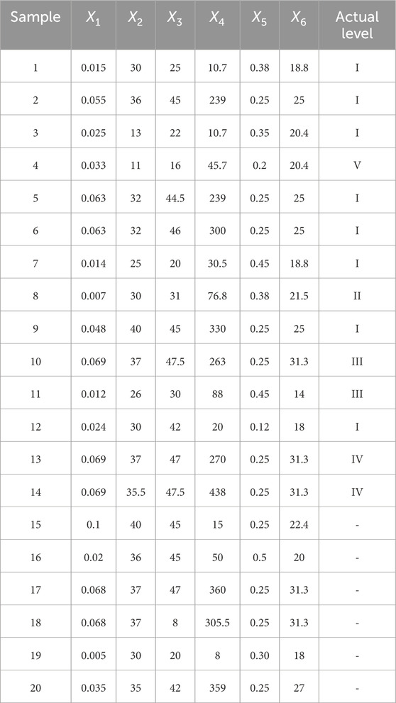
Table 1. The monitoring magnitude for the estimated sample.

In Table 1, the first 14 samples are selected as the training data, and the last six are chosen as the testing samples.

4.2 Standardizing the sample matrix

The sample data are standardized. Slope angle $\left(X_1\right)$, slope height $\left(X_2\right)$, and pore water pressure ratio $\left(X_3\right)$ belong to the benefit-type indicators; cohesion $\left(X_4\right)$, internal friction angle $\left(X_5\right)$, and natural unit weight $\left(X_6\right)$ belong to the cost-type indicators. They are standardized based on Equations 7, 11, respectively. The matrix $R$ is shown in Table 2.

Table 2

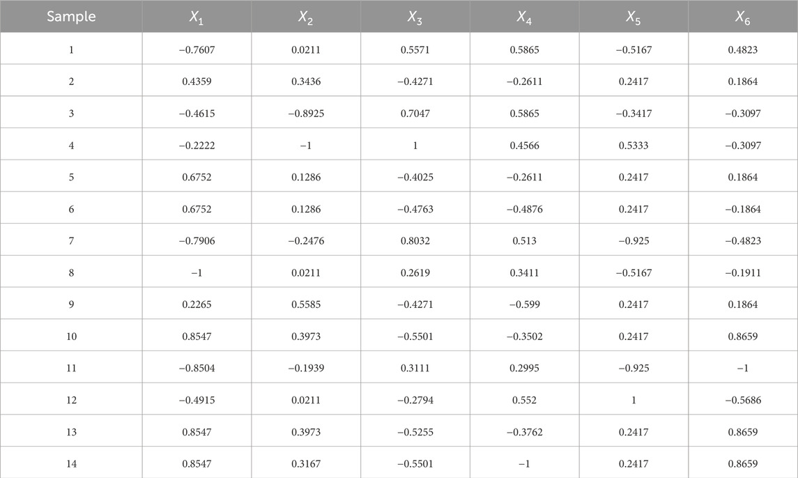
Table 2. Standardized sample matrix R.

4.3 Calculating weight coefficients

The correlation coefficient matrix is depicted in Table 3. It was calculated using SPSS software and in combination with Table 1.

Table 3

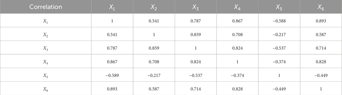
Table 3. The correlation coefficient matrix.

Table 4 uses Equations 1–5 to show the information entropy matrix of a separate index.

Table 4

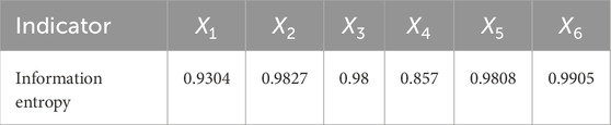
Table 4. The information entropy matrix.

Based on Equation 6, the weight coefficients can be obtained in Table 5.

Table 5

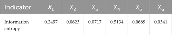
Table 5. The weight coefficient matrix.

4.4 Determining the relative target center distance

Relative target distance refers to the risk assessment index of a landslide. A larger magnitude indicates a higher risk level of the evaluated sample, and conversely, a lower risk level. According to Table 3 and Equations 12–14, the positive target center of the samples is determined as $r^{+}=\left(\begin{array}{cccccc}0.8547& 0.5585& 0.5501& 0.5865& 1& 1\end{array}\right)$, and the negative target center is $r^{-}=\left(\begin{array}{cccccc}-1& -1& -1& -0.599& -0.925& -0.8659\end{array}\right)$. The correlation coefficient matrix among evaluation indicators can be obtained based on the standardized sample indicator matrix R; it is shown in Table 4.

Table 4 shows that evaluation indicator $X_1$ has a strong correlation with $X_4$ and $X_6$; evaluation indicator $X_2$ has a strong correlation with $X_3$; $X_3$ has a strong correlation with $X_4$; $X_4$ has a strong correlation with $X_6$. To eliminate the impact caused by the correlation among evaluation indicators, the correlation coefficient matrix is introduced into the calculation of the relative target-heart distance.

The target center distance is calculated using Equations 15–17 and shown in Table 6.

Table 6

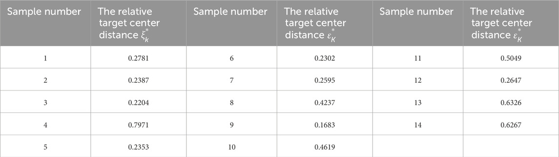
Table 6. The synthetic target center distance.

4.5 Determining the classification standard

Table 7 shows the relative target center distance standard based on Tables 5, 6, in combination with Equations 18, 19.

Table 7

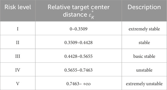
Table 7. The classification of risk level.

Its classification target is plotted in Figure 3.

Figure 3

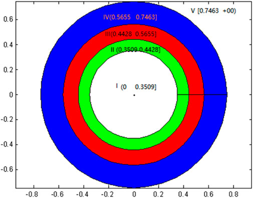
Figure 3. The classification target figure of slope risk grade.

4.6 Predicting the model

The last six groups of data in Table 1 are selected as the training sample. The risk level of samples can be determined based on the risk level classification, as shown in Table 7, and the relative target-center distances. The risk level obtained by the improved grey target model is consistent with the actual risk level. The actual risk level of this testing sample was determined based on geological data and exploration information. The comparison of results is presented in Table 8.

Table 8

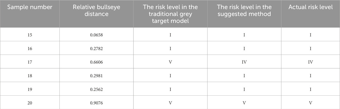
Table 8. The risk grade prediction of slope stability.

According to the comparative results of the assessment model in Table 8, conclusions can be drawn that the results obtained by the suggested method are entirely consistent with the actual risk level for six different samples. Its accuracy reaches 100% for the proposed approach. So, the conclusion demonstrates that it is feasible to estimate slope stability. Its accuracy is higher than the traditional grey target theory (Zhenhua et al., 2014) (the accuracy of the conventional theory is 83%). This is mainly because the traditional grey target model neglects the correlation between evaluation indicators during the evaluation process. This results in repeated computation of information and a reduction in the accuracy of evaluation results. For example, the positive correlation coefficient between the evaluation indicator $X_1$ and $X_4$ reaches 0.867. It can also be found in Table 8 that the risk levels of the slope stability from 15 to 20# samples are different; the risk level at slope sample #17 is IV, which means that slope sample #17 is unstable. Slope sample #20 is extremely unstable, so the corresponding consolidation measurement should be performed. For other samples, the slope is extremely stable; therefore, any measurements need not be taken.

5 Conclusion

1. An assignment method based on the characteristics of slope risk assessment was constructed based on the entropy weight theory. The correlation coefficient matrix was adopted to replace the covariance matrix in the Mahalanobis distance and was introduced into the traditional grey target model. A risk evaluation index system for the slope was established based on the root causes of slope prevention and management. The positive and negative target center distances using the Mahalanobis distance based on correlation coefficients are calculated, the relative target center distance is defined, and the slope risk levels are classified.

2. Considering the influence of the correlation among evaluation indicators, the correlation coefficient matrix is adopted to replace the covariance matrix in the Mahalanobis distance. It is introduced into the traditional grey target model, which can characterize the correlation among evaluation indicators, and therefore, the improved method enhances the accuracy of evaluation results. Meanwhile, the positive and negative ideal solutions in the TOPSIS model are introduced to define the positive and negative target centers. Thus, the drawback of the original grey target model is overcome, where only a single ideal optimal value is taken as the target core.

3. When the improved grey target model is applied to evaluate the practical slope risk level, the risk levels obtained from the enhanced model are consistent with the actual risk levels. From the perspective of considering indicator correlations, the validity and rationality of the improved grey target model in slope risk evaluation have been verified, indicating the enhanced grey target model’s feasibility in evaluating slope risk level.

4. The results obtained by the suggested method are entirely consistent with the actual risk level for six different samples. Its accuracy reaches 100% for the proposed approach. Its accuracy is higher than the accuracy of the conventional theory, which is 83%.

The suggested model predicts the slope stability accurately. In the future, due to its advantages, the model can be applied to environmental assessment, rock burst prediction, and surrounding rock quality evaluation, etc. Therefore, the theory will provide great application prospects.

Data availability statement

The original contributions presented in the study are included in the article/supplementary material; further inquiries can be directed to the corresponding author.

Author contributions

BZ: Writing – original draft, Formal Analysis, Funding acquisition. NL: Conceptualization, Writing – review and editing, Investigation. YC: Project administration, Supervision, Writing – review and editing. X-BG: Writing – original draft, Methodology.

Funding

The author(s) declare that financial support was received for the research and/or publication of this article. This work is supported by the Opening Project of Sichuan Province University Key Laboratory of Bridge Non-destruction Detecting and Engineering Computing (2022QYJ02, 2022QYY02), Key scientific research projects of colleges and universities in Henan province (23B560019).

Conflict of interest

The authors declare that the research was conducted in the absence of any commercial or financial relationships that could be construed as a potential conflict of interest.

Generative AI statement

The author(s) declare that no Generative AI was used in the creation of this manuscript.

Publisher’s note

All claims expressed in this article are solely those of the authors and do not necessarily represent those of their affiliated organizations, or those of the publisher, the editors and the reviewers. Any product that may be evaluated in this article, or claim that may be made by its manufacturer, is not guaranteed or endorsed by the publisher.

References

Botao, S., Zhang, Y., and Zhang, W. (2016). Material point strength reduction method for slope stability analysis. Chin. J. Geotechnical Eng. 38 (9), 1678–1684.

Google Scholar

Dong, J. (2016). Slope stability analysis based on improved particle swarm optimization algorithm. Anshan: University of Science and Technology Liaoning.

Google Scholar

Fang, Q., and Shang, L. (2019). Stability analysis of open-pit rock slope based on game theory-cloud model. J. Saf. Environ. 19 (1), 8–13.

Google Scholar

Gu, X. B., and Wu, Q. H. (2016). The application of nonordinary, state-based peridynamic theory on the damage process of the Advances in Materials Science and Engineering rock-like materials. Math. Problems Eng. 3 (8), 1–9.

Google Scholar

Gu, X. B., and Wu, Q. H. (2019). Seismic stability analysis of waterfront rock slopes using the modified pseudodynamic method. Geotech. Geol. Eng. 37 (3), 1743–1753. doi:10.1007/s10706-018-0718-1

CrossRef Full Text | Google Scholar

Gu, X. B., Ma, Y., Wu, Q. H., Ji, X. J., and Bai, H. (2021a). The risk assessment of landslide hazards in Shiwangmiao based on intuitionistic fuzzy sets-Topsis model. Nat. Hazards 111, 283–303. doi:10.1007/s11069-021-05053-5

CrossRef Full Text | Google Scholar

Gu, X. B., Shao, J. L., Wu, S. T., Wu, Q. H., and Bai, H. (2021b). The risk assessment of debris flow hazards in zhouqu based on the projection pursuit classification model. Geotechnical Geol. Eng. 8, 4–17.

Google Scholar

Gu, X. B., Wu, S. T., Ji, X. J., and Zhu, Y. H. (2021c). The risk assessment of debris flow hazards in Banshanmen gully based on the entropy weight normal cloud method. Adv. Civ. Eng. 2021, 8841310–8841311. doi:10.1155/2021/8841310

CrossRef Full Text | Google Scholar

Gu, X. B., Wang, L., and Wu, Q. H. (2022). The risk assessment of debris flow in the duba river watershed using intuitionistic fuzzy sets: TOPSIS model. Math. Problems Eng. 2022, 1–12. doi:10.1155/2022/2031907

CrossRef Full Text | Google Scholar

Gu, X.-B., Wu, Q.-H., and Ma, Y. (2025). Risk assessment of the rockburst intensity in a hydraulic tunnel using an intuitionistic fuzzy sets-TOPSIS model. Adv. Mater. Sci. Eng. 2022, 1–14. doi:10.1155/2022/4774978

CrossRef Full Text | Google Scholar

Jianye, Y. A. O., Zhang, S., and Hao, G. (2019). Slope stability evaluation based on set pair cloud model. Coal Geol. Explore 47 (1), 162–167.

Google Scholar

Jun, H. U., Dong, J., and Wang, K. (2016). Research on CPSO-BP model of slope stability. Rock Soil Mech. 37 (S1), 577–582.

Google Scholar

Liu, G. (2014). Application of set pair model of game theory comprehensive weighting in risk analysis of rock and soil slope stability[D]. Hengyang, Hunan, China: University of South China.

Google Scholar

Shou, Y., Guo, L., and Zhou, X. (2024). Development of the rolling extrusion rock bolt with constant resistance and large deformation. Deep Resour. Eng. 1 (1), 100004. doi:10.1016/j.deepre.2024.100004

CrossRef Full Text | Google Scholar

Wang, B., Xiating, F., and Pan, P. (2017). Application research of material point method in slope stability evaluation. Chin. J. Rock Mech. Eng. 36 (9), 2 146–2 155.

Google Scholar

Wang, H., Zhang, Y., and Haiyue, M. A. (2019). Comprehensive evaluation of open-pit mine slope stability based on GA-PP model. Min. Res. Dev. 39 (2), 30–33.

Google Scholar

Xue-bin, , and Chang-liang, P. A. N. (2007). Rock burst prediction method based on grey whitenization weight function cluster theory. J. Hunan Univ. Nat. Sci. 34 (8), 16–20.

Google Scholar

Yang, W., Dong, Y., and Xie, Q. (2018). Slope risk assessment method based on cloud model and its application. J. Huazhong Univ. Sci. Technol. 46 (4), 30–34.

Google Scholar

Yongqiang, J., Huaizhi, S., and Ziyang, L. (2007). Slope stability projection pursuit clustering analysis based on harmonic search. J. Hydraulic Eng. 38 (S1), 682–686.

Google Scholar

Yuansong, L., Chen, W., and Xinping, L. I. (2013). Slope stability evaluation method based on fuzzy neural network. J. Wuhan Univ. Technol. 35 (1), 113–118.

Google Scholar

Zhang, J., and Yang, T. (2018). Study of a roof water inrush prediction model in shallow seam mining based on an analytic hierarchy process using a grey relational analysis method. Arab. J. Geosci. 11, 153. doi:10.1007/s12517-018-3498-2

CrossRef Full Text | Google Scholar

Zhao, Y., and Liu, H. (2012). An elastic stress–strain relationship for porous rock under anisotropic stress conditions. Rock Mech. Rock Eng. 45, 389–399. doi:10.1007/s00603-011-0193-y

CrossRef Full Text | Google Scholar

Zhao, Y., He, P., Zhang, Y., and Wang, C. (2019a). A new criterion for a toughness-dominated hydraulic fracture crossing a natural frictional interface. Rock Mech. Rock Eng. 52, 2617–2629. doi:10.1007/s00603-018-1683-y

CrossRef Full Text | Google Scholar

Zhao, Y., Wang, C., Zhang, Y., and Liu, Q. (2019b). Experimental study of adsorption effects on shale permeability. Nat. Resour. Res. 28, 1575–1586. doi:10.1007/s11053-019-09476-7

CrossRef Full Text | Google Scholar

Zhao, Y., Bi, J., Wang, C., and Liu, P. (2021). Effect of unloading rate on the mechanical behavior and fracture characteristics of sandstones under complex triaxial stress conditions. Rock Mech. Rock Eng. 54, 4851–4866. doi:10.1007/s00603-021-02515-x

CrossRef Full Text | Google Scholar

Zhao, Yu, Wang, C., Lin, N., Zhao, H., and Bi, J. (2022a). Pore and fracture development in coal under stress conditions based on nuclear magnetic resonance and fractal theory. Fuel 309, 122112. doi:10.1016/j.fuel.2021.122112

CrossRef Full Text | Google Scholar

Zhao, Y., Zhang, Y., Wang, C., and Liu, Q. (2022b). Hydraulic fracturing characteristics and evaluation of fracturing effectiveness under different anisotropic angles and injection rates: an experimental investigation in absence of confining pressure. J. Nat. Gas Sci. Eng. 97, 104343. doi:10.1016/j.jngse.2021.104343

CrossRef Full Text | Google Scholar

Zhao, Y., Wang, C., and Bi, J. (2023). Analysis of fractured rock permeability evolution under unloading conditions by the model of elastoplastic contact between rough surfaces. Rock Mech. Rock Eng. 53, 5795–5808. doi:10.1007/s00603-020-02224-x

CrossRef Full Text | Google Scholar

Zhenhua, X., Shasha, L., and Zhang, X. (2014). Early warning method for instability of open pit slope based on RBF neural network. Metal. Mine 32 (9), 7–10.

Google Scholar

Zhou, X. P., Zhang, Y. X., Ha, Q. L., and Zhu, K. S. (2008). Micromechanical modelling of the complete stress–strain relationship for crack weakened rock subjected to compressive loading. Rock Mech. Rock Eng. 41 (5), 747–769. doi:10.1007/s00603-007-0130-2

CrossRef Full Text | Google Scholar

Zhou, X. P., Pan, X. K., and Cheng, H. (2021). The nonlinear creep behaviors of sandstone under the different confining pressures based on NMR Technology. Rock Mech. Rock Eng. 54 (9), 4889–4904. doi:10.1007/s00603-021-02557-1

CrossRef Full Text | Google Scholar