 Siyi Qu1
 Shengping Wang1*
 Fan Zhou1Wenxin Li1Desheng Cai1Zhiqiang Zhang2
 Peter Strauss3Kewen Wang1Yiyao Liu1
- 1College of Hydraulic and Hydro-Power Engineering, North China Electric Power University, Beijing, China
- 2College of Soil and Water Conservation, Beijing Forestry University, Beijing, China
- 3Institute for Land and Water Management Research, Federal Agency for Water Management, Petzenkirchen, Austria
Introduction: Assessing ecosystem health and understanding its potential environmental controls are critically important for effective revegetation of mountainous areas where multiple agents may constrain ecosystem health and ecosystem usually fragiled accordingly.
Methods: We applied the VOR framework (vigor–organization–resilience model) to assess ecosystem health of a meso-scale mountainous watershed of northern China (Xiaoluan River watershed), and quantified environmental controls by integrating Ordinary Least Squares (OLS), Geographically Weighted Regression (GWR) and Multiscale Geographically Weighted Regression (MGWR) techniques.
Results: With the proceeding of revegetation, ecosystem health of the watershed showed a slight improvement over 2006-2020 (p > 0.05), EHI (ecosystem health index) varied from 0.49 to 0.57, and the ecosystem resilience (ER) remained relatively low, with the mean ER over the years being only 0.19. Additionally, Moran's I showed strong spatially positive autocorrelations, especially for the plant functional types (PFTs) of NETT (Needleleaf evergreen tree, temperate) and BDTT (Broadleaf deciduous tree, temperate), indicative of a proneness to abrupt transition in case of an environmental perturbation. Both OLS and GWR (including MGWR) models suggested that thermal stress and water stress both are primary constraints on the ecosystem health of the watershed, and at seasonal scales, their controls alter by season, with T dominating in the beginning of growing season, whilst P dominates in growing season, well characterizing the major process controlling EHI of mountainous watersheds in transitional zone of northern China.
Discussion: Given intensified climate change and widespread revegetation, greater caution should be exercised when implementing large-scale afforestation in the region to avoid potential ecosystem collapse under environmental disturbances. Strategies to enhance resilience and adapt vegetation types to local hydrothermal conditions are recommended.
1 Introduction
Mountains are commonly one of the most fragile ecosystems on earth, being easily affected by global environmental change (Chu et al., 2019; Thakur et al., 2021; Zhai et al., 2023). Due to global climate change and the increasing population, mountainous areas are widely considered in various research studies of global environmental change and ecological protection and restoration (Wang et al., 2022). This is also true for northern China, where the areas are often expected to provide ecosystem services, such as supplying water resources to the downstream areas and offering green shelters to the surrounding areas (Li et al., 2012; Shao et al., 2023). However, due to limited rainfall availability and poor soil quality, the areas are often constrained by the unfavorable environment, especially with respect to ecological development (Shao et al., 2023). In order to restore and maintain the ecological environment of these areas, the Chinese government has launched several restoration programs over the years, such as the “Grain for Green project” and the “Three North Shelterbelt Forest Program (TNSFP).” The TNSFP is reported to have increased forest coverage from 5.05% in 1978 to 13.84% in 2024 (Zhai et al., 2023).
Several studies have been carried out to understand the change in ecological quality of the region due to revegetation (Duan et al., 2011; Jiang et al., 2021; Zhang and Zhang, 2024), and various frameworks and/or approaches were used. In addition to directly assessing the trend of vegetation variations using individual indices such as normalized difference vegetation index (NDVI) (Martínez and Gilabert, 2009; Ibrahim et al., 2015), vegetation drought is also widely considered in the relevant research studies. For example, Cunha et al. (2015) assessed vegetation drought in the semiarid region of Brazil and suggested the vegetation supply water index, which is closely related to rainfall and soil moisture. Won and Kim (2023) introduced the EDCI-veg index to monitor the impact of meteorological drought on vegetation, effectively exploring how land covers respond to various drought conditions. Unlike the above analysis, which is dedicated to revealing one aspect of vegetation quality, the classical ecosystem vigor–organization–resilience (VOR) assessment framework focuses on measuring ecosystem integrity and natural ecosystem quality, and it has been successfully employed to evaluate ecosystem health (Shen et al., 2021; Yushanjiang et al., 2021; Bao et al., 2022; Ma et al., 2022; Yin et al., 2024). Peng et al. (2017) used the traditional VOR model to calculate the index of regional ecosystem physical health and introduced the coefficient of spatial neighborhood effect, generating the index of integrated ecosystem health in Lijiang, China. On the basis of the traditional VOR framework, Pan et al. (2021) proposed an improved method that considers both ecological integrity and ecosystem services demand and applied their new method in the Yangtze River economic belt in China. Bao et al. (2022) introduced more metrics into the VOR framework, aiming to optimize and improve the VOR application. Although various frameworks provide optional approaches for examining ecosystem quality and ecological health, most have been limited to depicting vegetation dynamics and vegetation health, while the dominant factors controlling ecosystem health in these areas appear to be rarely investigated.
In the study conducted by Ge et al. (2022), the authors used the Geodetector model to examine the effects of various factors on ecosystem health. The results show that the state of natural balance maintenance in the Chinese land system, influenced by social factors, is the main factor affecting ecosystem health, along with interactions among various factors. Considering the spatio-temporal variability in ecosystem health and its influencing factors, Li K. M. et al. (2024) and Na et al. (2023) investigated the spatial relationships between ecosystem health and its factors concerning climate, socioeconomic status, and natural resource endowment at the county level based on a geographically weighted regression (GWR) model. Meanwhile, Ouyang et al. (2024) integrated the extreme gradient boosting (XGBoost) model and Shapley additive explanation (SHAP) model to assess the impact of urbanization level and meteorological and vegetation factors on ecological health. These methods not only provide an explicit depiction of the impacts of the driving factors but also offer a deeper understanding of the possible mechanisms.
In our analysis, the Xiaoluan River watershed is located in the transitional zone between the Inner Mongolia Plateau and the North China Plain, featuring plateau characteristics in the upstream region and a typical mountainous and hilly region in the middle and downstream areas. As one of the typical areas serving as both an ecological barrier and a nature reserve, its ecological health directly affects the ecological security of downstream areas, especially in terms of maintaining biodiversity and conserving soil and water, and holds strategic significance for resource supply and ecological protection, particularly for regions such as Beijing. With ongoing revegetation efforts and global climate warming, it is necessary to understand the development of ecosystem health in the region and the dominant factors influencing it, which would contribute to the management of the natural watershed, ensuring healthy and sustainable development of the regional ecosystem.
The purpose of this study is to assess the change in ecosystem health of the natural watershed using the traditional VOR framework and uncover the potential environmental controls that mediate the variations in ecosystem health of the region. Specifically, we aimed to i) evaluate the spatial and temporal variations of ecosystem health of the watershed, ii) diagnose the clustering pattern of the ecological health, and iii) identify the dominant constraints of ecosystem health with respect to climatic, topographic, and pedological aspects.
2 Methods
2.1 Study area
The Xiaoluan River watershed is located in the transitional zone between the Inner Mongolia Plateau and the mountains of northern Hebei (Figure 1). It is situated between 116°30′ E–117°30′ E and 41°30′ N–42°30′ N, with an altitude of 768 m–1,904 m. The drainage area of the watershed is 1,980 km2, and the mean annual temperature and precipitation during the study period are 3.54 °C ± 1.77 °C and 414.64 mm ± 15.32 mm, respectively. This area is a typical transition zone between forests and grasslands. The main land use types are mainly forest and grassland, with forests mainly distributed in the lower reaches of the watershed and grassland in the middle and upper reaches.

Figure 1. Geographical location of the Xiaoluan River watershed.
Soils in the middle and upper reaches are mainly gravelly and sandy texture in texture, while the middle and lower reaches contain more medium-textured soils. The watershed is located in a Quaternary accumulation zone, characterized predominantly by Quaternary wind-blown deposits and sediment cover (Houyun et al., 2020).
2.2 Data availability
We obtained monthly precipitation and temperature data from 2006 to 2020 (Table 1), which were used to calculate the annual average precipitation and temperature variability; these variables were then included in the regression model to investigate their potential influence on ecosystem health. Spatial grid vegetation datasets for the same time period, including the enhanced vegetation index (EVI) and NDVI, were acquired from LAADS DAAC. Land surface temperature (LST) was from Landsat 5, Landsat 7, and Landsat 8 series remote-sensing images and was synthesized on the GEE platform. Land-use information was from the Earth System Science Data. Considering the discrepancy in the resolution of various sources, the inverse distance weighting (IDW) method was used to interpolate the dataset into a uniform grid of 250 m × 250 m. The maximum distance was set to the diagonal length of the analysis extent, and the search radius type was adjusted based on the number of points, while all other parameters were kept at their default settings in ArcGIS 10.2. These datasets were all used in the VOR framework analysis. Additionally, in order to explore the potential topographic and pedological controls on ecosystem health, datasets on soil properties and digital elevation models (DEMs) were also included in the construction of the regression models.
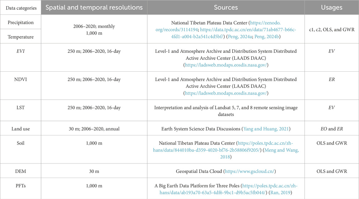
Table 1. Data sources and their spatiotemporal resolution.
2.3 VOR framework for ecosystem health assessment
The classic VOR framework developed by Costanza et al. (1997) is widely used for assessing ecosystem health (Ma et al., 2022), which combines ecosystem vigor (EV), ecosystem organizational capacity (EO), and ecosystem resilience (ER) into the EHI (Equation 1).
EV, EO, and ER all range from 0 to 1, with 0 indicating a poor condition and 1 indicating a good condition.
2.3.1 EV
EV is the most visual component of the VOR model, representing ecosystem health. Various approaches were often employed to quantify this component (e.g., NDVI (Peng et al., 2017), NPP (Pan et al., 2021), GPP (Yushanjiang et al., 2021), or a combination of metrics (Bao et al., 2022)). Considering that the combination of the vegetation condition index and thermal condition index is a good indicator of soil moisture content, along with reflecting the condition of vegetation and the health of the ecosystem (Cunha et al., 2015), both EVI and LST were included in our case to characterize EV. EV is calculated using Equation 2 as follows:
where α is a weight parameter that is usually set as α = 0.5 (Bento et al., 2018).
2.3.2 EO
EO refers to the structural stability of an ecosystem (see Equation 3), including the landscape connectivity (LC), landscape heterogeneity (LH), and connectivity of essential patches (IC) (Abbas et al., 2022). Following the method of Bao et al. (2022), we estimated EO according to Equation 3, in which LC, LH, and IC were estimated using Fragstats 4.2:
2.3.3 ER
ER is defined by the ecosystem’s resistance to external disturbance and its capacity for recovery (see Equation 4) (López et al., 2013; Yushanjiang et al., 2021):
Here,
2.4 Spatial autocorrelation analysis
Moran’s I is usually used to investigate the spatial autocorrelation for understanding the spatial distribution pattern of variables and the clustering status of an ecosystem (Song et al., 2024). Both Shi et al. (2022) and Fu et al. (2014) used Moran’s I to quantify the spatial correlations of the investigated variables in their research areas. However, Wu et al. (2024) and Song et al. (2024) used Moran’s I to identify spatial clustering in the ecosystems of the investigated areas. In our analysis, we attempted to use global Moran’s I (see Equations 5–7) to identify the spatial correlation of ecosystem health and understand the resilience of ecosystem health in the Xiaoluan River watershed (Wu et al., 2024).
Here,
Considering that when global Moran’s I is 1, there may not necessarily be local spatial clustering, local Moran’s I (see Equations 8–10) was also estimated in our analysis to reveal the difference in spatial dependence of ecosystem health between areas. The local Moran’s I can reveal the distribution of high and low EHI values within a region, thereby screening out statistically significant spatial clusters of high values (hot spots), low values (cold spots), and spatial outliers (Zhang et al., 2008; Fu et al., 2014). For instance, HH is representative of the areas with high EHI surrounded by neighboring areas of high EHI; LL is representative of the areas with low EHI surrounded by neighboring areas with low EHI; LH is representative of the areas with low EHI surrounded by neighboring areas with high EHI; and HL is representative of the areas with high EHI surrounded by neighboring areas with low EHI. The last two clustering types represent the negative autocorrelations of the EHI. Zhou et al. (2022) elucidated the patterns of spatial autocorrelation of ecological health using local Moran’s I. In this study, we also tried to use local Moran’s I to identify local spatial clustering patterns and spatial outliers (Harries, 2006; Fu et al., 2014).
Here,
2.5 Potential variables affecting variance of ecosystem health
The spatial and temporal variance of ecosystem health is often the result of multiple driving processes. In addition to the influence of climatic variables (Cartwright et al., 2020; Jiang et al., 2021; Teng et al., 2023), various other factors have also shown their importance in different ecological processes. For example, soil moisture is a key variable in the soil–plant–atmosphere system (Wang et al., 2018), while the topographic wetness index (TWI) is moderately well-correlated with observed soil moisture patterns (Buchanan et al., 2014) and is often used as a proxy for soil moisture (Kopecký et al., 2021). The interaction between topographic and pedological processes is usually found to exert a dominant influence on the EHI (Cartwright et al., 2020; Huang et al., 2023; Li M. et al., 2023; Bandak et al., 2024). In addition, human activities such as socio-economic development and policies also play a role in mediating EHI (Ge et al., 2022; Li K. M. et al., 2024). Given that the study area is a natural watershed with minimal human interference, only climatic, soil, and topographic variables were included in the analysis to explore their potential influence on variations in the EHI (Table 2). Both ordinary least squares (OLS) and GWR regression techniques were utilized to examine the relationships between ecosystem health and the potential affecting variables. All the variables were standardized to eliminate the impacts of magnitude, dimension, and positive and negative orientations.

Table 2. Indicators of factors influencing ecosystem health.
2.5.1 Global linear regression
The OLS technique can screen identify independent variables that have a significant impact on the EHI from the independent variables, providing a simple and effective method for revealing the influence of potential predictors on the response variable (Yu and Peng, 2019; Gao et al., 2022; Kalwa et al., 2023). Several studies have successfully applied OLS models to analyze the effects of the various morphological variables on LST from a global perspective (He et al., 2019; Gao et al., 2022; Khalid et al., 2024). Assuming that a linear relationship exists between the EHI and the potential explanatory variables, we established annual global linear regression models for the watershed using the OLS technique. The variables related to soil properties, topography, and climate were considered the explanatory variables, and EHI was the dependent variable. Six variables including soil bulk density (SBD), upper soil silt content (USI), upper soil clay content (UCL), deep soil silt content (DSI), deep soil sand content (DSA), and deep soil pH value (DpH) were excluded from the OLS models to control the variance inflation factor (VIF) within a reasonable range, and the remaining variables that were retained in the OLS models were upper soil pH value (UpH), USA, TWI, relief degree of land surface (RDLS), T, P, deep soil clay content (DCL), and available water capacity (AWC), with most of their VIF values being lower than 10, except for USA and DCL (being 12.90 and 11.96, respectively). In order to understand the possible differences in environmental controls on the EHI among different plant functional types (PFTs), separate regression models were established for each PFT.
2.5.2 Geographically weighted regression model
In contrast to OLS models, which may overlook spatially dependent and heterogeneous relationships among variables, the GWR model is usually employed to account for spatial dependence and heterogeneity in the factors influencing the EHI (Xu and Lin, 2017; Shi et al., 2022). It is an effective method for detecting spatial non-stationarity between the explanatory and dependent variables (Brunsdon et al., 2010; Zhu et al., 2020). The essence of GWR modeling is to establish multiple regression models within the investigated areas by accounting for spatially varied weights for the variables (see Equation 11) (Xu and Lin, 2017; Yu and Peng, 2019; Khalid et al., 2024). Xu and Lin (2017) successfully applied the GWR model to quantify the relationship between the carbon sink of cropland and its influencing factors at various scales. Li M. et al. (2024) investigated the spatially varied effects of potential variables on ecological risk using the GWR model.
Here,
We first established GWR models for the grids of the watershed. The kernel type used was the bi-square kernel, with an adaptive bandwidth determined using the golden section search method. The optimal bandwidth represents the spatial scale at which processes influencing the dependent variable operate. Considering that various processes may not operate at the same scale, in contrast to the assumption of the classical GWR modeling approach (Fotheringham et al., 2017), multiscale geographically weighted regression (MGWR) models were also employed. The influence of explanatory variables on the EHI was compared between the GWR and MGWR models.
The performance of both the GWR and OLS models was evaluated using the −2 log-likelihood (−2LL), residual sum of squares (RSS), and Akaike’s information criterion corrected (AICc) methods. A smaller RSS means a better fit, as do smaller AICc and −2LL. Conversely, a higher adjusted R2 indicates a better fit.
In order to examine whether the EHI of different PFTs differed and how environmental controls varied across PFTs, in addition to the analysis for the entire watershed, we also carried out a stratified analysis with respect to EHI estimation and GWR modeling using the five plant function types of the watershed, namely, needleleaf evergreen tree, temperate (NETT); broadleaf deciduous tree, temperate (BDTT); broadleaf deciduous tree, boreal (BDTB); broadleaf deciduous shrub, temperate (BDST); and C3 grass (C3).
3 Results
3.1 Spatial and temporal variance of ecosystem health
3.1.1 EV
Unexpectedly, the EV of the watershed showed a slightly decreasing trend (p > 0.05) from 2006 to 2020, probably due to the significant (p < 0.05) decrease in the EVI. The average annual EV of the watershed was 0.50. Governed by the land uses, EV displayed a spatially varied distribution. The grassland located mainly in the northwest area generally had lower EV values with higher standard deviations, while the forest land generally showed relatively higher EV values and lower standard deviations (Figure 2). Stratifying the EV values by PFTs, the plant type of BDTT had the highest EV, followed by BDTB, NETT, BDST, and C3, with their EV values being 0.55, 0.57, 0.55, 0.53, and 0.48, respectively (Figure 3A). Except for NETT and BDTB, there were significant differences in EV between the other types.
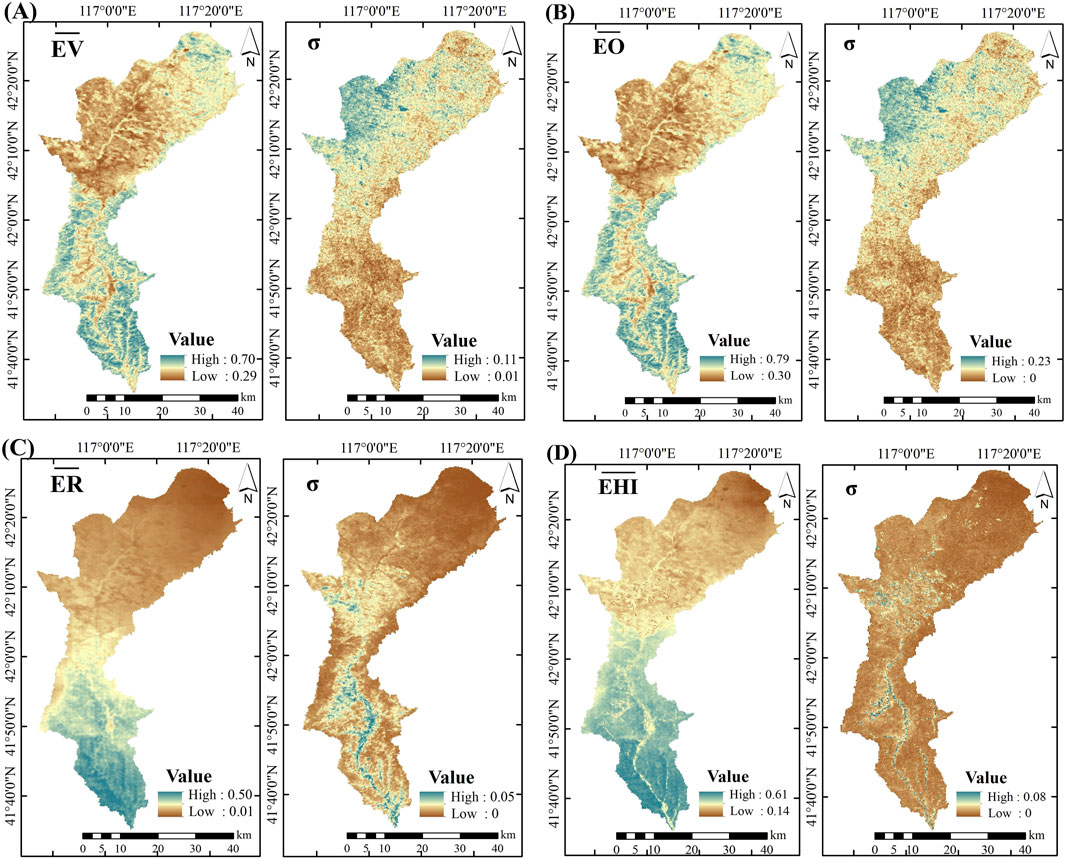
Figure 2. Spatial distribution of the average annual (A) EV, (B) EO, (C) ER, and (D) EHI over 2006–2020.
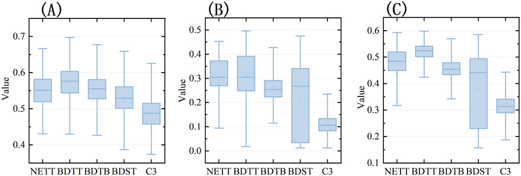
Figure 3. Box plots for (A) EV, (B) ER, and (C) EHI for the five PFTs. The box represents the interquartile range (IQR) of EV, EO, ER, and EHI; the whiskers refer to the range within the first and third quartiles; the line inside represents the median; the hollow square indicates the mean value of the data.
3.1.2 EO
The mean annual EO of the watershed was 0.65, suggesting a moderate landscape heterogeneity and connectivity of the watershed. EO did not show an obvious spatial pattern across the whole watershed (Figure 2). Except for the areas along the river network, which were mainly cropland, the remaining areas displayed higher EO values. No significant difference was found in EO values among different PFTs.
3.1.3 ER
The mean annual ER of the watershed was 0.19, with an insignificant increasing trend (p > 0.05) from 2006 to 2020. ER also exhibited an obvious spatially divergent distribution, with lower values in the upper half of the watershed and higher values in the lower half (Figure 2). This pattern was assumed to be influenced by both land use type and temperature. ER showed a relatively stable state over the years across almost the whole watershed, with the mean SD values of 0.01, which is indicative of a very constant resilience level (Figure 3). When the five plant types were examined, both BDTT and NETT exhibited stronger resistance, with their ER values at 0.31 ± 0.09 and 0.28 ± 0.13, respectively; these were followed by BDTB, BDST, and C3, with ER values of 0.26 ± 0.08, 0.21 ± 0.15, and 0.12 ± 0.07, respectively (Figure 3B). There is a significant (p < 0.05) difference in ER between the five PFTs.
3.1.4 EHI
The spatially averaged annual EHI of the watershed varied ranged 0.36 to 0.39 from 2006 to 2020, showing no significant (p > 0.05) increasing trend over the period. Governed by EV and ER, the EHI also showed a spatially varied distribution. The lower portion of the watershed usually had higher EHI values, while the upper portion of the area had lower EHI values (Figure 2). The SD values of the EHI during the investigated time period were lower across the watershed, indicating a relatively stable level with respect to the ecosystem health over the years.
Among the five dominant PFTs, the vegetation type with the highest EHI is still BDTT (EHI being 0.52 ± 0.03), followed by BDTB, NETT, BDST, and C3 (EHI being 0.45 ± 0.06, 0.44 ± 0.12, 0.38 ± 0.13, and 0.32 ± 0.06, respectively). There are significant (p < 0.05) differences in the EHI among the five PFTs. It is worth noting that the EHI in the upstream areas of the watershed was generally lower than that in the downstream areas, even for the same PFT. One of the possible reasons is that the watershed exhibited distinct climatic conditions between the upstream and downstream areas, with the vegetation being greatly influenced by the availability of thermal resources. As the elevation increased in upstream areas, temperature greatly decreased, thereby constraining vegetation productivity accordingly. A detailed explanation is provided in the discussion section.
3.2 Spatial autocorrelation of ecosystem health
Global Moran’s I analysis suggests that the distribution of ecosystem health of the Xiaoluan River watershed is not randomly developed. The EHI value showed a strong spatially positive autocorrelation, with a mean global Moran’s I of 0.92 ± 0.01, and no significant trend was detected from 2006 to 2020.
Among the five PFTs, BDTT had the highest EHI, with the mean annual global Moran’s I being 0.55, and it was significantly lower than those of the others (0.96 for NETT, 0.87 for BDTB, 0.97 for BDST, and 0.96 for C3). The relatively lower Moran’s I value for BDTT suggests weaker spatial dependence on surrounding areas with respect to its ecosystem health. This is mainly because the distribution of BDTT in the watershed is much more concentrated (Ran, 2019) and the EHI varies considerably within these concentrated areas; in contrast, the other PFTs are more widely dispersed across the watershed, with smoother EHI variations, thus resulting in stronger spatial autocorrelation.
In line with global Moran’s I, local Moran’s I suggests that the ecosystem health of the watershed exhibited strong spatially positive autocorrelations (Figure 4) as both the HH and LL areas accounted for 26.0% and 17.8% of the whole watershed. The mean local Moran’s I for the HH clustering was 1.90, and it was highly concentrated in the southern part and partially in the northeastern part of the watershed, with the land use type mainly being forest (Figure 4B). Meanwhile, the LL clustering had a mean local Moran’s I of 1.66 and was primarily distributed in the northern part of the watershed and along the river network (Figure 4C), where the dominant land use type was agricultural land. HL areas have relatively good local ecosystem health, but their surrounding areas are comparatively poor. LH areas have relatively poor local ecosystem health, but their surrounding areas are comparatively good. Both occur infrequently and are sporadically distributed in certain regions during specific years (Figures 4A, D).
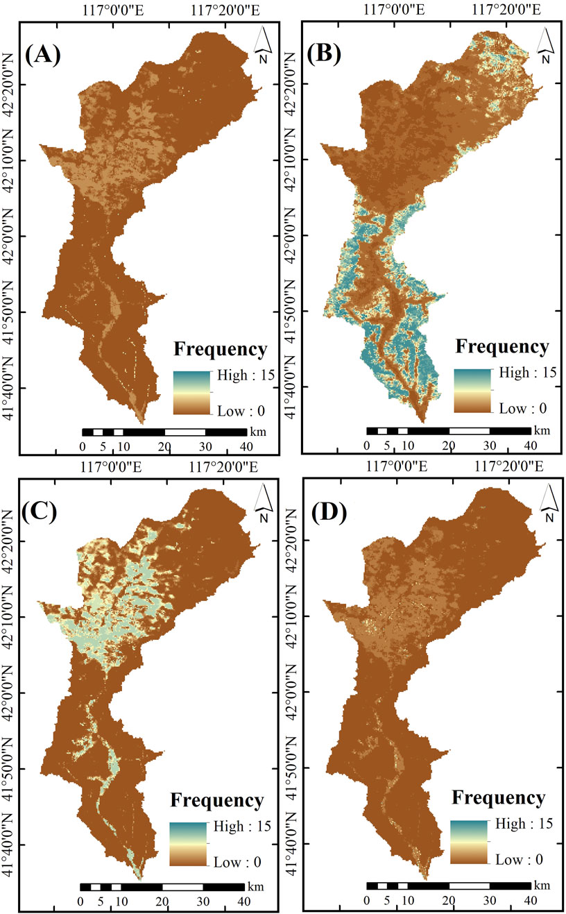
Figure 4. Frequency for the occurrence of each cell identified with either hot or cold spots from 2006 to 2020. (A) HL, (B) HH, (C) LL, and (D) LH. The values of the frequency were estimated using the number of years exhibited with either hot or cold spots for each cell divided by the total number of years.
As shown in Table 3, stratifying the clustering results by the PFTs indicated strong spatial autocorrelation in ecosystem health for both NETT and BDTT. HH clustering accounted for 75% and 97% of their corresponding total areas, with the mean local Moran’s I values of 1.89 and 2.47 for NETT and BDTT, respectively. BDST also displayed a spatially positive correlation, with the mean local Moran’s I values of 1.81 and 2.61 for HH and LL clusters, accounting for 45% and 37% of the areas, respectively. BDTB showed a different spatial clustering pattern. In addition to the HH clustering type, nearly half of the areas (47%) showed no significant spatial relationship, suggesting a lower degree of spatial dependence in ecosystem health across those areas.
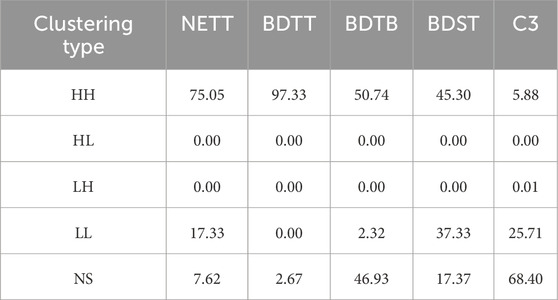
Table 3. Percentage of the area (%) occupied by different clustering types for each PFT. The values were estimated using the areas of each clustering type (i.e., HH, LL, HL, and LH) divided by the total areas of the corresponding PFT (NS means not significant).
3.3 Potential environmental controls on the EHI
3.3.1 OLS models
Except for variables DO and UO, the other variables, including RDLS, TWI, AWC, USA, UpH, DCL, T, and P, had significant impacts (p < 0.05) on ecosystem health. T had the most prominent positive control on the EHI, and the mean regression coefficient was as high as 0.70 ± 0.04 (Figure 5). This is mainly because the area is characterized by a long winter season, commonly ranging from the end of October to the middle of April, with a mean annual temperature of 3.54 °C ± 1.77 °C, and the recorded minimum air temperature over the period of 2006–2020 being −10.64 °C only. The long-term available energy, therefore, predominantly controlled the recovery of ecosystem health of the watershed. P also showed a positive control on the EHI of the watershed, with the mean annual regression coefficient of 0.13 ± 0.03, suggesting its dominant control on the ecosystem health of the areas. Both soil variables, USA and DCL, exhibited a positive and fair share of controls on the EHI, with their regression coefficients being 0.18 ± 0.03 and 0.11 ± 0.01, respectively. Unexpectedly, both TWI and AWC, which are commonly representative of soil wetness, showed weaker control over the EHI, with the mean annual regression coefficients even being negative, i.e., −0.06 ± 0.01 and −0.07 ± 0.02, respectively. We suggest that the lack of positive correlations between the EHI and these two variables may be partially attributed to limited data recorded for AWC of the areas in the HSWD dataset and the inability of the TWI to differentiate soil wetness at the spatial scale of the investigated watershed. A detailed explanation is provided in the discussion section.
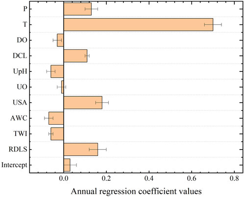
Figure 5. Regression coefficients of the explanatory variables for estimating annual EHI using the OLS technique. The bar is the mean value of the estimated coefficients during 2006–2020, and the whisker denotes the standard deviation of the coefficient estimations.
3.3.2 GWR models
Compared with OLS models, the RSS values of the GWR models reduced by 24.4%, the –2LL value reduced by 12.1%, and the AICc value reduced by 11.3%, while the adjusted R2 values were enhanced by 3.62% (Figure 6). The improved performance of the GWR models suggests that the GWR approach is more effective in capturing both the environmental controls on the EHI and its locally specific variations across the study area.
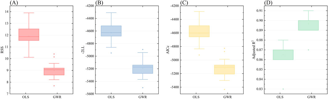
Figure 6. The evaluation results of OLS and GWR models using (A) RSS, (B) -2LL, (C) AICc, and (D) adjusted R2.
The local regression coefficients (LRCs) of the explanatory variables from the GWR models are shown in Figure 7. The greater the absolute value, the stronger the variable’s control over the EHI. In line with the results of the OLS models, T showed a dominant control on the EHI across the watershed, with the LRC values in the northern area being as high as 0.94 (Figure 7g). P also played an important role in affecting EHI variation, but its magnitude was less than that of T, with the spatially averaged LRC value across the areas being 0.15 ± 0.05 (Figure 7h).
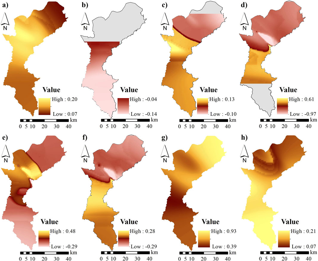
Figure 7. Spatially distributed LRC values for (a) RDLS, (b) TWI, (c) AWC, (d) USA, (e) UpH, (f) DCL, (g) T, and (h) P derived from the GWR models over 2006–2020.
Primarily due to the spatially divergent distribution of soil texture of the watershed (Figure 8), the variables of soil properties, including USA, DCL, and UpH, exhibited moderate but spatially varied controls on the EHI. For example, USA had negative effects on the EHI in the upstream areas of the watershed, while it showed positive effects in the middle-stream areas (Figure 7d), with a spatially averaged LRC of −0.22 ± 0.23. Both UpH (Figure 7e) and DCL (Figure 7f) also showed spatially variable influences on the EHI, with average LRC values of 0.01 ± 0.11 and −0.04 ± 0.12, respectively.

Figure 8. Spatial distribution of (A) USA (B) DCL, and (C) UpH in the Xiaoluan River watershed.
The effects of the topography variable (i.e., RDLS) on the EHI were comparable to those of soil variables (see Figure 7a), with a spatially averaged LRC value of 0.13 ± 0.04. Higher LRC values were predominantly observed in the central area, mainly characterized by a flat terrain and covered with C3. In contrast, in other areas commonly covered with arboreal forest, the LRC values were relatively lower regardless of RDLS, indicating weaker topographic control on the EHI of arboreal forests in the region.
Both TWI and AWC, usually used as proxies for soil moisture (Bertoldi et al., 2014), have shown moderate and slight controls on the EHI, respectively (Figures 7b, c), with their spatially averaged LRC values of −0.00 ± 0.08 for TWI and −0.012 ± 0.04 for AWC. We suggest that the negative influence of the TWI on the EHI is mainly due to the relatively high clay content (29%) in the watershed’s soil, especially in the downstream areas (Figure 8b), resulting in unfavorable soil moisture conditions for vegetation growth in depressions.
The results of MGWR were generally consistent with those of GWR. Specifically, the climatic variable T presented a dominant control on ecosystem health in the study area, with average LRC values from the GWR models as high as 0.69 ± 0.20, and in comparison, the LRC value for P was 0.18 ± 0.01 (Figure 9). The variables, TWI and AWC, representing soil moisture condition, displayed moderate and slight controls on the EHI, with their averaged LRC values being −0.08 ± 0.02 and −0.03 ± 0.00, respectively. The topography variable of RDLS has shown moderate effects on the EHI, with the LRC value being 0.06 ± 0.01. As for the soil variable, except for UpH, both DCL and USA showed positive effects on the EHI, which were significantly distinct from those of GWR. We mainly ascribe the difference to the scales of the GWR and MGWR models estimated. In other words, the MGWR technique used a larger bandwidth to establish models than the GWR did in our case.
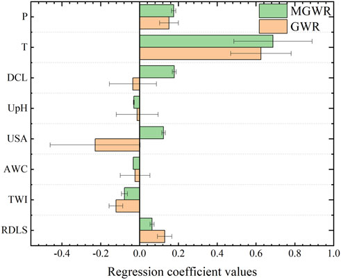
Figure 9. Comparison of regression coefficients for explanatory variables between the GWR and MGWR models. The bar shows the regression coefficients, and the whisker denotes the standard deviation of the coefficient estimations.
To understand the differences in environmental controls on the EHI among different functional types, the results of GWR models were further stratified by PFTs. T remains the most prominent control, regardless of the vegetation type. The LRC values of the variable T differed between the PFTs, with mean values of 0.67 ± 0.16 and 0.66 ± 0.21 for C3 and BDST, respectively, which were significantly higher (p < 0.05) than those of NETT, BDTT, and BDTB (Figure 10). The climatic variable P also exerted considerable influence on the EHI. There was no significant difference in the controls of P among the three arboreal vegetation types, with the LRCs being 0.19 ± 0.04, 0.20 ± 0.00, and 0.20 ± 0.02 for NETT, BDTT, and BDTB, respectively, while for BDST and C3, they are 0.17 ± 0.04 and 0.11 ± 0.05, respectively, suggesting less dependence on P compared to arboreal vegetation types. The control USA on the EHI appeared more discernable for BDST and C3, with mean LRC values of −0.16 ± 0.16 for BDST and −0.29 ± 0.15 for C3. The controls DCL and UpH on the EHI were insignificantly different among various PFTs. Unfavorable effects of TWI or AWC on EHI were found for all the PFTs, and non-significant differences were found in LRC values among the PFTs, either for TWI or for AWC.
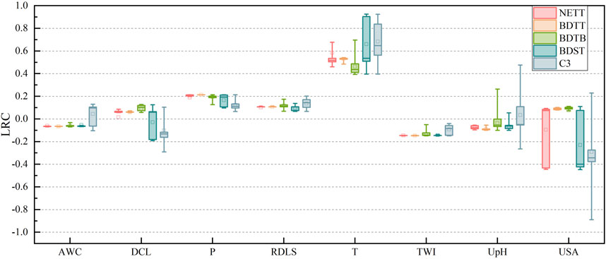
Figure 10. Stratified LRC values of the explanatory variables using the five PFTs. The box represents the IQR of LRC; the whiskers refer to the range within the first and third quartiles; the line inside the box represents the median; the hollow square indicates the mean value of the data; and the solid dots refer to outliers, which are anomalies that are significantly distant from the remaining data points. Different colors represent the LRC of explanatory variables for different PFTs.
4 Discussion
4.1 Environmental controls on the EHI of the region
Understanding the environmental controls on ecosystem health is a prerequisite for effective ecosystem restoration in the area (Rodriguez-Flores et al., 2025). We have used the OLS, GWR, and MGWR techniques to explore the potential environmental controls on the EHI in our natural watershed ecosystem.
Our study watershed is located in a transitional zone between the semi-arid and semi-humid regions of northern China. Although water stress is often considered a primary constraint on ecosystems of northern China (Xie et al., 2020; Huang et al., 2021; Zhang et al., 2022), our modeling analysis suggests that thermal stress is a major constraint on the development of ecosystem health in the Xiaoluan River watershed, irrespective of the PFTs, with a spatially average LRC value of 0.63 ± 0.15 across the area, which is considerably higher than that of other environmental variables. This result aligns with the findings of Guo et al. (2023), who found that temperature had a stronger influence on the spatial variation of vegetation productivity in similar areas than precipitation. The thermal stress of EHI herein can be easily understood because the vegetation growth and/or productivity in mountainous areas or humid bio-climates usually relies more heavily on available thermal resources (Karnieli et al., 2010; Bento et al., 2018; Veena et al., 2023). Moreover, our watershed is characterized by a mountainous terrain with elevations ranging from 769 m to 1,902 m, and it experiences a prolonged winter season, usually from October to mid-April, with a mean annual temperature of only 3.54 °C ± 1.77 °C.
We highlighted the primary key constraint of thermal stress on the EHI of the areas, but it does not follow that precipitation is irrelevant to the ecosystem of the watershed. This is especially true for tree plantations as the LRC values of P for arboreal vegetation were consistently higher than those for shrubs and C3 (Figure 9). Water stress was usually a major constraint for vegetation growth and/or productivity in arid and semi-arid areas (Miranda et al., 2011; Wu et al., 2020; Bai et al., 2023). Our watershed had limited water availability, with the mean annual precipitation being 414.6 ± 15.3 mm. This explains why the variable P, alongside T, had a considerable effect on the ecosystem in the area. However, due to the frequent occurrence of snowpack (Li et al., 2020), snowmelt water partially alleviated the constraining effects of precipitation on ecosystem health (Zhou et al., 2025), leading to the LRC values of P being relatively lower than those of T.
Although both T and P are the most pronounced controls on the EHI of the areas, we suggest that the two variables alternatively dominate the areas by season. By further examining seasonal models of the EHI, we found that the controls P and T differed by season (Figure 11). In other words, ecosystem health during the growing season was mainly controlled by P, while at the beginning of the growing season, the control shifted to T, which is critically important for leaf unfolding and sap flow, especially for the arboreal vegetation, potentially determining vegetation productivity for the year.
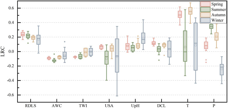
Figure 11. Seasonal distribution of LRC values of explanatory variables. The box represents the IQR of LRC; the whiskers refer to the range within the first and third quartiles; the line inside the box represents the median; the hollow square indicates the mean value of the data; the solid dots refer to outliers, which are anomalies that are significantly distant from the remaining data points. LRC values of explanatory variables representing different seasons with different colors.
One may note that both variables, TWI and AWC, which are widely considered proxies for soil moisture conditions (Raduła et al., 2018; Ladányi et al., 2021), exhibited negative effects on ecosystem health in the area. As mentioned previously, the high percentage of clay in the soil may partially explain the negative effects of the two variables on ecosystem health. Additionally, both Larix gmelinii and Pinus sylvestris are key species for revegetation, and both preferentially thrive in well-drained soil properties (Li D. et al., 2023); therefore, it is reasonable to believe that they exert a negative influence on the EHI of the area.
Regarding the soil variables, USA, UpH, and DCL, we found that they generally had minor effects on mediating ecosystem health in the area. This is particularly true for the PFTs NETT, BDTT, and BDTB (see Figure 9), where the LRC values are almost 0, suggesting minimal constraints imposed by sandy soil texture on vegetation health for tree species, which is in agreement with the findings of Cheng et al. (2023).
4.2 Implications for the resilience of ecosystem health
Ecosystem resilience has recently received increasing attention from researchers (Holling, 1973; Oliver et al., 2015; Anderegg et al., 2018; Wu et al., 2024). Various methods and/or frameworks were employed for resilience analysis. In the analysis performed by Wu et al. (2024), the authors utilized the NDVI as a proxy to estimate ecological resilience by combining a vegetation sensitivity index with the adaptability index and found that the resilience of their investigated area had improved overall from 2000 to 2020, but there were significant regional differences. Oliver et al. (2015) investigated how ecosystem resilience responds to biodiversity and the underlying mechanisms using redundancy analysis and path analysis based on controlled field experiments. Anderegg et al. (2018) analyzed ecosystem resilience at the stand scale and found that diversity in the hydraulic traits of the trees mediates ecosystem resilience to drought.
In our case, although we did not carry out a thorough analysis of resilience as in the above studies, the low ER value in the EHI—only 0.19—well-illustrated the relatively low level of ecosystem resilience in the area, likely due to the high temperature variability in the region. Moreover, Moran’s I of the EHI in the watershed was as high as 0.92 ± 0.01, showing a strong spatially positive autocorrelation. According to Sankaran et al. (2019), systems with strong positive spatial correlation are usually more prone to undergo abrupt transitions and exhibit lower resistance to system perturbations. Therefore, the high Moran’s I of the Xiaoluan River watershed actually indicates a lower level of resilience of the ecosystem health. This is in agreement with the results of the ER component in EHI analysis.
Both T and P were two primary controls on the ecosystem health of the watershed. Considering that climate change may be more intensified in future, with the increasing variability in temperature and precipitation (Hansen et al., 2013; He and Li, 2018; Cai et al., 2022), it should not be overlooked in relation to the ecosystem resilience of the watershed. As mentioned previously in the local Moran’s I section, both NETT and BDTT in the area were typically derived from man-made plantations and exhibited very strong positive spatial correlations within the watershed; the HH clustering areas accounted for as much as 75.05% and 97.33%, respectively, indicating a proneness to abrupt transitions in the event of environmental anomalies. We, therefore, suggest that more caution should be exercised with these PFTs when implementing revegetation activities to avoid possible ecosystem collapse and protect the ecosystem health of the natural watershed.
5 Conclusion
Assessing ecosystem health and understanding its environmental controls are valuable for effectively restoring natural ecosystems in mountainous areas and enhancing their resilience to environmental perturbations. We assessed the ecosystem health of a natural watershed (Xiaoluan River watershed) in the mountainous areas of northern China using the traditional VOR framework combined with Moran’s I analysis and explored environmental controls on ecosystem health using OLS, GWR, and MGWR modeling techniques.
We found that the ecosystem health of the Xiaoluan River watershed showed a slightly increasing trend from 2006 to 2020 as revegetation progressed, with the EHI varying from 0.49 to 0.57. However, the resilience of the ecosystem health of the watershed remained relatively low as the mean value of ER over the years was only 0.19. A strong positive spatial autocorrelation was identified using global Moran’s I, especially for the vegetation types NETT and BDTT, suggesting a proneness to abrupt transitions in the event of environmental perturbations. Both thermal stress and water stress were found to be dominant constraints on the variation in ecosystem health in the areas, with temperature mainly dominating at the beginning of the growing season and alternating with precipitation, which is dominant during the growing season. Regarding the pedological variables such as soil texture and other soil wetness variables, they had relatively less effect on vegetation health, especially for arboreal vegetation.
We concluded that, for the mountainous areas that are mainly revegetated with man-made plantations in northern China, the ecosystem health might not have increased as profoundly as anticipated since the ecosystem resilience of the areas remained at a relatively lower level, particularly in the planted forests. In the future, in the face of global climate change, greater caution should be exercised with man-made plantations when implementing revegetation policies in the area in order to avoid possible ecosystem collapse and enhance ecosystem resilience more effectively.
Data availability statement
The original contributions presented in the study are included in the article/Supplementary Material; further inquiries can be directed to the corresponding author.
Author contributions
SQ: Writing – original draft. SW: Writing – review and editing, Writing – original draft. FZ: Writing – review and editing. WL: Writing – review and editing. DC: Writing – review and editing. ZZ: Writing – review and editing. PS: Writing – review and editing. KW: Writing – review and editing. YL: Writing – review and editing.
Funding
The author(s) declare that financial support was received for the research and/or publication of this article. This study was financially supported by the National Key Research and Development Program of China (Grant No. 2022YFF1302501-02).
Acknowledgments
The authors would like to thank both the editors and the reviewers for their valuable suggestions and comments. The 1-km monthly mean precipitation and temperature datasets for china datasets were provided by the National Tibetan Plateau/Third Pole Environment Data Center (http://data.tpdc.ac.cn). The plant functional type map of China dataset was provided by the National Cryosphere Desert Data Center. (http://www.ncdc.ac.cn).
Conflict of interest
The authors declare that the research was conducted in the absence of any commercial or financial relationships that could be construed as a potential conflict of interest.
Generative AI statement
The author(s) declare that no Generative AI was used in the creation of this manuscript.
Publisher’s note
All claims expressed in this article are solely those of the authors and do not necessarily represent those of their affiliated organizations, or those of the publisher, the editors and the reviewers. Any product that may be evaluated in this article, or claim that may be made by its manufacturer, is not guaranteed or endorsed by the publisher.
References
Abbas, Z., Zhu, Z., and Zhao, Y. (2022). Spatiotemporal analysis of landscape pattern and structure in the greater Bay area, China. Earth Sci. Inf. 15 (3), 1977–1992. doi:10.1007/s12145-022-00782-y
Anderegg, W. R. L., Konings, A. G., Trugman, A. T., Yu, K., Bowling, D. R., Gabbitas, R., et al. (2018). Hydraulic diversity of forests regulates ecosystem resilience during drought. Nature 561 (7724), 538–541. doi:10.1038/s41586-018-0539-7
Bai, X., Fan, Z., and Yue, T. (2023). Dynamic pattern-effect relationships between precipitation and vegetation in the semi-arid and semi-humid area of China. Catena 232, 107425. doi:10.1016/j.catena.2023.107425
Bandak, S., Movahedi-Naeini, S. A., Mehri, S., and Lotfata, A. (2024). A longitudinal analysis of soil salinity changes using remotely sensed imageries. Sci. Rep. 14 (1), 10383. doi:10.1038/s41598-024-60033-6
Bao, Z., Shifaw, E., Deng, C., Sha, J., Li, X., Hanchiso, T., et al. (2022). Remote sensing-based assessment of ecosystem health by optimizing vigor-organization-resilience model: a case study in fuzhou city, China. Ecol. Inf. 72, 101889. doi:10.1016/j.ecoinf.2022.101889
Bento, V. A., Gouveia, C. M., DaCamara, C. C., and Trigo, I. F. (2018). A climatological assessment of drought impact on vegetation health index. Agric. For. Meteorology 259, 286–295. doi:10.1016/j.agrformet.2018.05.014
Bertoldi, G., Chiesa, D. S., Notarnicola, C., Pasolli, L., Niedrist, G., and Tappeiner, U. (2014). Estimation of soil moisture patterns in mountain grasslands by means of SAR RADARSAT2 images and hydrological modeling. J. Hydrol. 516, 245–257.
Brunsdon, C., Fotheringham, A. S., and Charlton, M. E. (2010). Geographically weighted regression: a method for exploring spatial nonstationarity. Geogr. Anal. 28 (4), 281–298. doi:10.1111/j.1538-4632.1996.tb00936.x
Buchanan, B. P., Fleming, M., Schneider, R. L., Richards, B. K., Archibald, J., Qiu, Z., et al. (2014). Evaluating topographic wetness indices across central New York agricultural landscapes. Hydrology Earth Syst. Sci. 18 (8), 3279–3299. doi:10.5194/hess-18-3279-2014
Cai, W., Ng, B., Wang, G., Santoso, A., Wu, L., and Yang, K. (2022). Increased ENSO sea surface temperature variability under four IPCC emission scenarios. Nat. Clim. Change 12 (3), 228–231. doi:10.1038/s41558-022-01282-z
Cartwright, J. M., Littlefield, C. E., Michalak, J. L., Lawler, J. J., and Dobrowski, S. Z. (2020). Topographic, soil, and climate drivers of drought sensitivity in forests and shrublands of the Pacific northwest, USA. Sci. Rep. 10 (1), 18486. doi:10.1038/s41598-020-75273-5
Cheng, R., Zhang, J., Wang, X., Ge, Z., and Zhang, Z. (2023). Predicting the growth suitability of larix principis-rupprechtii mayr based on site index under different climatic scenarios. Front. Plant Sci. 14, 1097688. doi:10.3389/fpls.2023.1097688
Chu, X., Zhan, J., Li, Z., Zhang, F., and Qi, W. (2019). Assessment on forest carbon sequestration in the three-north shelterbelt program region, China. J. Clean. Prod. 215, 382–389. doi:10.1016/j.jclepro.2018.12.296
Costanza, R., D'Arge, R., De Groot, R., Farber, S., Grasso, M., Hannon, B., et al. (1997). The value of the world's ecosystem services and natural capital. Nature 387 (6630), 253–260. doi:10.1038/387253a0
Cunha, A. P. M., Alvalá, R. C., Nobre, C. A., and Carvalho, M. A. (2015). Monitoring vegetative drought dynamics in the Brazilian semiarid region. Agric. For. Meteorology 214-215, 494–505. doi:10.1016/j.agrformet.2015.09.010
Duan, H., Yan, C., Tsunekawa, A., Song, X., Li, S., and Xie, J. (2011). Assessing vegetation dynamics in the three-north shelter forest region of China using AVHRR NDVI data. Environ. Earth Sci. 64 (4), 1011–1020. doi:10.1007/s12665-011-0919-x
Fotheringham, A. S., Yang, W., and Kang, W. (2017). Multiscale geographically weighted regression (MGWR). Ann. Am. Assoc. Geogr. 107 (6), 1247–1265. doi:10.1080/24694452.2017.1352480
Fu, W. J., Jiang, P. K., Zhou, G. M., and Zhao, K. L. (2014). Using Moran's I and GIS to study the spatial pattern of forest litter carbon density in a subtropical region of southeastern China. Biogeosciences 11 (8), 2401–2409. doi:10.5194/bg-11-2401-2014
Gao, Y., Zhao, J., and Yu, K. (2022). Effects of block morphology on the surface thermal environment and the corresponding planning strategy using the geographically weighted regression model. Build. Environ. 216, 109037. doi:10.1016/j.buildenv.2022.109037
Ge, F., Tang, G., Zhong, M., Zhang, Y., Xiao, J., Li, J., et al. (2022). Assessment of ecosystem health and its key determinants in the middle reaches of the yangtze river urban agglomeration, China. Int. J. Environ. Res. Public Health 19 (2), 771. doi:10.3390/ijerph19020771
Guo, H., Yuan, J.-g., Wang, J.-z., Wang, X.-x., Li, Y.-c., and Liu, B.-h. (2023). Spatio-temporal evolution of net primary productivity in beijing-tianjin-hebei region based on MOD17A3 data. J. Changjiang River Sci. Res. Inst. 40. doi:10.11988/ckyyb.20220164
Hansen, J., Sato, M., Russell, G., and Kharecha, P. (2013). Climate sensitivity, sea level and atmospheric carbon dioxide. Philosophical Trans. R. Soc. A Math. Phys. Eng. Sci. 371 (2001), 20120294. doi:10.1098/rsta.2012.0294
Harries, K. (2006). Extreme spatial variations in crime density in Baltimore county, MD. Geoforum 37 (3), 404–416. doi:10.1016/j.geoforum.2005.09.004
He, C., and Li, T. (2018). Does global warming amplify interannual climate variability? Clim. Dyn. 52 (5-6), 2667–2684. doi:10.1007/s00382-018-4286-0
He, J., Pan, Z., Liu, D., and Guo, X. (2019). Exploring the regional differences of ecosystem health and its driving factors in China. Sci. Total Environ. 673, 553–564. doi:10.1016/j.scitotenv.2019.03.465
Holling, C. S. (1973). “Resilience and stability of ecological systems,” in Foundations of socio-environmental research: legacy readings with commentaries. Editors W. R. Burnside, S. Pulver, K. J. Fiorella, M. L. Avolio, and S. M. Alexander (Cambridge: Cambridge University Press), 460–482.
Houyun, S., Xiaofeng, W., Xiaoming, S., Fengchao, J., Duojie, L., Zexin, H., et al. (2020). Formation mechanism and geological construction constraints of metasilicate mineral water in yudaokou hannuoba basalt area. Earth Sci. 45 (11), 4236–4253. doi:10.3799/dqkx.2020.011
Huang, C., Liang, Y., He, H. S., Wu, M. M., Liu, B., and Ma, T. (2021). Sensitivity of aboveground biomass and species composition to climate change in boreal forests of northeastern China. Ecol. Model. 445, 109472. doi:10.1016/j.ecolmodel.2021.109472
Huang, J., Liu, X., Liu, J., Zhang, Z., Zhang, W., Qi, Y., et al. (2023). Changes of soil bacterial community, network structure, and carbon, nitrogen and sulfur functional genes under different land use types. Catena 231, 107385. doi:10.1016/j.catena.2023.107385
Ibrahim, Y., Balzter, H., Kaduk, J., and Tucker, C. (2015). Land degradation assessment using residual trend analysis of GIMMS NDVI3g, soil moisture and rainfall in sub-saharan West Africa from 1982 to 2012. Remote Sens. 7 (5), 5471–5494. doi:10.3390/rs70505471
Jiang, R., Liang, J., Zhao, Y., Wang, H., Xie, J., Lu, X., et al. (2021). Assessment of vegetation growth and drought conditions using satellite-based vegetation health indices in jing-jin-ji region of China. Sci. Rep. 11 (1), 13775. doi:10.1038/s41598-021-93328-z
Kalwa, V., Ullegaddi, M. M., Kittali, P., and Thottempudi, B. (2023). Ordinary least square regression technique for predicting wear rate of EN8 carbon steel. Mater. Today Proc. doi:10.1016/j.matpr.2023.03.388
Karnieli, A., Agam, N., Pinker, R. T., Anderson, M., Imhoff, M. L., Gutman, G. G., et al. (2010). Use of NDVI and land surface temperature for drought assessment: merits and limitations. J. Clim. 23 (3), 618–633. doi:10.1175/2009JCLI2900.1
Khalid, W., Kausar Shamim, S., and Ahmad, A. (2024). Exploring urban land surface temperature with geospatial and regression modelling techniques in Uttarakhand using SVM, OLS and GWR models. Evol. Earth 2, 100038. doi:10.1016/j.eve.2024.100038
Kopecký, M., Macek, M., and Wild, J. (2021). Topographic wetness index calculation guidelines based on measured soil moisture and plant species composition. Sci. Total Environ. 757, 143785. doi:10.1016/j.scitotenv.2020.143785
Ladányi, Z., Barta, K., Blanka, V., and Pálffy, B. (2021). Assessing available water content of sandy soils to support drought monitoring and agricultural water management. Water Resour. Manag. 35 (3), 869–880. doi:10.1007/s11269-020-02747-6
Li, M. M., Liu, A. T., Zou, C. J., Xu, W. D., Shimizu, H., and Wang, K.-y. (2012). An overview of the “Three-North” shelterbelt project in China. For. Stud. China 14 (1), 70–79. doi:10.1007/s11632-012-0108-3
Li, X., Liang, S., Zhao, K., Wang, J., Che, T., and Li, Z. (2020). Snow cover classification based on climate variables and its distribution characteristics in China. J. Glaciol. Geocryol. 42 (1), 62–71. doi:10.7522/j.issn.1000-0240.2019.0050
Li, D., Li, J., Gao, G., Zhang, Y., Ren, Y., Liu, Y., et al. (2023a). Soil fungal community structure and functional characteristics associated with pinussylvestris Var. mongolica plantations in the horqin sandy land. J. Desert Res. 43 (4), 241–251. doi:10.7522/j.issn.1000-694X.2023.00035
Li, M., Luo, G., Li, Y., Qin, Y., Huang, J., and Liao, J. (2023b). Effects of landscape patterns and their changes on ecosystem health under different topographic gradients: a case study of the miaoling Mountains in southern China. Ecol. Indic. 154, 110796. doi:10.1016/j.ecolind.2023.110796
Li, K. M., Wang, X.-Y., and Yao, L.-L. (2024a). Spatial-temporal evolution of ecosystem health and its influencing factors in beijing-tianjin-hebei region. Huan jing ke xue= Huanjing kexue 45 (1), 218–227. doi:10.13227/j.hjkx.202301077
Li, M., Abuduwaili, J., Liu, W., Feng, S., Saparov, G., and Ma, L. (2024b). Application of geographical detector and geographically weighted regression for assessing landscape ecological risk in the irtysh river basin, central Asia. Ecol. Indic. 158, 111540. doi:10.1016/j.ecolind.2023.111540
Liu, M., and Dong, G.-h. (2006). RS and GIS support of the ecological environment health evaluation in qinhuangdao area. Geogr. Res. 25 (5), 930–938. doi:10.11821/yj2006050019
Liu, X., Li, P., Ren, Z., Miao, Z., Zhang, J., Liu, X., et al. (2016). Evaluation of ecosystem resilience in yulin, China. Acta Ecol. Sin. 26, 7479–7491. doi:10.5846/stxb201601120071
López, D. R., Brizuela, M. A., Willems, P., Aguiar, M. R., Siffredi, G., and Bran, D. (2013). Linking ecosystem resistance, resilience, and stability in steppes of north patagonia. Ecol. Indic. 24, 1–11. doi:10.1016/j.ecolind.2012.05.014
Ma, J., Ding, X., Shu, Y., and Abbas, Z. (2022). Spatio-temporal variations of ecosystem health in the liuxi river basin, guangzhou, China. Ecol. Inf. 72, 101842. doi:10.1016/j.ecoinf.2022.101842
Martínez, B., and Gilabert, M. A. (2009). Vegetation dynamics from NDVI time series analysis using the wavelet transform. Remote Sens. Environ. 113 (9), 1823–1842. doi:10.1016/j.rse.2009.04.016
Meng, X., and Wang, H. (2018). Siol map based harmonized world soil database (v1. 2). Beijing, China: National Tibetan Plateau Data Center.
Miranda, J. D., Armas, C., Padilla, F. M., and Pugnaire, F. I. (2011). Climatic change and rainfall patterns: effects on semi-arid plant communities of the iberian southeast. J. Arid Environ. 75 (12), 1302–1309. doi:10.1016/j.jaridenv.2011.04.022
Na, L., Shi, Y., and Guo, L. (2023). Quantifying the spatial nonstationary response of influencing factors on ecosystem health based on the geographical weighted regression (GWR) model: an example in Inner Mongolia, China, from 1995 to 2020. Environ. Sci. Pollut. Res. 30 (29), 73469–73484. doi:10.1007/s11356-023-26915-4
Oliver, T. H., Heard, M. S., Isaac, N. J. B., Roy, D. B., Procter, D., Eigenbrod, F., et al. (2015). Biodiversity and resilience of ecosystem functions. Trends Ecol. and Evol. 30 (11), 673–684. doi:10.1016/j.tree.2015.08.009
Ouyang, N., Rui, X., Zhang, X., Tang, H., and Xie, Y. (2024). Spatiotemporal evolution of ecosystem health and its driving factors in the Southwestern karst regions of China. Ecol. Indic. 166, 112530. doi:10.1016/j.ecolind.2024.112530
Pan, Z., He, J., Liu, D., Wang, J., and Guo, X. (2021). Ecosystem health assessment based on ecological integrity and ecosystem services demand in the middle reaches of the yangtze river economic belt, China. Sci. Total Environ. 774, 144837. doi:10.1016/j.scitotenv.2020.144837
Peng, S. (2024a). Data from: 1-Km monthly mean temperature dataset for China (1901-2023). Beijing: National Tibetan Plateau Data Center. doi:10.11888/Meteoro.tpdc.270961
Peng, S. (2024b). Data from: 1-Km monthly precipitation dataset for China (1901-2023). Beijing: National Tibetan Plateau Data Center. doi:10.5281/zenodo.3114194
Peng, J., Liu, Y., Li, T., and Wu, J. (2017). Regional ecosystem health response to rural land use change: a case study in lijiang city, China. Ecol. Indic. 72, 399–410. doi:10.1016/j.ecolind.2016.08.024
Raduła, M. W., Szymura, T. H., and Szymura, M. (2018). Topographic wetness index explains soil moisture better than bioindication with Ellenberg’s indicator values. Ecol. Indic. 85, 172–179. doi:10.1016/j.ecolind.2017.10.011
Ran, Y. (2019). Data from: plant functional types map of China. Available online at: http://www.ncdc.ac.cn/portal/metadata/aa4460d1-b99a-4531-bd44-0d6509326762.
Rodriguez-Flores, S., Muñoz-Robles, C., Quevedo Tiznado, J. A., and Julio-Miranda, P. (2025). Assessment of watershed health, integrating environmental, social, and climate change criteria into a fuzzy logic framework. Sci. Total Environ. 960, 178316. doi:10.1016/j.scitotenv.2024.178316
Sankaran, S., Majumder, S., Viswanathan, A., Guttal, V., and Ye, H. (2019). Clustering and correlations: inferring resilience from spatial patterns in ecosystems. Methods Ecol. Evol. 10 (12), 2079–2089. doi:10.1111/2041-210x.13304
Shao, Y., Liu, Y., Ma, T., Sun, L., Yang, X., Li, X., et al. (2023). Conservation effectiveness assessment of the three northern protection forest project area. Forests 14 (11), 2121. doi:10.3390/f14112121
Shen, W., Zheng, Z., Qin, Y., and Li, Y. (2020). Spatiotemporal characteristics and driving force of ecosystem health in an important ecological function region in China. Int. J. Environ. Res. Public Health 17 (14), 5075. doi:10.3390/ijerph17145075
Shen, W., Zheng, Z., Pan, L., Qin, Y., and Li, Y. (2021). A integrated method for assessing the urban ecosystem health of rapid urbanized area in China based on SFPHD framework. Ecol. Indic. 121, 107071. doi:10.1016/j.ecolind.2020.107071
Shi, C., Miao, X., Zhang, L., Chiu, Y.-H., Zeng, Q., and Zhang, C. (2022). Spatial patterns of industrial water efficiency and influencing factors —Based on dynamic two-stage DDF recycling model and geographically weighted regression model. J. Clean. Prod. 374, 134028. doi:10.1016/j.jclepro.2022.134028
Song, S., Wang, S., Gong, Y., and Yu, Y. (2024). The past and future dynamics of ecological resilience and its spatial response analysis to natural and anthropogenic factors in southwest China with typical karst. Sci. Rep. 14 (1), 19166. doi:10.1038/s41598-024-70139-6
Teng, H., Chen, S., Hu, B., and Shi, Z. (2023). Future changes and driving factors of global peak vegetation growth based on CMIP6 simulations. Ecol. Inf. 75, 102031. doi:10.1016/j.ecoinf.2023.102031
Thakur, S., Negi, V. S., Dhyani, R., Satish, K. V., and Bhatt, I. D. (2021). Vulnerability assessments of Mountain forest ecosystems: a global synthesis. Trees, For. People 6, 100156. doi:10.1016/j.tfp.2021.100156
Veena, D., Amanpreet, K., Mehak, S., and Gosangi, A. (2023). “Perspective chapter: effect of low-temperature stress on plant performance and adaptation to temperature change,” in Plant abiotic stress responses and tolerance mechanisms. Editors H. Saddam, A. Tahir Hussain, W. Ejaz Ahmad, and A. M. Iqbal (Rijeka: IntechOpen). Ch. 5.
Wang, C., Fu, B., Zhang, L., and Xu, Z. (2018). Soil moisture–plant interactions: an ecohydrological review. J. Soils Sediments 19 (1), 1–9. doi:10.1007/s11368-018-2167-0
Wang, J., Hu, A., Meng, F., Zhao, W., Yang, Y., Soininen, J., et al. (2022). Embracing Mountain microbiome and ecosystem functions under global change. New Phytol. 234 (6), 1987–2002. doi:10.1111/nph.18051
Won, J., and Kim, S. (2023). Ecological drought condition index to monitor vegetation response to meteorological drought in Korean peninsula. Remote Sens. 15 (2), 337. doi:10.3390/rs15020337
Wu, Y., Zhang, X., Fu, Y., Hao, F., and Yin, G. (2020). Response of vegetation to changes in temperature and precipitation at a semi-arid area of northern China based on multi-statistical methods. Forests 11 (3), 340. doi:10.3390/f11030340
Wu, J., Yang, M., Zuo, J., Yin, N., Yang, Y., Xie, W., et al. (2024). Spatio-temporal evolution of ecological resilience in ecologically fragile areas and its influencing factors: a case study of the wuling Mountains area, China. Sustainability 16 (9), 3671. doi:10.3390/su16093671
Xie, S., Mo, X., Hu, S., and Chen, X. (2020). Response of vegetation greenness to temperature and precipitation in the three-north shelterbelt program project area. Geogr. Res. 39 (1), 152–165. doi:10.11821/dlyj020181071
Xu, B., and Lin, B. (2017). Factors affecting CO 2 emissions in China’s agriculture sector: evidence from geographically weighted regression model. Energy Policy 104, 404–414. doi:10.1016/j.enpol.2017.02.011
Yang, J., and Huang, X. (2021). 30 m annual land cover and its dynamics in China from 1990 to 2019. Earth Syst. Sci. Data Discuss. 2021, 1–29. doi:10.5194/essd-13-3907-2021
Yin, P., Li, C., Wei, Y., Zhang, L., Liu, C., Chen, J., et al. (2024). Impact of relative temperature changes on vegetation growth in China from 2001 to 2017. J. Clean. Prod. 451, 142062. doi:10.1016/j.jclepro.2024.142062
Yu, H., and Peng, Z.-R. (2019). Exploring the spatial variation of ridesourcing demand and its relationship to built environment and socioeconomic factors with the geographically weighted poisson regression. J. Transp. Geogr. 75, 147–163. doi:10.1016/j.jtrangeo.2019.01.004
Yushanjiang, A., Zhang, F., and Tan, M. L. (2021). Spatial-temporal characteristics of ecosystem health in central Asia. Int. J. Appl. Earth Observation Geoinformation 105, 102635. doi:10.1016/j.jag.2021.102635
Zhai, J., Wang, L., Liu, Y., Wang, C., and Mao, X. (2023). Assessing the effects of China's three-north shelter forest program over 40 years. Sci. Total Environ. 857, 159354. doi:10.1016/j.scitotenv.2022.159354
Zhang, J., and Zhang, Y. (2024). Quantitative assessment of the impact of the three-north shelter forest program on vegetation net primary productivity over the past two decades and its environmental benefits in China. Sustainability 16 (9), 3656. doi:10.3390/su16093656
Zhang, C., Luo, L., Xu, W., and Ledwith, V. (2008). Use of local Moran's I and GIS to identify pollution hotspots of Pb in urban soils of Galway, Ireland. Sci. Total Environ. 398 (1-3), 212–221. doi:10.1016/j.scitotenv.2008.03.011
Zhang, X., Xu, Y., Hao, F., and Hao, Z. (2022). Characteristics and risk analysis of droughtpropagation from meteorological droughtto hydrological drought in luanhe river basin. J. Hydrology Eng. 53, 165–175. doi:10.13243/j.cnki.slxb.20210477
Zhou, Y., Yue, D., Li, S., Liang, G., Chao, Z., Zhao, Y., et al. (2022). Ecosystem health assessment in debris flow-prone areas: a case study of bailong river basin in China. J. Clean. Prod. 357, 131887. doi:10.1016/j.jclepro.2022.131887
Zhou, F., Wang, S., Qu, S., Li, W., Cai, D., Hai, Q., et al. (2025). Understanding hydrological process change due to re-vegetation in a mountainous watershed of northern China. Hydrol. Process. 39 (3). doi:10.1002/hyp.70103
Keywords: ecosystem health assessment, environmental controls, vigor–organization–resilience framework, geographically weighted regression modeling, mountainous watershed
Citation: Qu S, Wang S, Zhou F, Li W, Cai D, Zhang Z, Strauss P, Wang K and Liu Y (2025) Assessing ecosystem health following revegetation in the mountainous areas of northern China. Front. Earth Sci. 13:1614748. doi: 10.3389/feart.2025.1614748
Received: 19 April 2025; Accepted: 22 July 2025;
Published: 22 August 2025.
Edited by:
Eduardo Gomes, University of Lisbon, PortugalReviewed by:
Ying Zhu, Xi’an University of Architecture and Technology, ChinaZhihua Zhang, Shandong University, China
Copyright © 2025 Qu, Wang, Zhou, Li, Cai, Zhang, Strauss, Wang and Liu. This is an open-access article distributed under the terms of the Creative Commons Attribution License (CC BY). The use, distribution or reproduction in other forums is permitted, provided the original author(s) and the copyright owner(s) are credited and that the original publication in this journal is cited, in accordance with accepted academic practice. No use, distribution or reproduction is permitted which does not comply with these terms.
*Correspondence: Shengping Wang, c2hlbmdwaW5nX3dhbmdAbmNlcHUuZWR1LmNu, bmNlcHVfcXVzaXlpQDE2My5jb20=