Utilizing dense magnetotelluric array to analyze deep seismogenic environment in the Huaibei plain fold belt

The Huaibei Plain Fold Belt, located on the southeastern margin of the North China Plate, lies adjacent to the Tancheng-Lujiang fault zone—one of the most active fault zones in eastern China—characterized by complex tectonic activity. Using a 3D dense magnetotelluric (MT) array, we obtained high-quality MT data through fine time-series processing technology. Dimensionality and structural characteristics were analyzed using phase tensor analysis and statistical imaging of the impedance tensor. A fine and reliable 3D resistivity structure was constructed through nonlinear inversion, combining impedance data with a multiple iterative reconstruction technique. The results reveal that the high-resistivity and low-resistivity areas at shallow depths correspond to the Xuhuai arcuate tectonic structure and the Suzhou-Haogou Basin, respectively, with prominent low-resistivity anomalies present in the middle and lower crust. Beneath the Suzhou-Haogou Basin, blind low-resistivity faults are embedded within high-resistivity media and appear to be connected to deeper low-resistivity anomalies. These low-resistivity features are interpreted as the result of intense tectonic deformation and the presence of crustal fluids. There is no evidence of mantle-derived thermal upwelling, suggesting that deep mantle processes have limited influence on current tectonic deformation. Our findings indicate that the Huaibei Plain Fold Belt hosts a deep structural setting capable of generating strong earthquakes, with deformation primarily driven by horizontal tectonic forces. However, the underlying mechanism driving this deformation requires further investigation.

1 Introduction

Because earthquakes are among the natural disasters that cause the greatest casualties and economic losses, scientifically evaluating their likelihood has become a major priority in geoscientific research. Long-term studies have shown that earthquake generation is primarily influenced by the interplay between deep crustal structures and the regional geodynamic environment. Therefore, investigating the regional seismogenic environment is fundamental to assessing seismic hazard. The Huaibei Plain Fold Belt is located on the southeastern margin of the North China Plate, within the south-central segment of the Xuhuai arcuate tectonic belt, and lies adjacent to the Tancheng-Lujiang fault zone, one of the most active fault zones in eastern China. Historically, the region has experienced three destructive earthquakes, the largest been an M5¹/₂ earthquake in 1537, and minor earthquakes have been relatively frequent in recent years. Evaluating the deep seismogenic environment of the Huaibei Plain Fold Belt is therefore of great significance for assessing seismic hazard and supporting earthquake preparedness and mitigation efforts.

Numerous previous geophysical studies have investigated the broader study area. These include the large-scale P-wave velocity structures derived from teleseismic body waves (Lei et al., 2020; Tian et al., 2020; Sun et al., 2023); group velocity and phase velocity distributions based on ambient noise imaging (Gu et al., 2020; 2022; Ma et al., 2020); and a 3D isotropic S-wave velocity model inverted from continuous data collected by dense seismic arrays (Meng et al., 2019). However, most of these studies are conducted at regional or larger scales, and their spatial resolution is insufficient for detailed investigations of the seismogenic environment in specific zones of the study area. This highlights the need for high-resolution imaging of fine crustal structures. In recent years, with the advancement of 3D magnetotelluric (MT) inversion techniques, this method has been successfully applied to resolve fine-scale subsurface features in geologically complex regions (Cai et al., 2017; 2023; Rong et al., 2022; Xiao et al., 2022; Liu et al., 2024).

With the support of the Suzhou Active Fault Project and based on data from a dense magnetotelluric (MT) array, we constructed a high-resolution 3D electrical resistivity model of the Huaibei Plain Fold Belt. In addition, by integrating geological data with high-precision microearthquake relocation results, gravity anomalies, and regional stress field information, we conducted a comprehensive analysis of the deep seismogenic environment and explored potential earthquake-generating mechanisms.

The Huaibei Plain Fold Belt is situated on the southeastern margin of the North China Plate. It is bounded by the Tancheng–Lujiang Fault Zone (TLFZ) to the east, the Zhoukou Depression (ZKD) to the west, the Luxi Uplift to the north, and the Xubeng Uplift (XBU) to the south (Figure 1). This region is characterized by complex tectonic activity. The study area lies primarily within the Huaibei Plain Fold Belt, where the major structural trends are NE–NNE and EW. In addition, Cenozoic basins are relatively well developed. The large-scale Suzhou–Haogou Basin (SHB) formed during the Early Cretaceous under the influence of the Subei Fault (SBF) and the Guzhen–Huaiyuan Fault (GHF). Sediments from the Late Cretaceous and Paleocene are absent, and during the Eocene, the fluvial–lacustrine facies migrated southwestward, giving rise to an east–west–trending Cenozoic basin.

Figure 1

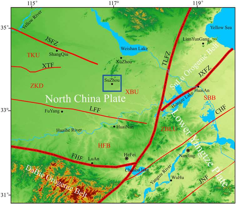
Figure 1. Schematic illustration of the tectonic background in the study area. TKU, Taikang Uplift; ZKD, Zhoukou Depression; XBU, Xubeng Uplift; HFB, Hefei Basin; SBB, Subei Basin; ZBLU, ZhangbaLing Uplift; TLFZ, Tancheng-Lujiang Fault Zone; FHF, Feixi-Hanbaidu Fault; JXFZ, Jiashan-Xiangshui Fault Zone; JSFZ, Jiaozuo-Shangqiu Fault Zone; XTF, Xuchang-Taikang Fault; LFF, Liufu Fault; CHF, Chuhe Fault; JNF, Jiangnan Fault. The blue box marks the position of the study area.

Tectonic activity in the study area is complex, with nearly ten large-scale faults identified (Figure 2). Overall, the region is characterized by weak tectonic activity. Most faults are dated to the Early to Middle Pleistocene, with a few originating prior to the Quaternary. The Subei Fault (SBF) is a blind fault that appears prominently in remote sensing imagery as a basin–range boundary-controlling structure. It marks the boundary between the arcuate tectonic mountains to the north and the Suzhou–Haogou Basin to the south. The Nanping Fault (NPF) is situated within zones of gravity and magnetic anomalies, intersecting a block with strong magnetic signatures. It defines the eastern boundary of the Cenozoic Nanping Basin. The Xisipo Fault (XSPF) is a thrust fault developed on the eastern limb of the Sunan syncline. It is associated with a series of similarly trending thrust faults and secondary folds, and may serve as a boundary fault of the arcuate tectonic system. Its most recent activity is dated to the Middle Pleistocene. The Guzhen–Huaiyuan Fault (GHF) appears in Bouguer gravity anomaly maps as a north–south–oriented gravity low zone superimposed on an east–west–oriented pattern of alternating positive and negative anomalies, suggesting strong structural control over regional tectonic landforms.

Figure 2

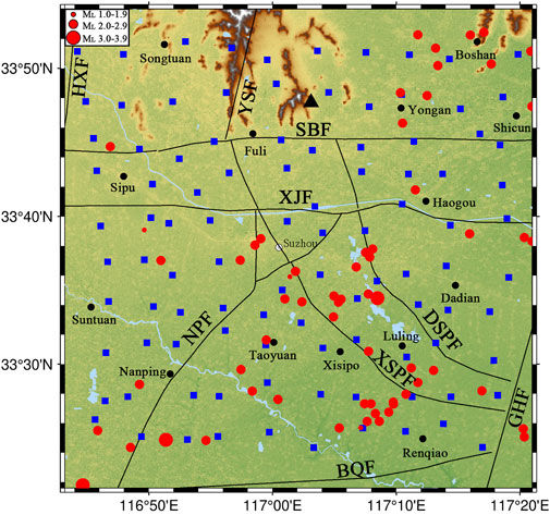
Figure 2. Locations of MT sites and relocated earthquakes. SBF, Subei Fault; XJF, Xinjia Fault; NPF, Nanping Fault; XSPF, Xisipo Fault; DSPF, Dongsanpu Fault; HXF, Huaibei-Xiaoxian Fault; YSF, Yingshan Fault; BQF, Banqiao Fault; GHF, Guzhen-Huaiyuan Fault. Earthquakes from 1976 to 2022 are marked as red circles scaled by magnitude. Blue squares mark the locations of MT sites and black triangles mark seismic stations.

Modern instrumental records indicate that the study area is characterized by low seismicity, predominantly featuring minor to moderate earthquakes. To better understand the spatial distribution of seismic activity, official seismic phase reports and earthquake catalogs from June 1976 to December 2024 were collected. These datasets include origin time, epicenter coordinates, focal depth, and P- and S-wave arrival times. Using the HYPO2000 absolute location algorithm and the CRUST2.0 velocity model, all recorded events were relocated (Figure 2). The relocation results show that earthquakes are mainly concentrated in the southern part of the study area, particularly along the Xisipo Fault (XSPF) and Dongsanpu Fault (DSPF), with their spatial distribution aligning with the fault trends. In contrast, seismic events in the northern region are more scattered and exhibit no obvious clustering. Overall, seismic activity in the region is weak, with relatively few small earthquakes.

2 Data and methods

A 3D dense magnetotelluric (MT) array survey was conducted across a 50 km × 50 km area in the Huaibei Plain Fold Belt (Figure 2). Field measurements employed a combination of large- and small-spacing deployments using the phase-interval array observation technique, which shortens observation time, enhances the reliability of inversion results, and maintains the resolution of shallow structures (Zhang et al., 2025). A total of 100 broadband MT sites were completed. Among them, 25 sites had a spacing of 10 km, with observation durations exceeding 35 h and valid data periods longer than 1000 s. The remaining 75 sites were spaced at 5 km, with observation times over 5 h and data validity periods exceeding 100 s.

Field data were acquired using the MTU-5A magnetotelluric system manufactured by Phoenix Geophysics (Canada). To improve data quality and suppress noise interference in the study area, the remote magnetic reference technique was employed (Gamble et al., 1979). A remote reference station was established in Liuzhou City, Guangxi—approximately 1,200 km from the survey area—at a site characterized by low electromagnetic noise and relatively simple geological conditions. The reference station recorded continuously and operated synchronously with field observations in the study area.

2.1 Time series processing

The study area is primarily located within urban zones, characterized by dense transportation infrastructure, including roads and railways. Residential settlements are widely distributed across the plain, and several MT sites were inevitably affected by anthropogenic interference, resulting in elevated electromagnetic noise levels that degraded data quality.

To mitigate this problem, researchers have introduced the remote reference observation technique in combination with robust time-series processing algorithms (Egbert and Booker, 1986). The core principle of the remote reference method is to deploy a continuously recording station 100–500 km away from the survey area, ideally in a region with minimal electromagnetic noise and simple geological conditions. During time-series processing, data segments that exhibit the highest correlation with the reference signal are extracted. Spectral analyses of these segments are then used to calculate the magnetotelluric (MT) response functions. In practice, this technique has proven highly effective in enhancing MT data quality by suppressing uncorrelated noise.

In contrast, the Robust processing algorithm is an adaptive method that selects time-window segments based on the correlation between the local station’s electric and magnetic field components. Segments with higher correlation are presumed to yield more reliable magnetotelluric (MT) responses. However, this assumption fails in the presence of stable, local alternating-field sources, which can artificially elevate E–B field correlation. As a result, poor-quality data may be retained while high-quality spectral segments are discarded. This issue is particularly prevalent in eastern China, where the dense power grid introduces widespread coherent electromagnetic interference. Under such conditions, correlation-based segment selection becomes ineffective, and the Robust processing algorithm may ultimately degrade rather than improve data quality.

Given the principles of remote reference and robust processing discussed above, it is evident that using a remote reference station as a correlation template is well justified—such stations are typically located in electromagnetically quiet areas with relatively simple geological settings. In contrast, the robust algorithm selects time-window segments based on the local correlation between electric and magnetic fields, which does not always guarantee the identification of high-quality spectra. Since the subsequent processing involves spectral selection and stacking, it is prudent to retain as much potentially useful data as possible when high-quality spectra cannot be reliably distinguished, rather than risk discarding valuable segments. Therefore, a larger number of stacking groups should be employed during data processing. For instance, the conventional approach typically divides the data into 20 groups, generating 20 stacked spectra for selection. In our workflow, we increase the number of groups to 40, or even 100. Although this results in a more complex and time-consuming selection process, it often eliminates the need for repeated or supplementary field surveys—conserving both time and resources and ultimately improving operational efficiency.

In this study, the Robust processing technique was used to suppress uncorrelated random noise during time-series data processing. To address strong near-field interference caused by highly correlated electromagnetic noise in source-proximal areas, we adopted a combined approach incorporating remote magnetic reference, non-Robust processing, and fine spectral editing techniques (Zhang et al., 2022). The results demonstrate that this method is particularly effective in mitigating mid-frequency near-field interference (Figure 3). In the original data, affected by interference, the mid-frequency phase approaches 0°, and the apparent resistivity curve increases by more than 45°—a typical signature of near-field contamination in urban environments. After applying the combined processing strategy, the interference is effectively removed, resulting in smoother and more continuous curves, and a significant improvement in data quality.

Figure 3

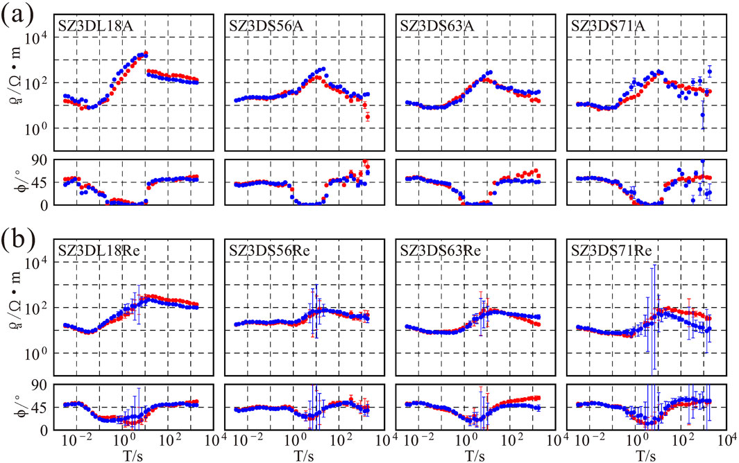
Figure 3. Comparison of the MT responses using different time-series processing methods. (a) Results without remote reference. (b) Results with remote reference and non-Robust estimation.

2.2 Qualitative analysis

After acquiring the observational data, qualitative analysis can reveal fundamental characteristics of the subsurface geological structure and provide valuable constraints for interpreting the inversion results. In this study, we utilized the MT-Pioneer (Chen et al., 2004)visual integration system for impedance tensor decomposition and dimensionality analysis.

The phase tensor provides a qualitative assessment of the macroscopic geometric characteristics of the regional electrical structure (Caldwell et al., 2004; Patro et al., 2013; Tietze et al., 2015). The two-dimensional skew angle (β) represents the deviation of the phase tensor from the principal axis of its equivalent symmetric tensor. Under ideal conditions, a β value greater than 0° suggests a three-dimensional (3D) electrical structure. However, due to observational noise and processing errors, a threshold of β > 5° is generally accepted as indicative of a 3D regional structure (Booker, 2014).

The geometric mean (φ₂) of the maximum and minimum phase differences between the magnetic and electric fields is used to represent the average phase variation along the polarization direction (Heise et al., 2008). The φ₂ parameter is not affected by local distortion or static shift. High φ₂ values suggest increasing conductivity with depth, whereas low φ₂ values indicate a trend toward higher resistivity. Although φ₂ does not provide a direct estimate of resistivity magnitude, it can be used to qualitatively infer resistivity trends within the subsurface structure.

The real induction vector can be used to qualitatively assess the fundamental characteristics of subsurface electrical structures. Its real part reflects lateral conductivity heterogeneity, with the vector magnitude indicating the degree of contrast in conductivity and its direction—defined according to Parkinson’s convention—pointing toward zones of current concentration (Parkinson, 1959). In a two-dimensional (2D) subsurface setting, real induction vectors typically align with the strike of major geoelectrical features. As such, they are particularly useful for resolving the 90° ambiguity associated with determining the orientation of the principal electrical axis in impedance tensor decomposition.

We calculated the skew angle (β), the phase tensor parameter (φ₂), and the real induction vector at four representative frequencies (Figure 4). Phase tensor ellipses oriented along the principal axes of the electric field are also illustrated for each frequency.

Figure 4

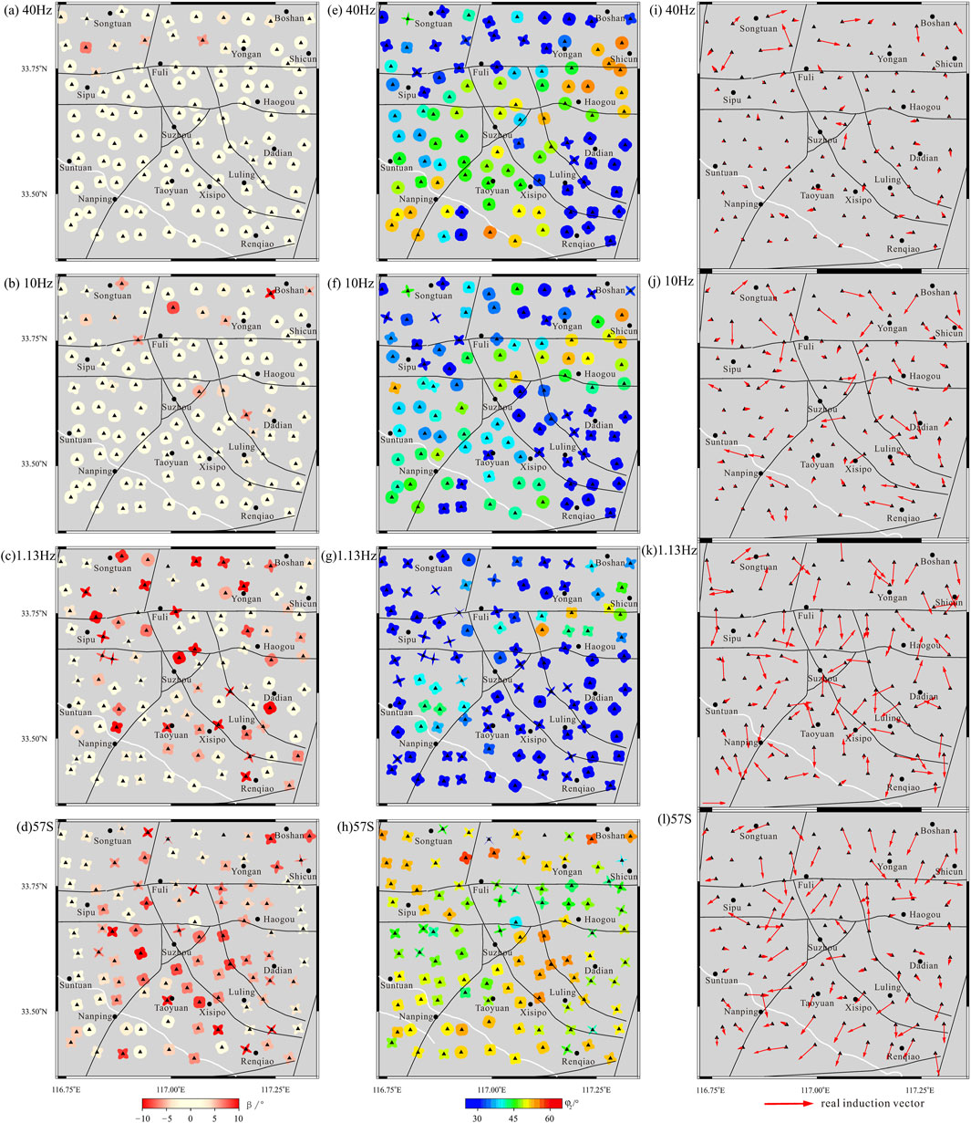
Figure 4. Phase tensor and real induction vector. (a–d): Phase tensor skew angle β. (e–h): Phase tensor invariant φ2. (i–l): Real induction vector.

At high frequencies (corresponding to shallow depths), most phase tensor ellipses appear nearly circular, and the amplitudes of the real induction vectors are relatively small, indicating that the shallow subsurface is predominantly one-dimensional. This reflects the widespread distribution of Cenozoic sedimentary strata across the shallow portions of the study area (Figures 4a,b). In the southeastern and northern parts of the region, slightly elevated skew angles (β) are observed, but they generally remain below 5°. Near fault zones, where β is low, the orientation of the major axis of the phase tensor ellipse is generally aligned with the fault trend, while the real induction vector is oriented perpendicular to the fault. In contrast, at low frequencies (corresponding to greater depths), most skew angles (|β|) exceed 5°, indicating pronounced three-dimensionality and structural complexity at depth (Figures 4c,d). The real induction vectors also exhibit larger amplitudes and lack consistent directionality, further supporting the interpretation of a complex 3D resistivity structure in the deep crust (Figures 4k,l).

Across the overall frequency range from high to low, the distribution of φ₂ reveals high-value areas trending NE–SW at shallow depths, corresponding to the widespread Cenozoic sedimentary strata exposed at the surface, roughly coinciding with the Suzhou-Haogou Basin (Figure 4i). The real induction vector amplitudes in these areas are small, indicating a relatively homogeneous, one-dimensional medium. In contrast, low φ₂-value anomalies appear in the southeastern and northern parts of the study area, suggesting slightly higher resistivity values likely due to the exposure of Paleozoic bedrock. The high-resistivity anomalies in the southeast may further reflect the shallow burial depth of older strata. Notably, the real induction vectors show slightly larger amplitudes in the northwestern shallow region, indicating lateral electrical heterogeneity (Figure 4i).

At depth in the middle and upper crust, resistivity values are generally high, with localized high-conductivity anomalies persisting northeast of Haogou and southwest of Suzhou; however, these anomalies are considerably smaller in scale compared to those at shallower depths (Figures 4f,g). In the middle to lower crust, resistivity values gradually decrease, and a prominent high-conductivity anomaly is observed south of the Subei Fault, while the northern side exhibits relatively higher resistivity (Figure 4h). The real induction vectors north of the Subei Fault predominantly point southward, whereas those in the southern part of the study area point southwest, consistent with the φ₂ distribution (Figure 4l). These observations suggest that the deep structure of the study area is roughly delineated by the Subei Fault, marking significant contrasts in physical properties across the fault boundary.

Statistical imaging using multi-site, multi-frequency tensor decomposition enables analysis of variations in the principal electrical axes of tectonic structures with depth, based on frequency distribution cloud maps. This approach helps identify changes in the geometric features of geological structures at different depths and facilitates exploration of the relationships and integration between deep and shallow tectonic units (McNeice and Jones, 2005).

The full-frequency rose statistic plot for all sites in the study area reveals that the dominant orientation of the electrical spindles trends NE (or NW) (Figure 5a). The frequency distribution cloud plot illustrates how these electrical spindles vary with frequency, reflecting their distribution at different depths (Figure 5b). The data are divided into four frequency bands: the first band (80–4 Hz), the second band (4–0.5 Hz), the third band (0.5–0.003 Hz), and the fourth band (0.003–0.00035 Hz). Figures 5c–f present rose diagrams for each band. In the first band, representing shallow depths, the dominant direction of the electrical principal axis is NE (or NW), with occurrences of NEE (NNW) as well, consistent with the primary orientation of surface fractures in the study area. In the second band, corresponding to medium depths, the dominant spindle direction shifts to NEE (or NNW). At greater depths, represented by the third frequency band, the dominant orientation concentrates around NNE (or NWW). The fourth band, representing the deepest structures, exhibits a more dispersed distribution, roughly dominated by NNE (or NWW). This dispersion likely reflects the three-dimensional complexity of the deep tectonic structures, consistent with previous analyses.

Figure 5

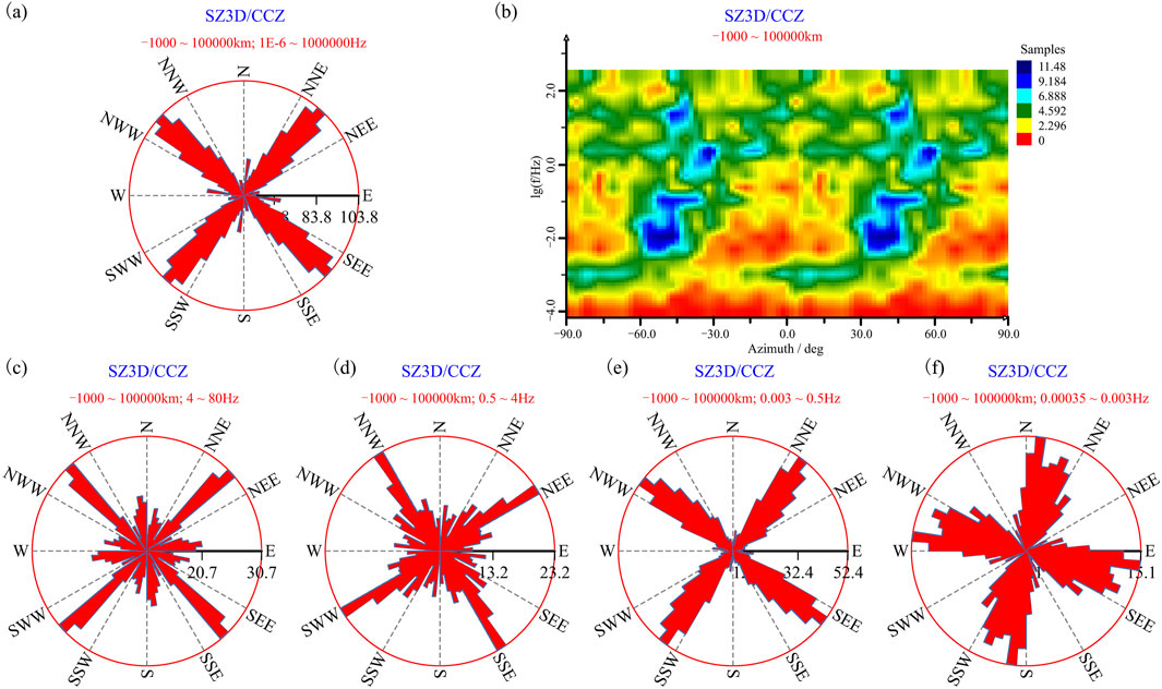
Figure 5. Statistical images of geoelectrical strikes with multi-site, multi-frequency tensor decomposition. (a): Rose diagram for all sites and all frequencies data; (b): Frequency-based cloud diagram for all sites and all frequencies data; (c): Rose diagram for 80–3 Hz band data; (d): Rose diagram for 3–0.05 Hz band data; (e): Rose diagram for 0.05–0.0025 Hz band data; (f): Rose diagram for 0.0025–0.00015 Hz band data.

The qualitative analysis of the geomagnetic observation data provides initial insights into the structural characteristics of the study area. However, obtaining a realistic and reliable subsurface model requires conducting a comprehensive 3D geomagnetic inversion.

3 The 3D inversion and results

3.1 Inversion

The 3D magnetotelluric inversion was performed using the ModEM module embedded in the toPeak 2.0 software platform (Newman and Alumbaugh, 2000; Egbert and Kelbert, 2012; Kelbert et al., 2014). The inversion algorithm is based on the standard minimum-structure nonlinear conjugate gradient method. To construct the initial model, we applied an impression and iterative reconstruction inversion method based on impedance and multiple iterations, which effectively reduces the dependence of the final result on the initial model (For detailed information, see Supplementary Material 1.1, 1.2). During the inversion process, the initial regularization factor was set to 1000 and was reduced by a factor of 5 whenever the decrease in data misfit became insufficient. A total of 100 magnetotelluric (MT) sites were used, and data from 31 frequency points ranging from 320 Hz to 0.000092 Hz were selected. Given the minor topographic variation across the study area, topography was not included in the inversion. Apparent resistivity and phase data from both XY and YX modes were utilized. The core computational domain employed a uniform grid of 1.4 km × 2.1 km, with lateral boundaries extended outward by a scale factor of 1.65. Vertically, the grid began with a 50 m thickness and was extended using segmented scale factors: 1.2 above 1 km, 1.1 between 1 and 5 km, 1.05 from 5 to 50 km, 1.1 from 50 to 150 km, and 1.2 from 150 to 800 km.

The final mesh comprised 125 × 125 × 82 cells (including seven air layers), totaling 1,281,250 cells and covering an area of 2300 km (E–W) × 1250 km (N–S) × 800 km in depth. In 3D MT forward modeling, the top boundary was treated as a far-field open boundary with constant field components (set to 1). The lateral boundaries, due to sufficient model size, were handled using 2D TE/TM forward modeling, while the bottom boundary condition was based on a 1D homogeneous half-space model.

The error floors were set to 3% for apparent resistivity and 0.86° for phase. The final inversion result was achieved after four iterations. The first inversion used a uniform half-space model (100 Ω m) as the starting model, and the subsequent three inversions employed the imprint method, with imprint depths of 30 km, 35 km, and 40 km, respectively. The final model yielded a fitting error of 1.68. Figure 6 compares observed and theoretical response curves for selected sites, demonstrating an excellent data fit.

Figure 6

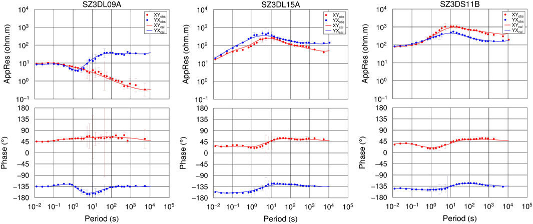
Figure 6. Comparison of observed and modeled response curves. The blue and red dots mark observed responses. The lines mark modeled responses.

3.2 Results

Figure 7 presents slices of the 3D electrical structure model of the study area at various depths. The main tectonic units include the Xuhuai Arcuate Tectonic Structure (XATS) and the Suzhou-Haogou Basin (SHB). At shallow depths (Figure 7a), the XATS is characterized by high-resistivity features, roughly bounded by the western section of the Subei Fault (west of Fuli). However, locally (from Songtuan to Sipu), the high-resistivity zone extends south of the Subei Fault, and the boundary of the eastern section of the XATS (east of Fuli) trends slightly toward the NEE direction. The SHB generally follows a NE-SW trend and exhibits a pronounced low-resistivity anomaly (C1 in Figure 7b), which may extend to about 3 km depth. At the bottom of the upper crust (5–10 km, Figures 7c,d), the area is dominated by widespread high-resistivity features, with localized low-resistivity anomalies in the southwest of Suzhou and northeast of Haogou; these anomalies are significantly smaller in magnitude compared to those at shallower depths. The two principal low-resistivity zones around Suzhou and Haogou are separated by a NW-trending high-resistivity anomaly, R1. From crustal depths downward, a notable low-resistivity anomaly, C2, emerges east of Haogou. As depth increases, this low-resistivity anomaly gradually expands, primarily extending southwestward within the study area (Figures 7e–g). At lower crustal depths (Figure 7h), a broad low-resistivity anomaly, C3, is observed in the southern region, roughly bounded to the north by the Subei Fault.

Figure 7

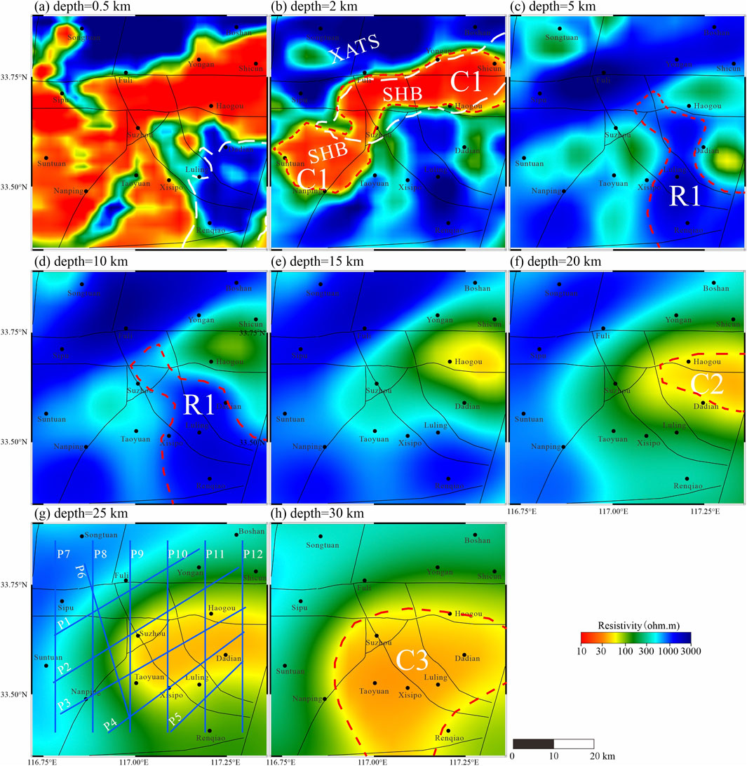
Figure 7. The preferred 3D resistivity models at different depths: (a) 0.5 km, (b) 2 km, (c) 5 km, (d) 10 km, (e) 15 km, (f) 20 km, (g) 25 km, (h) 30 km. XATS: Xuhuai Arcuate Tectonic Structure; SHB: Suzhou-Haogou Basin. The red dotted lines mark the presumed deep electrical boundaries. The white dotted lines mark the range of gravity anomalies. The blue lines mark the location of the profiles in Figures 9, 10.

3.3 Sensitivity tests

In three-dimensional inversion, the results often suffer from significant non-uniqueness, making it essential to evaluate the sensitivity of the derived electrical structure (Burd et al., 2013).

We evaluate the key features of the final inversion model for the study area using forward modeling verification. The resistivity values of the main electrical structures are individually modified to generate corresponding perturbed models. Then, the response data of these perturbed models are calculated through 3D forward modeling and compared with the fitted and observed responses of the original model (For detailed information, see Supplementary Material 1.3, 1.4).

In the 3D electrical structure model of the study area, a prominent NE–SW-trending low-resistivity anomaly (C1) is observed in the upper crust near Suzhou. A NE-trending high-resistivity anomaly (R1) is present between Suzhou and Haogou at the base of the upper crust. Additionally, a low-resistivity anomaly (C2) occurs in the southeastern part of the study area within the middle crust, while a low-resistivity anomaly (C3) is identified in the southern region at lower crustal depths. These electrical anomalies are critical for understanding the crustal deformation mechanisms in the region; hence, sensitivity tests were conducted to evaluate their reliability.

We modified the resistivity in the region of the low-resistivity anomaly C1 to match the resistivity of the surrounding rock within the depth range of 1–3 km. Figures 8a,b illustrate schematic views of the original and perturbed models at a depth of 2 km. A 3D forward simulation of the modified model was performed to obtain the theoretical response curves and fitting errors of the perturbed model. The total fitting error increased from 1.68 in the original model to 4.67 in the perturbed model. Figure 8c shows the spatial distribution of the fitting error difference between the original and perturbed models. It is evident that several sites near the low-resistivity anomaly C1 exhibit significantly worsened fitting errors in the perturbed model. The response curves at typical measurement points for the modified model deviate markedly from the observed data beginning at high frequencies (Figure 8d). These results indicate that the low-resistivity anomaly C1 is well constrained by the observational data and is reliable in the final model. Similarly, sensitivity tests were conducted on the high-resistivity anomaly R1, as well as the low-resistivity anomalies C2 and C3 (see Supplementary Material). The results confirm that these individual anomalies are also constrained by the data and reliable in the final model.

Figure 8

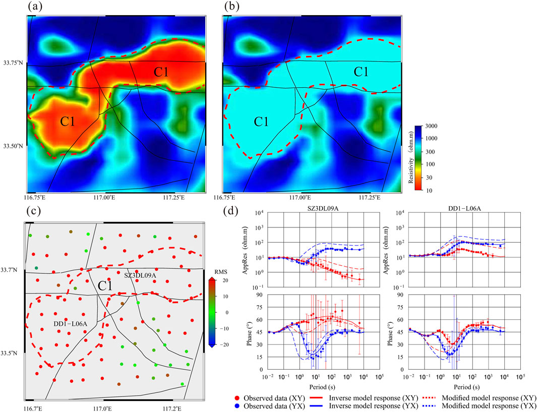
Figure 8. Sensitivity test for the conductive structure C1. (a): The original model; (b): The perturbed model; (c): Map of the ΔRMS at each station; (d): Model response of the perturbed model at some typical stations. The red dotted lines mark the range of C1 at a depth of 2 km.

4 Discussion

To better interpret the electrical structure, we compiled the physical properties of the main rocks and minerals in the study area (Wang et al., 2021) (Table 1). Statistically, the Quaternary sedimentary strata exhibit the lowest resistivity, followed by Carboniferous and Permian sandstones, mudstones, and argillaceous limestones, which have moderate resistivity values. The Ordovician and Cambrian strata mainly consist of limestone and dolomite, with relatively high resistivity values; notably, the Ordovician strata contain more dolomite and thus have slightly lower resistivity than the Cambrian strata. The Proterozoic strata are predominantly composed of quartz sandstone, limestone, and to a lesser extent dolomite, all characterized by high resistivity values. Among the igneous rocks, diorite shows higher resistivity than granite and is also associated with greater density and magnetization.

Table 1

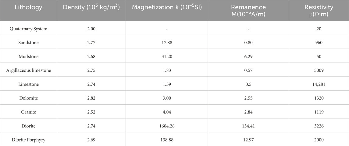
Table 1. Statistics of physical properties of rocks (minerals).

The main tectonic units in the study area are the Xuhuai Arcuate Tectonic Structure (XATS) in the north and the Suzhou-Haogou Basin (SHB) in the south. Near the surface (Figure 7a), the XATS appears as a prominent high-resistivity feature, with only a small low-resistivity area in the northwest, corresponding to the sedimentary strata of the Zhahe syncline core. Significant high resistivity is observed in the southeastern part of the region. The range of the gravitational high-value anomaly (indicated by the white dotted line in Figure 7a) aligns closely with the high-resistivity zones on the electrical structure map. This consistency is mainly due to the presence of limestone, dolomite, and quartz sandstone in this area, which have high density and resistivity values (Table 1), resulting in both high-resistivity and high-gravity anomalies. The remainder of the study area is dominated by extensive low-resistivity features, reflecting the distribution of shallow sedimentary strata. With increasing depth (Figure 7b), the high-resistivity extent of the XATS expands further, and the high-resistivity zone in the southeastern study area extends northwest and southwest. A significant low-resistivity anomaly (C1) trending NEE-SW is evident within the study area. The spatial correspondence between the low-resistivity and low-gravity anomaly zones (white dotted lines in Figure 7b) is even stronger, reflecting the sedimentary strata in the SHB. Overall, the high and low resistivity patterns at shallow depths correspond well with the main structural features: regions with thicker shallow sedimentary strata exhibit low resistivity, while areas with exposed or shallower older strata show high resistivity.

In the upper crust of the study area (Figures 7c,d), most regions exhibit high resistivity characteristics, while low-resistivity zones are primarily found in the eastern part of the study area and the southwestern locality of Suzhou. Resistivity values in these areas are slightly higher than those of the low-resistivity layer at the surface, with the two low-resistivity regions separated by the high-resistivity anomaly R1. As depth increases, the low-resistivity area in the eastern part of the study area expands, whereas the low-resistivity zone in southwestern Suzhou gradually diminishes. In the middle crust (Figures 7e,f), both the amplitude and extent of the low-resistivity anomaly C2 further increase, with its center shifting southward. In the lower crust (Figures 7G,H), anomaly C2 progressively extends southwestward into the low-resistivity anomaly C3. With increasing depth, C3 expands toward the southwest and northwest but remains mainly confined to the southern side of the Subei Fault. Additionally, the greatest sediment thickness in the Suzhou-Haogou Basin (SHB) aligns closely with the upward extension of C3, suggesting that the basin’s formation and evolution may be linked to this low-resistivity anomaly.

From the perspective of the shallow resistivity structure (Figures 7a,b), the Subei Fault generally follows the boundary between high and low resistivity west of Yongan, while to the east of Yongan, it is overlain by low-resistivity sediments. In the upper to middle crust (Figures 7c–f), the eastern section of the Subei Fault appears to roughly align with the boundary between high and low resistivity zones. Therefore, the Subei Fault likely serves as the northern basin-margin fault of the Suzhou-Haogou Basin (SHB), consistent with previous qualitative analyses. Near the surface, the Xinjia Fault controls the southern boundary of the northeastern section of the SHB. At depths of 5–10 km, this fault extends approximately along the southern boundary of the Haogou low-resistivity zone. Below 10 km, the electrical signature of the Xinjia Fault becomes indistinct, suggesting that the fault may be limited to the upper crust.

Based on the distribution characteristics of faults in the study area, several profiles were extracted along the NE and NS directions, respectively (profile locations are indicated by white lines in Figure 7g). The NE-trending profiles primarily analyze the electrical structure associated with NW-trending faults, while the NS-trending profiles focus on EW-trending faults. Additionally, relocated earthquake hypocenters are projected onto these profiles.

Figure 9 illustrates the electrical structure along the NE-trending profile of the study area. The Nanping Fault is nearly vertical at shallow depths but inclines southwestward at greater depths. Its extension is relatively shallow and may be connected to the blind fault Ft6 at depth. The Ft6 fault lies within a low-resistivity zone sandwiched between high-resistivity anomalies and connects at depth with the low-resistivity anomaly C3 in the lower crust. The fault plane of Ft6 is slightly inclined eastward, and given its large scale, it is inferred that Ft6, together with the Nanping Fault, may control the formation and evolution of the southwestern section of the Suzhou-Haogou Basin (SHB). The northern section of the Xisipo Fault is shallowly covered by low-resistivity sedimentary strata and is located within a high-resistivity medium at depth, with weak electrical signatures. The middle section’s shallow depth marks the boundary between high and low resistivity, while at depth it resides within a low-resistivity zone flanked by high-resistivity regions. The fault plane is nearly vertical near the surface but tilts eastward at depth. The southern section’s shallow depth also corresponds to a high-low resistivity boundary, while the deeper part lies within a high-resistivity medium, showing minimal electrical contrast. Similarly, the shallow part of the Dongsanpu Fault is covered by low-resistivity sediments, while its deeper portion lies within a high-resistivity medium, with indistinct electrical characteristics.

Figure 9

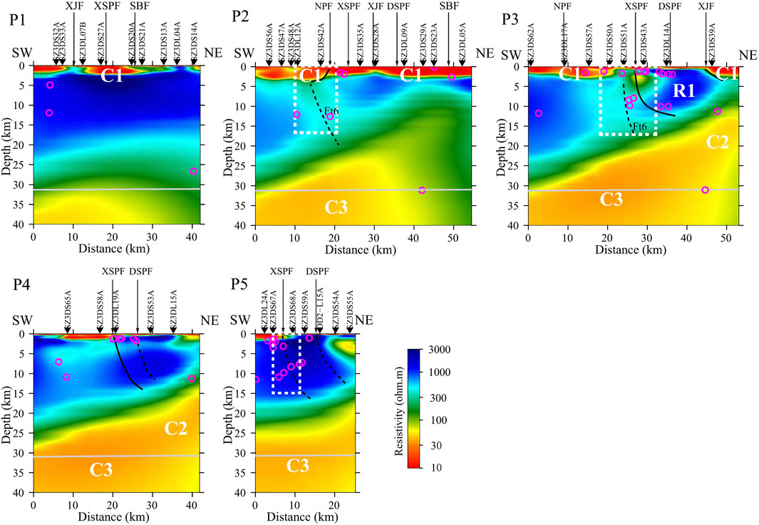
Figure 9. Cross-sections of resistivity model (P1-P5). Locations of these cross-sections are shown in Figure 7G. The white dotted lines mark possible seismic hazard zones. The thin gray line indicates the Moho. The black dotted lines mark presumed faults. The magenta circles mark relocated earthquakes.

Figure 10 displays the electrical structure along the NS-trending profile of the study area. The western section of the Subei Fault delineates the northern boundary of the Suzhou-Haogou Basin (SHB) and exhibits a gently southward-dipping fault plane, while the eastern section is overlain by a low-resistivity layer. At depth, the Subei Fault may connect with the blind fault Ft2. The western section of the Xinjia Fault shows no distinct electrical signature, whereas the eastern section forms the southern boundary of the SHB, with a fault plane dipping northward. Fault Ft2 is situated within the thickest low-resistivity zone of the SHB and links to anomalies C2 and C3, which appear to act as conduits for the upward migration of low-resistivity materials. Given its considerable scale, Ft2 may be the primary controlling fault of the SHB.

Figure 10

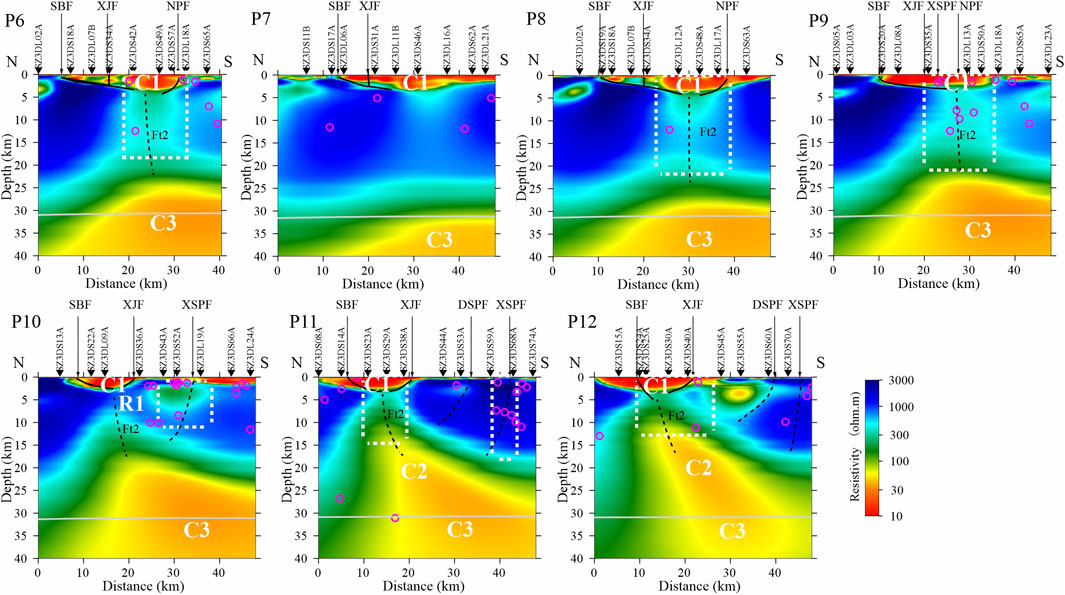
Figure 10. Cross-sections of the resistivity model (P6-P12). Locations of these cross-sections are shown in Figure 7G.

Previous studies on the deep electrical structure of regions with moderate to strong seismicity have shown that low-resistivity zones—flanked by high-resistivity areas and intersected by active faults—are more prone to moderate to strong earthquakes (Becken and Ritter, 2012; Cheng et al., 2019; Sun et al., 2020). High-resistivity zones tend to accumulate significant stress and energy, while active faults provide a tectonic framework for earthquake generation and seismic nucleation. The low-resistivity areas represent relatively weak zones that, under high stress, are the first to exceed their stress limits and undergo rupture, thus acting as seismic hazard zones for moderate to strong earthquakes. Based on this understanding, three seismic hazard zones have been identified along the NE-trending profile of the study area (indicated by white dotted lines in Figure 9), and seven along the NS-trending profile (shown by white dotted areas in Figure 10). These zones are mainly located within the channels uplifted by the low-resistivity anomaly C3. Due to the weaker rock strength in these low-resistivity zones contrasted with the surrounding stronger rock, stress tends to concentrate here. Additionally, frequent minor seismic events and active faults indicate the potential for seismic nucleation and the presence of a deep seismogenic environment. Therefore, future work should prioritize detailed detection and monitoring of these seismic hazard zones, with particular focus on deformation and stress monitoring.

In addition to deep tectonic physical and structural conditions, external driving forces are necessary for the occurrence of moderate to strong earthquakes. Based on the inversion results of the 3D electrical structure model of the study area, combined with insights from related disciplines, we comprehensively analyze the deep seismogenic environment of the Huaibei Plain Fold Belt and discuss the driving mechanisms behind current tectonic deformation. Previous analyses indicate that the potential seismic hazard zones in the Huaibei Plain Fold Belt are closely associated with the deep low-resistivity anomaly C3. Therefore, understanding the nature and possible origin of anomaly C3 is critical for investigating the seismogenic environment in this region.

Deep seismic profiling conducted in 1989 along the Zhengzhou-Lingbi line revealed that the shallow subsurface of the study area consists of low-velocity sedimentary layers, whose morphology aligns with the observed low-resistivity features. The Moho depth contour maps and seismic sounding data from Anhui Province (Li et al., 2006; 2013; 2014; Ai et al., 2007; Shi et al., 2013) indicate minimal variation in the Moho surface depth within the study area, with no evidence of uplift, suggesting that mantle material has not intruded into the crust. Additionally, the Curie depth surface lies between 24 and 25 km (Li and Wang, 2016; Li et al., 2017; Xu Y. et al., 2017; Lei et al., 2024), showing no significant uplift beneath the low-resistivity anomaly C3. This indicates an absence of notable thermal anomalies beneath the study area, implying no current upwelling of mantle-derived thermal material. Geothermal gradient and heat flow distributions (Hu et al., 2000; Tao and Shen, 2008; Jiang et al., 2016; 2019) reveal that values in the study area are lower than those of other basins within the North China Plate, further supporting the lack of significant thermal anomalies. Metallogenic studies have documented Yanshanian hydrothermal-skarn deposits along the Subei Fault (Xu D. R. et al., 2017; Chang et al., 2019; Zhou et al., 2021), indicating that the region associated with the low-resistivity anomaly C3 contains a certain amount of fluid.

Taken together, these observations suggest that the low-resistivity anomaly C3 may represent a remnant of Mesozoic mantle thermal material that has since cooled to a low temperature. However, due to the presence of fluids and significant structural deformation, the current low-resistivity anomaly has developed its observed characteristics. Since there is no evidence of mantle thermal material upwelling beneath the Huaibei Plain Fold Belt, the influence of deep materials on present-day tectonic deformation is likely minimal.

The study area is situated at the junction of the North China and South China plates and is influenced by the Tancheng-Lujiang Fault Zone to the east, resulting in relatively complex tectonic movements. Previous research indicates that from the Archean to the Paleozoic, the lithospheric mantle beneath the North China Plate exceeded 200 km in thickness. However, from the Mesozoic to the Cenozoic, more than 100 km of this lithospheric root was removed, primarily due to the westward subduction of the Pacific Plate and the eastward migration of the Western Pacific Trench. Since the Mesozoic, eastern China has been dominated by NWW-trending extensional tectonics. Partial melting of the subducted Pacific Plate triggered extensive magmatism and volcanism in eastern China, with strong Mesozoic magmatic activity observed along the continental margins of both the North China and South China plates. Despite this, the extent to which Pacific Plate subduction beneath Eurasia currently influences crustal movement and deformation in mainland China remains debated (Wang et al., 2001). Since the Cenozoic, northward subduction of the Indian Plate and its collision and thrusting against the Eurasian Plate, combined with influences from the Siberian Shield and the Eastern Plate, have driven southeastward motion of the eastern Chinese block. The primary forces driving horizontal motion in North China are thought to be the northeastward push from the northeastern margin of the Qinghai-Tibet Plateau and the southeastward shear exerted by the South China Plate (Zhu et al., 2000; Tapponnier et al., 2001). It has also been proposed that current tectonic deformation in eastern China results from westward movement of the North China Block driven by Pacific Plate subduction, coupled with lateral thrusting of the eastern Tibetan Plateau margin against the South China Block along a SEE-trending direction (Huang et al., 2003; Shen et al., 2005). Using focal mechanism data from the study area, the current stress field tensor was obtained through inversion via the grid search method (Wan et al., 2016). The principal compressive stress axis has an azimuth and inclination of 265.9° and 2.2°, respectively, while the extensional stress axis shows an azimuth and inclination of 356° and 3.4°, respectively. Overall, this reflects horizontal compression oriented east-west and horizontal tension oriented north-south (Figure 11). Collectively, these findings suggest that the driving mechanism behind active tectonic deformation in the Huaibei Plain Fold Belt requires further detailed investigation.

Figure 11

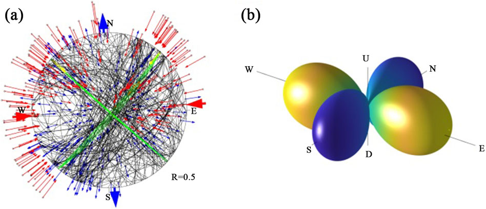
Figure 11. The inverted stress tensor in the study area. (a): The inverted stress tensor in equal-area projection manner. Blue arrows represent the observational slip direction on the “probable fault plane”, and red ones indicate the theoretical slip direction on the “probable fault plane”. The green planes represent the nodal planes with maximum shear stress in confidence level of 95%, and the yellow arrows indicate the slip directions on these planes. Closed curves surrounding S3, S2 and S1 indicate the confidence interval of the compressive, intermediate and extensional stress axis respectively, in confidence level of 95%. E, S, W and N shorthand for east, south, west and north. (b): The stereo representation of the inverted stress tensor. U, D stand for up and down, E, S, W and N mean directions explained as above. Yellow color represents the magnitude and direction of the compressive stress axis, and blue color represents the magnitude and direction of the extensional axis.

5 Conclusion

We acquired high-quality geomagnetic power spectral data through a 3D dense magnetotelluric array survey conducted in the Huaibei Plain Fold Belt. The raw observational data were finely processed using a combination of remote magnetic reference and both Robust and non-Robust geomagnetic time-series processing techniques. Key subsurface structural features were identified by analyzing phase tensors, real induction vectors, and statistical images of geo-electrical strike directions derived from multi-site, multi-frequency tensors. A reliable 3D electrical structural model of the study area was then constructed using 3D magnetotelluric inversion methods. By integrating these results with findings from other geological and geophysical studies, a comprehensive analysis of the deep seismogenic environment and the tectonic deformation driving mechanisms in the study area was performed, leading to the following major insights.

1.The distribution of high and low resistivity at shallow depths in the study area aligns well with major tectonic features. Regions with thicker shallow sedimentary strata, such as the Suzhou-Haogou Basin (SHB), exhibit low-resistivity characteristics, while areas where older strata are exposed or shallowly buried, like the Xuhuai Arcuate Tectonic Structure (XATS), display high-resistivity features. The low-resistivity anomaly C3, which expands progressively with depth, corresponds spatially to the basin’s thickest sedimentary center, indicating a likely correlation between the anomaly and sediment accumulation.

2.The spatial distribution and deep extensions of the main faults in the Huaibei Plain Fold Belt were interpreted. The Subei Fault, Xinjia Fault, and Nanping Fault appear to be the primary faults controlling the boundaries of the Suzhou-Haogou Basin (SHB), with relatively shallow extensions. Basin evolution may be influenced by deep blind faults beneath the basin, which are inferred to be connected to low-resistivity anomalies in the middle and lower crust. These blind faults reside within a weak medium, characterized by low resistivity, and are flanked by higher resistivity zones.

3.A significant low-resistivity anomaly, C3, is present in the lower crust of the study area. Multidisciplinary analyses indicate that C3 results from intense tectonic deformation coupled with the presence of fluids. Currently, there is no evidence of mantle thermal material upwelling beneath the region, suggesting that deep mantle materials have minimal influence on ongoing tectonic deformation.

4.Using the 3D electrical-structure model alongside the regional fault distribution, seismic hazard zones have been delineated. The analysis reveals a deep seismogenic environment in the Huaibei Plain Fold Belt that is capable of generating moderate to strong earthquakes. Nonetheless, the driving mechanisms behind the tectonic deformation require further investigation with the available data.

Data availability statement

The raw data supporting the conclusions of this article will be made available by the authors, without undue reservation.

Author contributions

PL: Visualization, Conceptualization, Validation, Investigation, Writing – review and editing, Formal Analysis, Writing – original draft. JC: Software, Resources, Conceptualization, Data curation, Writing – review and editing, Investigation. SL: Investigation, Writing – review and editing, Resources, Funding acquisition. XC: Software, Supervision, Writing – review and editing, Methodology. YY: Resources, Writing – review and editing, Supervision, Investigation. PS: Investigation, Resources, Funding acquisition, Writing – review and editing. HP: Writing – review and editing, Resources, Investigation. YZ: Investigation, Writing – review and editing. LF: Resources, Writing – review and editing.

Funding

The author(s) declare that financial support was received for the research and/or publication of this article. This research was funded by Anhui Earthquake Administration (20191122, Shuo LU) and the Anhui Key Laboratory of Subsurface Exploration and Earthquake Hazard Risk Prevention (in prep.)(KLB-2025KFQN-003, PL; KLB-2025KFZD-003, PS).

Acknowledgments

We would like to thank the editors and reviewers for their constructive comments and suggestions.

Conflict of interest

The authors declare that the research was conducted in the absence of any commercial or financial relationships that could be construed as a potential conflict of interest.

Generative AI statement

The author(s) declare that no Generative AI was used in the creation of this manuscript.

Any alternative text (alt text) provided alongside figures in this article has been generated by Frontiers with the support of artificial intelligence and reasonable efforts have been made to ensure accuracy, including review by the authors wherever possible. If you identify any issues, please contact us.

Publisher’s note

All claims expressed in this article are solely those of the authors and do not necessarily represent those of their affiliated organizations, or those of the publisher, the editors and the reviewers. Any product that may be evaluated in this article, or claim that may be made by its manufacturer, is not guaranteed or endorsed by the publisher.

Supplementary material

The Supplementary Material for this article can be found online at: https://www.frontiersin.org/articles/10.3389/feart.2025.1615470/full#supplementary-material

References

Ai, Y. S., Chen, Q. F., Zeng, F., Hong, X., and Ye, W. Y. (2007). The crust and upper mantle structure beneath southeastern China. Earth Planet. Sci. Lett. 260, 549–563. doi:10.1016/j.epsl.2007.06.009

CrossRef Full Text | Google Scholar

Becken, M., and Ritter, O. (2012). Magnetotelluric studies at the san andreas Fault Zone: implications for the role of fluids. Surv. Geophys. 33, 65–105. doi:10.1007/s10712-011-9144-0

CrossRef Full Text | Google Scholar

Booker, J. R. (2014). The magnetotelluric phase tensor: a critical review. Surv. Geophys. 35, 7–40. doi:10.1007/s10712-013-9234-2

CrossRef Full Text | Google Scholar

Burd, A. I., Booker, J. R., Mackie, R., Pomposiello, C., and Favetto, A. (2013). Electrical conductivity of the Pampean shallow subduction region of Argentina near 33 S: Evidence for a slab window. Geochem. Geophys. Geosystems 14, 3192–3209. doi:10.1002/ggge.20213

CrossRef Full Text | Google Scholar

Cai, J. T., Chen, X. B., Xu, X. W., Tang, J., Wang, L. F., Guo, C. L., et al. (2017). Rupture mechanism and seismotectonics of the _Ms6.5 Ludian earthquake inferred from three-dimensional magnetotelluric imaging. Geophys. Res. Lett. 44, 1275–1285. doi:10.1002/2016GL071855

CrossRef Full Text | Google Scholar

Cai, J. T., Chen, X. B., Dong, Z. Y., Zhan, Y., Liu, Z. Y., Cui, T. F., et al. (2023). Three-dimensional electrical structure beneath the epicenter zone and seismogenic setting of the 1976 Ms7. 8 Tangshan Earthquake, China. Geophys. Res. Lett. 50, e2022GL102291. doi:10.1029/2022GL102291

CrossRef Full Text | Google Scholar

Caldwell, T. G., Bibby, H. M., and Brown, C. (2004). The magnetotelluric phase tensor. Geophys. J. Int. 158, 457–469. doi:10.1111/j.1365-246X.2004.02281.x

CrossRef Full Text | Google Scholar

Chang, Z. shan, Shu, Q. H., and Meinert, L. D. (2019). “Chapter 6 skarn deposits of China,” in Mineral Deposits of China. Editors Z. S. Chang, and R. J. Goldfarb (Littleton, CO: Society of Economic Geologists), 0. doi:10.5382/SP.22.06

CrossRef Full Text | Google Scholar

Chen, X. B., Zhao, G. Z., and Zhan, Y. (2004). Windows visual integrated system of MT data process and interpretation. Oil Geophys. Prospect. 39 (Suppl.), 11–16 (in Chinese).

Google Scholar

Cheng, Y. Z., Tang, J., Chen, X. B., Dong, Z. Y., and Wang, L. B. (2019). Crustal structure and magma plumbing system beneath the Puer Basin, southwest China: insights from three-dimensional magnetotelluric imaging. Tectonophysics 763, 30–45. doi:10.1016/j.tecto.2019.04.032

CrossRef Full Text | Google Scholar

Egbert, G. D., and Booker, J. R. (1986). Robust estimation of geomagnetic transfer functions. Geophys. J. Int. 87, 173–194. doi:10.1111/j.1365-246X.1986.tb04552.x

CrossRef Full Text | Google Scholar

Egbert, G. D., and Kelbert, A. (2012). Computational recipes for electromagnetic inverse problems. Geophys. J. Int. 189, 251–267. doi:10.1111/j.1365-246X.2011.05347.x

CrossRef Full Text | Google Scholar

Gamble, T. D., Goubau, W. M., and Clarke, J. (1979). Magnetotellurics with a remote magnetic reference. GEOPHYSICS 44, 53–68. doi:10.1190/1.1440923

CrossRef Full Text | Google Scholar

Gu, Q. P., Ding, Z. F., Kang, Q. Q., and Li, D. H. (2020). Group velocity tomography of Rayleigh wave in the middle-southern segment of the Tan-Lu fault zone and adjacent regions using ambient seismic noise. Chin. J. Geophys. 63, 1505–1522. doi:10.6038/cjg2020N0117

CrossRef Full Text | Google Scholar

Gu, N., Gao, J., Wang, B. W., Lu, R. Q., Liu, B. J., Xu, X. W., et al. (2022). Ambient noise tomography of local shallow structure of the southern segment of Tanlu fault zone at Suqian, eastern China. Tectonophysics 825, 229234. doi:10.1016/j.tecto.2022.229234

CrossRef Full Text | Google Scholar

Heise, W., Caldwell, T. G., Bibby, H. M., and Bannister, S. C. (2008). Three-dimensional modelling of magnetotelluric data from the Rotokawa geothermal field, Taupo Volcanic Zone, New Zealand. Geophys. J. Int. 173, 740–750. doi:10.1111/j.1365-246X.2008.03737.x

CrossRef Full Text | Google Scholar

Hu, S. B., He, L. J., and Wang, J. Y. (2000). Heat flow in the continental area of China: a new data set. Earth Planet. Sci. Lett. 179, 407–419. doi:10.1016/S0012-821X(00)00126-6

CrossRef Full Text | Google Scholar

Huang, M., Maas, R., Buick, I. S., and Williams, I. S. (2003). Crustal response to continental collisions between the tibet, Indian, south China and north China blocks: geochronological constraints from the songpan-garzê orogenic belt, western China. J. Metamorph. Geol. 21, 223–240. doi:10.1046/j.1525-1314.2003.00438.x

CrossRef Full Text | Google Scholar

Jiang, G. Z., Tang, X. Y., Rao, S., Gao, P., Zhang, L. Y., Zhao, P., et al. (2016). High-quality heat flow determination from the crystalline basement of the south-east margin of North China Craton. J. Asian Earth Sci. 118, 1–10. doi:10.1016/j.jseaes.2016.01.009

CrossRef Full Text | Google Scholar

Jiang, G. Z., Hu, S. B., Shi, Y. Z., Zhang, C., Wang, Z. T., and Hu, D. (2019). Terrestrial heat flow of continental China: updated dataset and tectonic implications. Tectonophysics 753, 36–48. doi:10.1016/j.tecto.2019.01.006

CrossRef Full Text | Google Scholar

Kelbert, A., Meqbel, N., Egbert, G. D., and Tandon, K. (2014). ModEM: a modular system for inversion of electromagnetic geophysical data. Comput. and Geosciences 66, 40–53. doi:10.1016/j.cageo.2014.01.010

CrossRef Full Text | Google Scholar

Lei, J. S., Zhao, D. P., Xu, X. W., Du, M. F., Mi, Q., and Lu, M. W. (2020). P-wave upper-mantle tomography of the Tanlu fault zone in eastern China. Phys. Earth Planet. Interiors 299, 106402. doi:10.1016/j.pepi.2019.106402

CrossRef Full Text | Google Scholar

Lei, Y., Jiao, L. G., Huang, Q. H., and Tu, J. Y. (2024). A continental model of Curie point depth for China and surroundings based on equivalent source method. J. Geophys. Res. Solid Earth 129, e2023JB027254. doi:10.1029/2023JB027254

CrossRef Full Text | Google Scholar

Li, C. F., and Wang, J. (2016). Variations in Moho and Curie depths and heat flow in eastern and southeastern asia. Mar. Geophys. Res. 37, 1–20. doi:10.1007/s11001-016-9265-4

CrossRef Full Text | Google Scholar

Li, S. L., Mooney, W. D., and Fan, J. C. (2006). Crustal structure of mainland China from deep seismic sounding data. Tectonophysics 420, 239–252. doi:10.1016/j.tecto.2006.01.026

CrossRef Full Text | Google Scholar

Li, Q. S., Gao, R., Wu, F. T., Guan, Y., Ye, Z., Liu, Q. M., et al. (2013). Seismic structure in the southeastern China using teleseismic receiver functions. Tectonophysics 606, 24–35. doi:10.1016/j.tecto.2013.06.033

CrossRef Full Text | Google Scholar

Li, Y. H., Gao, M. T., and Wu, Q. J. (2014). Crustal thickness map of the Chinese mainland from teleseismic receiver functions. Tectonophysics 611, 51–60. doi:10.1016/j.tecto.2013.11.019

CrossRef Full Text | Google Scholar

Li, C. F., Lu, Y., and Wang, J. (2017). A global reference model of Curie-point depths based on EMAG2. Sci. Rep. 7, 45129. doi:10.1038/srep45129

PubMed Abstract | CrossRef Full Text | Google Scholar

Liu, Z. yin, Kelbert, A., and Chen, X. bin (2024). 3D magnetotelluric inversion with arbitrary data orientation angles. Comput. and Geosciences 188, 105596. doi:10.1016/j.cageo.2024.105596

CrossRef Full Text | Google Scholar

Ma, C., Lei, J. S., and Xu, X. W. (2020). Three-dimensional shear-wave velocity structure under the Weifang segment of the Tanlu fault zone in eastern China inferred from ambient noise tomography with a short-period dense seismic array. Phys. Earth Planet. Interiors 309, 106590. doi:10.1016/j.pepi.2020.106590

CrossRef Full Text | Google Scholar

McNeice, G. W., and Jones, A. G. (2005). “Multi-site, multi-frequency tensor decomposition of magnetotelluric data,” in SEG technical Program expanded abstracts, 1996, 281–284. doi:10.1190/1.1826619

CrossRef Full Text | Google Scholar

Meng, Y. F., Yao, H. J., Wang, X. Z., Li, L. L., Feng, J. K., Hong, D. Q., et al. (2019). Crustal velocity structure and deformation features in the central-southern segment of Tanlu fault zone and its adjacent area from ambient noise tomography. Chin. J. Geophys. 62, 2490–2509. doi:10.6038/cjg2019M0189

CrossRef Full Text | Google Scholar

Newman, G. A., and Alumbaugh, D. L. (2000). Three-dimensional magnetotelluric inversion using non-linear conjugate gradients. Geophys. J. Int. 140, 410–424. doi:10.1046/j.1365-246x.2000.00007.x

CrossRef Full Text | Google Scholar

Parkinson, W. D. (1959). Directions of rapid geomagnetic fluctuations. Geophys. J. Int. 2, 1–14. doi:10.1111/j.1365-246X.1959.tb05776.x

CrossRef Full Text | Google Scholar

Patro, P. K., Uyeshima, M., and Siripunvaraporn, W. (2013). Three-dimensional inversion of magnetotelluric phase tensor data. Geophys. J. Int. 192, 58–66. doi:10.1093/gji/ggs014

CrossRef Full Text | Google Scholar

Rong, Z. H., Liu, Y. H., Yin, C. C., Wang, L. Y., Ma, X. P., Qiu, C. K., et al. (2022). Three-dimensional magnetotelluric inversion for arbitrarily anisotropic earth using unstructured tetrahedral discretization. J. Geophys. Res. Solid Earth 127, e2021JB023778. doi:10.1029/2021JB023778

CrossRef Full Text | Google Scholar

Shen, Z. K., Lü, J. N., Wang, M., and Bürgmann, R. (2005). Contemporary crustal deformation around the southeast borderland of the Tibetan Plateau. J. Geophys. Res. Solid Earth 110. doi:10.1029/2004JB003421

CrossRef Full Text | Google Scholar

Shi, D. N., Lü, Q. T., Xu, W. Y., Yan, J. Y., Zhao, J. H., Dong, S. W., et al. (2013). Crustal structure beneath the middle–lower Yangtze metallogenic belt in East China: constraints from passive source seismic experiment on the Mesozoic intra-continental mineralization. Tectonophysics 606, 48–59. doi:10.1016/j.tecto.2013.01.012

CrossRef Full Text | Google Scholar

Sun, X. yu, Zhan, Y., Unsworth, M., Egbert, G., Zhang, H. P., Chen, X. B., et al. (2020). 3-D magnetotelluric imaging of the easternmost kunlun fault: insights into strain partitioning and the seismotectonics of the jiuzhaigou Ms7.0 earthquake. J. Geophys. Res. Solid Earth 125, e2020JB019731. doi:10.1029/2020JB019731

CrossRef Full Text | Google Scholar

Sun, Y. J., Wang, H. B., Huang, Y., Wang, J. F., Jiang, H. L., He, Y. C., et al. (2023). Insight into seismotectonics of the central-south tanlu fault in east China from P-wave tomography. J. Asian Earth Sci. 258, 105722. doi:10.1016/j.jseaes.2023.105722

CrossRef Full Text | Google Scholar

Tao, W., and Shen, Z. K. (2008). Heat flow distribution in Chinese continent and its adjacent areas. Prog. Nat. Sci. 18, 843–849. doi:10.1016/j.pnsc.2008.01.018

CrossRef Full Text | Google Scholar

Tapponnier, P., Xu, Z. Q., Roger, F., Meyer, B., Arnaud, N., Wittlinger, G., et al. (2001). Oblique stepwise rise and growth of the Tibet Plateau. Science 294, 1671–1677. doi:10.1126/science.105978

PubMed Abstract | CrossRef Full Text | Google Scholar

Tian, F. F., Lei, J. S., and Xu, X. W. (2020). Teleseismic P-wave crustal tomography of the Weifang segment on the Tanlu fault zone: a case study based on short-period dense seismic array experiment. Phys. Earth Planet. Interiors 306, 106521. doi:10.1016/j.pepi.2020.106521

CrossRef Full Text | Google Scholar

Tietze, K., Ritter, O., and Egbert, G. D. (2015). 3-D joint inversion of the magnetotelluric phase tensor and vertical magnetic transfer functions. Geophys. J. Int. 203, 1128–1148. doi:10.1093/gji/ggv347

CrossRef Full Text | Google Scholar

Wan, Y., Sheng, S., Huang, J., Li, X., and Chen, X. (2016). The grid search algorithm of tectonic stress tensor based on focal mechanism data and its application in the boundary zone of China, Vietnam and Laos. J. Earth Sci. 27, 777–785. doi:10.1007/s12583-015-0649-1

CrossRef Full Text | Google Scholar

Wang, Q., Zhang, P. Z., Freymueller, J. T., Bilham, R., Larson, K. M., Lai, X. A., et al. (2001). Present-day crustal deformation in China constrained by global positioning system measurements. Science 294, 574–577. doi:10.1126/science.1063647

PubMed Abstract | CrossRef Full Text | Google Scholar

Wang, J. X., He, L. C., and Chan, S. W. (2021). Deep gravity and magnetic field anomalies in the ‌Xuhuai Arcuate Tectonic Structure (Anhui section) and their recognition. Geol. Anhui 31, 40–43.

Google Scholar

Xiao, Q. B., Yu, G., Dong, Z. Y., and Sun, Z. L. (2022). Three-dimensional magnetotelluric inversion considering electrical anisotropy with synthetic and real data. Phys. Earth Planet. Interiors 326, 106876. doi:10.1016/j.pepi.2022.106876

CrossRef Full Text | Google Scholar

Xu D. R., D. R., Chi, G. X., Zhang, Y. H., Zhang, Z. C., and Sun, W. D. (2017). Yanshanian (late mesozoic) ore deposits in China – an introduction to the special issue. Ore Geol. Rev. 88, 481–490. doi:10.1016/j.oregeorev.2017.04.022

CrossRef Full Text | Google Scholar

Xu Y., Y., Hao, T. yao, Zeyen, H., and Nan, F. Z. (2017). Curie point depths in North China craton based on spectral analysis of magnetic anomalies. Pure Appl. Geophys. 174, 339–347. doi:10.1007/s00024-016-1421-x

CrossRef Full Text | Google Scholar

Zhang, Y. Y., Wang, P. J., Chen, X. B., Zhan, Y., Han, B., Wang, L. F., et al. (2022). Magnetotelluric time series processing in strong interference environment. Seismol. Geol. 44, 786–801. doi:10.3969/j.issn.0253-4967.2022.03.014

CrossRef Full Text | Google Scholar

Zhang, J., Jing, Y., Chen, X. B., Cai, J. T., Liu, Z. Y., Huang, X. X., et al. (2025). Research on the three-dimensional electrical structure of the shallow portion of the southern segment of the Red River Fault (Dazhai Village). Earth Planet. Phys. 9, 212–224. doi:10.26464/epp2025020

CrossRef Full Text | Google Scholar

Zhou, J., Jin, C., Suo, Y. H., Li, S. Z., Zhang, L., Liu, Y. M., et al. (2021). Yanshanian mineralization and geodynamic evolution in the Western Pacific Margin: a review of metal deposits of Zhejiang Province, China. Ore Geol. Rev. 135, 104216. doi:10.1016/j.oregeorev.2021.104216

CrossRef Full Text | Google Scholar

Zhu, W. Y., Wang, X. Y., Cheng, Z. Y., Xiong, Y. Q., Zhang, Q., Ye, S. H., et al. (2000). Crustal motion of Chinese mainland monitored by GPS. Sci. China Ser. D Earth Sci. 43, 394–400. doi:10.1007/BF02959450

CrossRef Full Text | Google Scholar