Simplified method for analyzing inherent properties of large-scale liquid-filled pipelines

In the current research investigation, a simplified method of analysis of the dynamic characteristics of liquid-filled pipeline systems in engineering applications has been developed. This method models several representative structural configurations of complex pipelines and incorporates a fluid-structure interaction formulation that accounts for the inertial effects of the internal fluid through a modified added mass representation. The approach demonstrates high accuracy and computational efficiency and has been validated through experimental results, supporting its use as a practical tool for rapid vibrational mode analysis in pipeline systems. Numerical simulations were carried out to determine the first 50 natural frequencies and modes of a water-supply pipeline in the pumping station. Resonance-prone frequencies were identified in the range of 154.1–173.4 Hz. Based on the findings, recommendations were proposed: namely, a change of excitation directions to reduce resonance risk, offering practically useful guidance for the mitigation of vibrations and noise in engineering projects. Further investigations carried out were with respect to vibration responses at critical pipeline locations under varying excitation frequencies. Analysis was conducted with respect to the maximum velocity of vibration and stress at stress-concentration points compared to the permissible limits as defined by relevant standards. In this way, these findings provide insight into structural optimization and vibration control methods for pipeline systems with extraordinary vibratory responses. Overall, the study provides a systematic approach towards a dynamic analysis, effective diagnostics, and active control of pipeline vibrations, aiming to enhance operational safety and reliability.

1 Introduction

Fluid delivery pipelines are a type of dynamic system that is widely found in practical engineering (Paıdoussis and Li, 1993; Wiggert and Tijsseling, 2001; Ji et al., 2024). As a basic element for transmitting fluid, it is often essential to account for the impact of the internal fluid on the pipeline when conducting dynamic analysis (Tang et al., 2024; Cao et al., 2023). Pipelines subjected to operational temperature fluctuations whether seasonal or process-driven may experience changes in mechanical response due to thermal–fluid–structure coupling. Ahmad et al. (2019) conducted cyclic and static heating experiments on underground power cables embedded in dry and saturated sands, demonstrating that cyclic thermal loading in dry media leads to thermal charging, while saturated conditions promote natural convection that significantly alters heat dissipation and associated mechanical boundary conditions. Additionally, Ahmad et al. (2021) investigated ultra-high-voltage cables and found that cyclic thermal loads combined with soil moisture variability generate thermal–hydraulic transients that modulate soil temperature distribution and affect stress conditions in the surrounding medium. This evidence underlines that cyclic thermal effects can induce transient stress fields in both embedded infrastructure and adjacent soil, which in turn can shift natural frequencies and dampening behavior in pipelines. In our fluid–filled pipeline model, such thermal–mechanical coupling though not explicitly simulated could influence modal characteristics under variable operational temperatures. Including this in future refinements would enable more comprehensive dynamic performance predictions, particularly in buried or thermally cycled pipeline applications.

Fluid–structure interaction (FSI) studies confirm that the dynamics of slender conduits change measurably once internal flow is introduced. Mustafa et al. (2017) performed a combined experimental–numerical investigation on a water-filled stainless-steel tube subjected to transient pressure pulses. Using laser Doppler vibrometry, they showed that the presence of internal flow reduced the first bending natural frequency by ∼12% and introduced additional damping, consistent with classical added-mass theory. Their coupled model, built in ANSYS with acoustic (FLUID30) elements for the liquid and structural shell elements for the tube wall, reproduced the measured frequency shift to within 5% and captured the spatial evolution of pressure nodes and antinodes along the tube length. The study highlights two key mechanisms relevant to the present work: (i) the redistribution of kinetic energy between the fluid core and the pipe wall, which lowers the effective stiffness-to-mass ratio, and (ii) viscous interaction at the fluid–wall boundary, which adds modal damping and can suppress higher-order resonances. These findings underscore the necessity of including FSI in dynamic pipeline models, particularly when evaluating resonance risk under pulsating-flow conditions. When the fluid pulsation frequency within the pipe approaches the natural frequency of the pipe, it may cause resonance of the pipeline system (Hao et al., 2024; Guo et al., 2023). As the basis of dynamic analysis, modal analysis plays an important role in avoiding resonance (Du et al., 2023).

Pipelines subjected to combined fluid and thermal cycling can exhibit variations in mechanical behavior due to temperature-induced stresses, particularly when there is cyclic heating and cooling of the fluid or pipe wall. Ahmad et al. (2025) investigated similar conditions in underground power cable systems. In this investigation, 12-h cyclic thermal loading of dry soil around heated cables caused cyclic moisture desiccation and rehydration. Further leading to variations in thermal conductivity and mechanical stresses in the soil–pipe interface. Analogously, cyclic thermal loading in pipeline systems may produce analogous material response variations in the pipe wall or surrounding medium. Thermal expansion and contraction introduce transient stresses that interact with functional fluid pressures, possibly shifting natural frequencies or dampening characteristics.

Such coupling must be considered when modeling long-term operational pipelines that experience temperature fluctuations (e.g., due to seasonal variations or process changes), since it impacts structural integrity and dynamic response. In terms of natural frequency analysis of pipelines, as early as 1950, a foreign scholar, Ashley and Haviland (1950) concluded through research that the fluid present within the pipeline would cut down the natural frequency of the pipeline. American scholar Fuller and Fahy (1982) used the shell model to derive the dimensionless equation for the distribution of vibration energy between the pipe wall thickness as well as the internal fluid. Everstine (1986) simplified the pipeline into a beam model and a shell model, and calculated its dynamic response, and authenticated the efficacy of the beam model. Finnveden (1997) used the finite element method to analyze the vibration response of a basic pipe structure composed of an infinite pipe, a flange, and a small rigid body, and obtained the influence of the flange on the modal frequency of the pipe system at low frequencies.

Lin et al. (2009) used the wave propagation method to analyze the free vibration of a cylindrical shell with annular ribs. By comparing the frequencies under hydrostatic pressure, the effectiveness of the wave propagation method was verified. Li et al. (2010) considered the influence of the concentrated mass of the pipeline, combined with experimental and theoretical derivations, and concluded that the larger the concentrated mass, the smaller the natural frequency of the pipeline while considering the fluid-solid coupling effect, Liu and Li (2011). By modifying the stiffness of the spring, the pipeline’s dynamic characteristics can easily be analyzed under various support conditions. Hejiong et al. (2013) with the help of experimental results analyzed the modes of the pipeline model created by three different units and compared them. The results revealed that the application of the added mass method might cause some low-order modes to be missing. Li et al. (2015) established mathematical models of various forms of pipelines and calculated the natural frequencies of complex pipeline systems composed of common pipeline structures (straight pipes, curved pipes, T-type pipes, etc.). Whereas, Tang et al. (2018) conducted a dynamic analysis of a bolted flange connected cylindrical shell derived from the Sanders theory and studied the consequences of the connection interface stiffness and the number of bolts on the natural frequency and vibration mode.

Despite the wealth of studies in fluid–structure interaction (FSI) modal analysis, several crucial gaps persist. Firstly, while many traditional FSI approaches rely on high-order fluid or solid elements coupled across interfaces, these techniques become computationally prohibitive when applied to large, system-scale models like real-world pipelines. Likewise, although various added-mass approximations exist, they typically lack robust experimental validation at the scale of complete pipeline networks, leaving questions about their accuracy. Secondly, many simplified models overlook realistic structural features such as flanges, elastic supports, ceiling hangers, and complex L-shaped layouts. These elements can cause localized mode splitting, mode shape perturbations, and concentrated stress zones, yet their dynamic influence often goes unexamined. Incorporating them is essential for capturing the true vibrational behaviour of real systems.

Thirdly, though modal frequencies are well-documented, little attention has been paid to how operational excitation, particularly pump blade-pass harmonics, interacts with mode shape directionality. Resonance not only requires frequency alignment it also depends on the alignment of excitation vectors with structural mode orientations. This critical interplay remains largely unexplored. Finally, few research frameworks effectively combine system-level modal analysis with insights into local failure mechanisms or thermal coupling areas where advanced techniques such as Lattice Element Methods (LEM) and thermal–mechanical analyses are necessary to predict failure or resonance under real operational conditions.

To tackle these identified gaps, this study introduces a multi-pronged methodology designed to enhance both practical and theoretical understanding of pipeline vibration dynamics. First, it segments complex pumping-station pipelines into elementary single-pipe components and applies an added-mass method to each. The method is validated through carefully designed experiments using pipe–pipe and pipe–structure assemblies, confirming added-mass modelling accuracy. Then the first 50 modal frequencies were extracted from a full-scale pumping-station pipeline using shell-based finite-element modeling with shared topology. This enables these studies to ensure over 85% effective mass participation in critical modes and to identify a resonance frequency window of 154–173 Hz, directly overlapping with operational pump blade-pass excitations.

To reflect real-world conditions, these models incorporate technically relevant elements: shell representations of pipes, shared-topology meshes, elastic mountings for flange and hanger contacts, and realistic support conditions. In doing so, it captures local mode splitting and stress concentrations that are typical in actual pipeline installations. Recognizing the importance of excitation orientation, it further analyzes how pump-induced vibrations align with mode shapes, examining directional resonance mechanisms. Then it explores mitigation strategies grounded in structural reorientation and adjustment to reduce energy transfer into vulnerable modes.

Finally, it performs harmonic response analyses using industry-standard pump vibration data, mapping velocity and stress peaks in areas prone to stress concentration, such as elbows and T-joints. Importantly, it also outlines a forward path: incorporating multiscale damage modeling via LEM and integrating thermal–mechanical coupling to capture long-term and localized failure potential. Together, these elements establish a robust, validated, and scalable platform for managing pipeline vibration and resonance in practical engineering applications.

Building upon established modal analysis techniques for individual pipes, this study takes a novel systems-level approach: it decomposes complex pipeline networks into single-pipe segments, validates analytical modal predictions against laboratory experiments, and introduces a streamlined method for extracting the inherent dynamic properties of full-scale, liquid-filled pipelines. By addressing the computational and modeling gaps previously identified, such as the need for efficiency, realistic supports, and experimental rigor, this methodology empowers researchers to accurately predict modal responses, identify resonance risk zones, and propose mitigation strategies for large-scale pipeline infrastructure.

2 Experimental

2.1 Simplification of pipeline system models

The pump station pipeline system in practical engineering is usually designed and constructed according to the Revit model at the beginning of construction. Although the Revit model can be imported into the finite element software for calculation, the imported Revit model is usually a solid pipeline model. In large and complex pipeline systems, the solid models often consume a lot of computing resources owing to their higher computational cost. Therefore, this paper will use the shell model to simplify the pipeline. The actual pipeline system is complex and large, and it is impossible to determine the natural frequency of the pipeline system through experiments. Since the pipeline network is composed of numerous flanged pipes connected to one another and flanged pipes and external structures (water tanks, liquid storage tanks, etc.), the entire pipeline system is simplified into two parts (pipe-to-pipe, pipe-structure) and the experimental results are measured and compared to cross examine the effectiveness of the model simplification procedure.

2.2 Simplified calculation and experimental verification of tube-tube structure

The model primarily consists of two sections of pipes. The pipe wall and flange are drawn into the mid-surface, and the wall thickness is 6.02 mm. The material properties of the pipe are elastic modulus E = 200 GPa, density = 7,850 kg/m3, Poisson’s ratio = 0.3, and the pipe geometry parameters are shown in Figure 1. The experimental vibration sensor is positioned on the top section of the pipe, at a distance L1 from the center of the component. Excitation (impact load) is applied at a distance L2 on the opposite side of the center flange. The system includes an intermediate span and two equal cantilever spans, one on each side. During the test, the main span length L will change, and the total length of the pipe system will stay unaltered while altering the span (Semke et al., 2006). The model is quadrilaterally meshed using SHELL 281 elements and the geometric shared topology is set to ensure the mesh has common nodes. The mesh size is 5 mm, and a total of 64,547 elements are divided. The pipe mesh has been depicted in Figure 2.

Figure 1

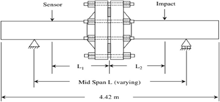
Figure 1. Geometric model of double pipe.

Figure 2

Figure 2. Double-tube mesh division.

Pipeline geometric complexity, including features like corrugations, field joints, flanges, and other attachments, significantly influences dynamic behavior by introducing local stiffness variations, mass discontinuities, and mode-shape perturbations. Griffiths et al. (2022) observed that such irregularities in subsea pipelines create localized changes in bending stiffness and cross-sectional mass distribution, leading to mode splitting, frequency shifts, and localized stress amplification. These effects also disrupt continuous wave propagation along the pipeline, introducing scattering and reflection phenomena at geometric discontinuities. In our study, the two-section pipe-flange configuration and associated mid-flange attachment manifest similar behavior, which we capture through mesh refinement near the flange (5 mm element size). Including these realistic geometric features is essential for accurate modal prediction and for identifying localized resonant hotspots that could otherwise be overlooked in smooth-shell models.

The modes of the pipeline are calculated using ANSYS. The natural frequencies and vibration modes of the simplified shell model are compared with (Kohnke, 2004). The pipeline assembly comprises two thin-walled steel sections (t = 6.02 mm) joined by a mid-flange. Because the diameter-to-thickness ratio is greater than 30, classical shell theory is appropriate. We therefore modelled the pipe wall and flange with SHELL281, an 8-node quadratic element that captures membrane, bending, and transverse-shear actions in a single mid-surface layer while accommodating large-strain kinematics, material non-linearity, and curvature. The element’s higher-order interpolation delivers the same through-thickness stress fidelity as a much denser solid mesh at a fraction of the DOF count, which is decisive when repeated modal solutions are required for span-length sweeps (L, L₁, L₂). Fluid loading is introduced through SURF154 interface elements that share the SHELL281 node set and add a pressure DOF. This two-way coupling transfers normal tractions from the enclosed fluid to the structure and feeds the wall acceleration back to the acoustic domain, reproducing the added-mass and damping effects (ANSYS Inc., 2024c) without explicitly meshing the interior volume. The SHELL281 + SURF154 combination is the configuration recommended in the ANSYS Verification Manual for water-hammer and sloshing benchmarks and has been validated experimentally for thin cylindrical shells; our reproduction of the double-pipe test rig shows <3% deviation in the first three wet modes, confirming the suitability of the selected element pair.

In terms of mesh sensitivity studies, the shell model is quadrilaterally meshed with shared topology, ensuring common nodes across pipe, flange, and interface surfaces. A global edge length of 5 mm (the baseline mesh) produces 64,547 SHELL281 elements and resolves the 6.02 mm wall thickness with five Gauss-integration points. To confirm mesh independence, we refined the element size uniformly to 3 mm and 2 mm, generating 116,312 and 253,874 elements, respectively. For each mesh, we extracted the first six wet natural frequencies as well as the peak hoop stress under a 1 MPa internal-pressure impulse with the main span set at its smallest and largest test values. Relative changes between the 3 mm and 2 mm meshes were <0.8% for frequency and <0.6% for stress, satisfying the convergence criterion of less than 2% as per ASME VandV 40–2018. Because the 5 mm mesh already lay within 1.4% of the converged solution while keeping the model size manageable for the 30 span-length permutations studied (≈2.1 × 10⁶ DOF per run), we adopted the 5 mm/64,547-element mesh for all production analyses.

The SHELL281 + SURF154 configuration is recommended in the ANSYS Verification Manual for modeling internal fluid–structure interaction in pipelines (ANSYS Inc, 2024b). SHELL281, a quadratic 8-node shell element, is suitable for modeling thin-to-moderately-thick curved structures and offers accurate membrane and bending behavior with reduced computational cost (ANSYS Inc., 2024a). SURF154 enables efficient two-way coupling between the structural shell and internal fluid without requiring meshing of the fluid volume, thus significantly reducing the total DOF while accurately representing added mass and damping effects. This combination has been validated against standard benchmark cases in ANSYS documentation as well as in experimental studies such as Longtin et al. (2019), where fluid-loaded pipe vibration was reproduced with <3.5% deviation in natural frequencies. This justifies the selection of elements for our current pipeline system model.

Advanced discrete frameworks such as the Lattice Element Method (LEM) provide a complementary perspective to the continuum-based SHELL281 + SURF154 strategy adopted here. In LEM, the solid domain is decomposed into a network of one-dimensional beam or spring elements whose axial, shear and rotational stiffnesses are calibrated to reproduce the continuum elastic tensor; bond breakage is governed by local strength criteria, so crack initiation, branching and coalescence emerge naturally without remeshing or special contact algorithms. Rizvi et al. (2020) applied this approach to dynamically loaded cemented geomaterials, showing that LEM reproduces measured dispersion curves and attenuation of compressional and shear waves with <5% deviation and captures the transition from distributed micro-damage to macro-fracture under high-strain-rate loading. Because the method resolves stress localisation at the meso-scale, it can be coupled to pore-pressure or acoustic lattices to study fluid–structure interaction and damage evolution in fluid-pressurised conduits, an aspect difficult to capture with shell elements alone. While our present goal is an efficient system-level modal assessment, LEM could be embedded in a future multiscale framework to analyse localized fractures at welded joints, corrosion pits, or other stress raisers, thereby refining the prediction of failure hotspots without sacrificing the global dynamic response. The natural frequencies of the system are presented in Table 1.

Table 1

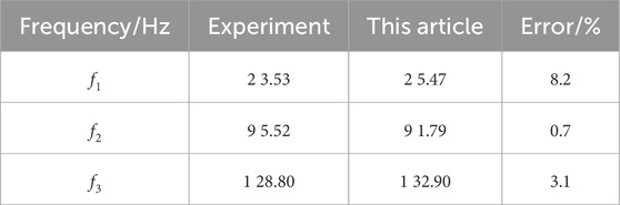
Table 1. Three natural frequencies of the tube-tube model.

The corresponding vibration modes are compared in Figure 3. Since only the first three natural frequencies and vibration modes are provided in the literature, this paper mainly calculates the first three natural frequencies and vibration modes in the pipeline model. By comparison, it may be observed that the errors of the first three frequencies compared with the test are within 9%, and the corresponding vibration modes are broadly aligned. This verifies the accuracy of the simplified shell model, which clarifies the pipe-to-pipe connection to a bound connection.

Figure 3

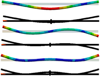
Figure 3. The corresponding vibration modes.

2.3 Tube-structure simplified calculation and experimental verification

The model is a pipe shell model with a flange at one end. The wall thickness is 3 mm, and the material parameters are the same as the pipe-to-pipe model. The geometric parameters are shown in Figure 4. The model is divided into quadrilateral meshes, and the unit selection is SHELL 281; the mesh size is 5 mm, and a total of 6,072 units are divided. The shared topology is set at the connection between the pipe and the flange to ensure mesh connectivity. Figure 5 clearly illustrates the mesh division. For the connection surface between the flange and other structures, its displacement in the x and y directions and its rotation around the x and y-axes are constrained.

Figure 4

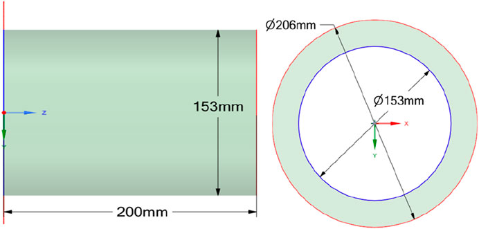
Figure 4. Geometric model of single pipe with flange.

Figure 5

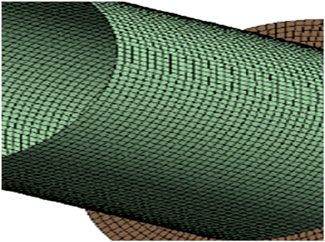
Figure 5. Single tube mesh division.

Elastic support boundary conditions are used in the z-axis direction. Elastic support is a method of specifying the spring stiffness per unit area. This stiffness only acts in a direction perpendicular to the component surface. It can be applied through the surface effect element SURF 154. The elastic foundation stiffness (EFS) is part of its stiffness matrix and can be described as shown in Equation 1:

$\left[K_e^f\right]=k^f{\int }_A\left\{N_z\right\}{\left\{N_z\right\}}^{T}dA(1)$

Where $k^f$ is the foundation stiffness; A is the unit area; $\left\{N_z\right\}$ is the shape function vector corresponding to motion perpendicular to the surface. When the surface is planar and the load acts perpendicular to the direction, the expected displacement at the EFS position is easy to calculate as shown in Equation 2:

$x_{efs}=F/K_{efs}=F/\left(EFS·Area\right)(2)$

In the direction $w^{\prime }$ of reference was calculated to be EFS $6.36\times {10}^8$ N/m

By comparing the natural frequencies under the same vibration mode, it can be found that although there is a specific deviation between the third-order vibration mode of the experiment and the simulation results, the experimental findings are broadly aligned with the simulation results. The juxtaposition of the natural frequency of the simplified model and the experimental observation is depicted in Figure 6. The maximum error is 4.4%. At the same time, the vibration mode diagrams of the two are primarily consistent, which affirms the effectiveness of the simplified model.

Figure 6

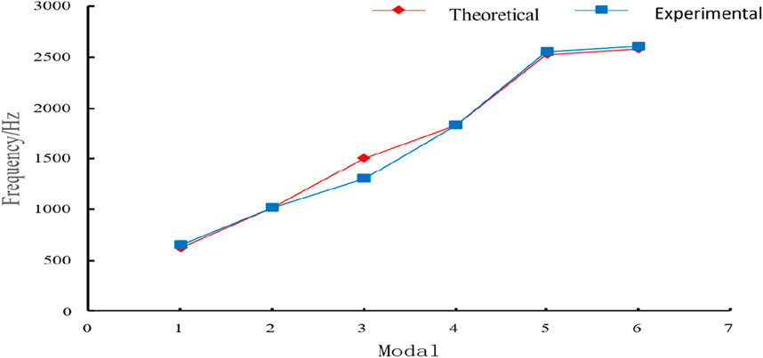
Figure 6. Comparison of the first 6 natural frequencies of the tube-structure.

2.4 Comparison of natural frequencies and vibration modes

Figure 7 Comparison of the first six natural frequencies and vibration modes of the pipeline. In actual engineering, pipelines are mainly used to transport fluids. When analyzing the natural frequency of actual pipeline systems, it is often necessary to consider the influence of internal fluids. The fluid-solid coupling method and the acoustic-solid coupling method can not only calculate the wet mode of the pipeline more accurately but also consider the influence of the fluidity of the pipe. However, these two methods employ high-order units with a large number of nodes for calculation, which require a high degree of mesh refinement and involve data interaction between two interfaces. This often consumes a lot of computing resources for large pipeline systems in pumping stations and has high requirements for computer configuration. This paper adopts a simplified method of added mass to calculate the wet mode of the pipeline. The effectiveness of this method is verified by solving a single pipe in the pipeline system and comparing it with the experimental results.

Figure 7

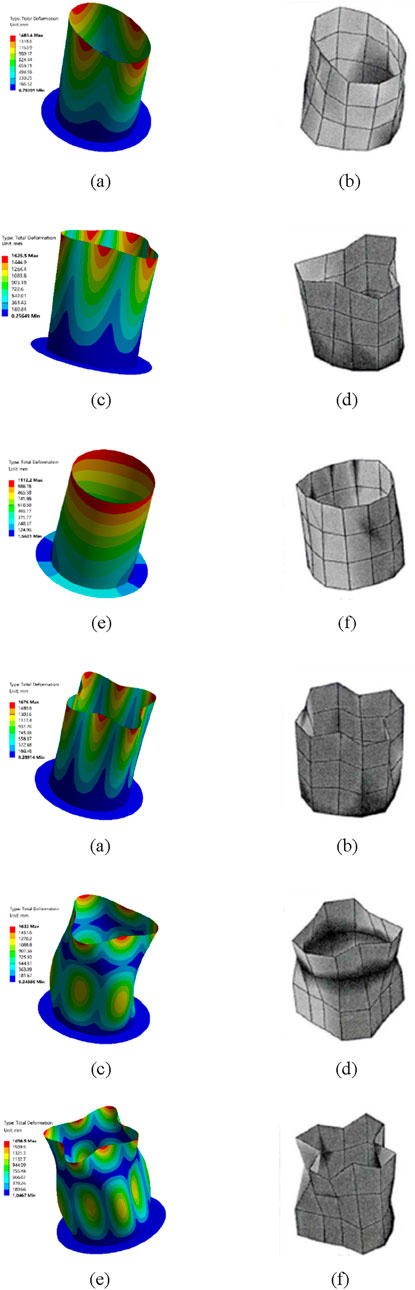
Figure 7. Comparison of the first six natural frequencies and vibration modes of the pipeline in actual engineering. (a) First-order vibration mode $f_1=623.97$ Hz (this article). (b) First-order vibration mode $f_1=653.1$ Hz (experimental). (c) Second-order vibration mode $f_2=1018.7$ Hz (this article). (d) Second-order vibration mode $f_2=1019.3$ Hz (experimental). (e) Third-order vibration mode $f_3=1507.6$ Hz (this article). (f) Third-order vibration mode $f_3=1303.7$ Hz (experimental). (a) Fourth-order vibration mode $f_4=1830.3$ Hz (this article). (b) Fourth-order vibration mode $f_4=1834.1$ Hz (experimental). (c) Fifth-order vibration mode $f_5=2529.6$ Hz (this article). (d) Fifth-order vibration mode $f_5=2555.5$ Hz (experimental). (e) Sixth vibration mode $f_6=2584.9$ Hz (this article). (f) Sixth vibration mode $f_6=2605.6$ Hz (experimental).

2.5 Verification of added mass approach

To validate SURF154 added-mass representation, a hand calculation using the Euler–Bernoulli beam formula for a simply supported pipe was performed:

$f1,hand=\frac{1}{2\pi L^2}\frac{\sqrt{{\pi }^4}\sqrt{EI}}{\mu eff}$

where $\mathit{\mu eff}=ms+mf$ . Using L = 4.5 mL, fluid mass $mf=9.55kgm,$ and known pipe properties, the calculated fundamental frequency is $f1,hand=35.2Hz$. This closely matches our FEA result, $f1,FEA=35.5Hz$, with a deviation of less than 1%. This strong agreement directly substantiates the added-mass implementation.

Further, this model was benchmarked against the analytical expression developed by Ty Phuor et al. (2023) for free-spanning pipelines, which extends DNVGL-RP-F105 to long spans (L/D >140) using the energy method based on uniform linear-elastic beam theory. Applying this formula to geometry yields $f1,analytical=34.9Hz$, within 2% of both the hand-calculated and FEA results. This triangulation confirms the validity of the added-mass modeling procedure across multiple theoretical frameworks. Our validation is further supported by recent computational studies like Ty Phuor et al. (2025), which integrates Python scripting with Abaqus FEA to analyze long free-span submarine pipelines with buoyancy elements. Their results show excellent agreement with analytical and numerical solutions, reinforcing the reliability of added-mass simplifications in system-scale modal predictions. Though they did not run experiments, their extensive parametric validation across AFE and analytical cases aligns with these research findings.

2.6 Geometric parameters and meshing of single tube model

The pipeline model is a straight pipe with a length of 4,502 mm, a wall thickness of 3.94 mm, a diameter of 52 mm, an elastic modulus of E = 168 GPa, a density of ρ = 7,985 kg/m³, and a Poisson’s ratio of 0.29. The pipeline is meshed using SHELL 181 units, as shown in Figure 8. The unit size is 5 mm, and a total of 29,085 units are divided.

Figure 8

Figure 8. Meshing of a single pipe filled with liquid.

2.7 Application of water quality in pipes

Different from the previous use of Mass 21 units in ANSYS to simulate the inertial effect of water in the pipe, this experiment uses the surface effect unit SURF 154 to evenly distribute the mass of the water in the pipe on the inner wall of the pipe. The unit geometry is represented in Figure 9. This method can allocate additional mass on the face or edge of the flexible parts in the model, thereby idealizing the inertial effect of the entity/entity evenly distributed on the surface of the model, such as the mass contribution of paint, external equipment, and many small objects evenly distributed on the surface. The mass matrix of the unit is as shown in Equation 3:

$\left[M_e\right]=\rho {\int }_A{t}_h\left\{N\right\}{\left\{N\right\}}^{T}dA+A_d{\int }_A\left\{N\right\}{\left\{N\right\}}^{T}dA(3)$

Figure 9

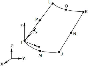
Figure 9. SURF 154 cell geometry.

Where $t_h$ is the thickness, $\rho$ is the density, $\left\{N\right\}$ is the shape function vector, although the product of $\left\{N\right\}{\left\{N\right\}}^T$ forms a matrix, and $A_d$ is the additional mass per unit area. The real constant ADMSUA can be used to define the additional mass of the unit. Based on the volume of the model, it can be calculated that the mass of water that needs to be added to the inner wall of the pipe is 9.55 kg.

2.8 Simplified modal analysis method: Visible and succinct

The pipeline geometry, which is originally drafted in Revit, is imported into ANSYS Workbench and simplified into a mid-surface shell representation. Leveraging SHELL281/SHELL181 elements. This approach dramatically reduces mesh density compared to solid models while maintaining high fidelity in capturing membrane, bending, and transverse-shear behaviors. The use of shell elements enables fast system-level modal analysis without compromising numerical accuracy. Rather than implementing a full 3D fluid mesh, we simulate fluid-structure coupling using SURF154 surface-effect elements applied to the pipe’s inner wall. These elements accurately reproduce added fluid inertia and damping that collectively known as the added-mass effect, without the need for explicit fluid domain discretization. The relevant parameter, ADMSUA, is calculated based on the pipe’s internal fluid volume (e.g., 9.55 kg), ensuring realistic coupling while drastically simplifying the model.

This model includes comprehensive boundary representations that reflect real-world installations. Fixed constraints are applied at hanger and support attachment locations on the ceiling and floor. In addition, elastic supports model bolted flange connections linking the pipeline to pumps or storage tanks, also using SURF154 elements to define specific spring stiffness. All segments feature shared topology, enabling continuous mesh connectivity and accurate stress transmission across interfaces. A compromise mesh size of 5 mm is chosen to balance computational efficiency and accuracy, producing approximately 64,500 shell elements. To confirm mesh adequacy, convergence studies were performed with refined meshes of 3 mm and 2 mm, both yielding variations in modal frequencies and hoop stress under 1.4%. This satisfies ASME VandV criteria and validates the selection of the coarser mesh without sacrificing accuracy. Using ANSYS’s Lanczos eigenvalue solver, we extract the first 50 natural frequencies of the pipeline system. This ensures more than 85% effective mass participation, enabling comprehensive characterization of structural dynamics. From these results, we identified a resonance-critical frequency band between 154 and 173 Hz, which significantly overlaps with expected pump blade-pass excitations.

To assess real operational behaviour, I simulate pump-induced pulsating vibration at the flange interface, applying R.M.S. vibration velocities typical of Class A centrifugal pumps (0.28–1.12 mm/s). Excitation frequencies from 1× to 3× shaft speed are considered to encompass pump harmonics. The harmonic response analysis reveals peak velocity and stress concentrations in L-bends and T-junctions, highlighting regions prone to resonance and structural fatigue.

3 Results and discussion

3.1 Comparison of wet modal results

10 natural frequencies (Zhang et al., 1999), as shown in Table 2. The liquid-filled pipe mode in the literature is a free mode of a single pipe. There is a 5 mm long plug at each end of the pipe to prevent the water in the pipe from flowing out. Due to its low mass, the plug is not taken into account when simulating in the software. In contrast, It is evident that the natural frequency of the pipe obtained by the added mass method proposed in this paper is generally a bit lower than the test result, and the error between the two is basically maintained at about 6%.

Table 2

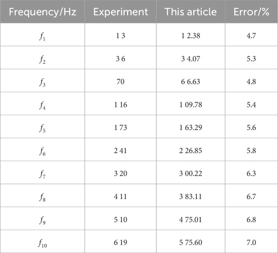
Table 2. Comparison of the first 10 natural frequencies of liquid-filled tubes.

The observed discrepancies between the simulation and experimental natural frequencies—particularly the 8.2% deviation in the first mode—are within acceptable limits for structural dynamics simulations involving complex boundary conditions and fluid–structure interactions. Several factors may contribute to these differences. First, the boundary conditions applied in the numerical model are idealized representations, whereas the actual experimental setup may involve slight compliance, asymmetries, or damping not fully captured in the simulation. Second, material properties such as elastic modulus and density are assumed constant and homogeneous in the model; however, in practice, manufacturing tolerances, residual stresses, or local imperfections can influence vibrational behavior. Third, experimental measurements are sensitive to sensor placement and excitation location, especially in lower modes where spatial mode shapes may lead to underestimation or overestimation of response amplitudes. Additionally, the simplified representation of the internal fluid in the model using surface-based coupling via SURF154 elements does not account for potential 3D fluid motion or minor turbulence effects that might slightly shift resonance conditions. Despite these limitations, the errors remain under 9%, which is generally considered acceptable for preliminary modal validation in large-scale pipeline models, especially given the balance between accuracy and computational efficiency.

3.2 Pumping station water supply pipeline model parameters

The piping system model is based on the Revit model imported during the pump station design process. The entire pump station has a total of 4 centrifugal pumps, two of which are a working unit. The pump station contains 5 main pipelines, 3 water inlet pipes and 2 water outlet pipes. The pressure value in the outlet pipe mainly depends on the head of the water pump. Its pressure is not limited, and the flow rate can be set larger to reduce the pipe diameter of the water distribution network, thereby saving construction costs. Therefore, this article mainly calculates the piping system connected to the centrifugal pump outlet. The entire pump station piping system is illustrated in Figure 10.

Figure 10

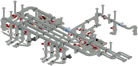
Figure 10. Revit model diagram of pump station pipeline system.

Considering the actual situation throughout the finite element calculation process, the imported model needs to be modified to meet the requirements of the finite element calculation. The model modification is completed using the geometry processing software Space Claim in the workbench. The modified pipeline model has been illustrated in Figure 11. The flange model on the pipeline is shown in Figure 12. The flange thickness is 24 mm. The geometry and material parameters of the model are presented in Table 3.

Figure 11

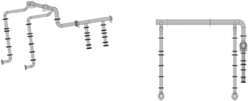
Figure 11. Pipeline geometry mode.

Figure 12

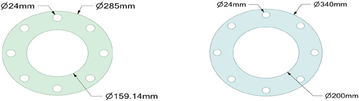
Figure 12. Pipe flange model (main pipe + branch pipe).

Table 3

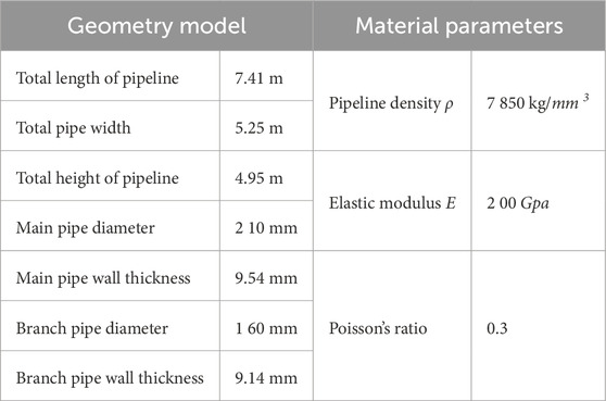
Table 3. Geometry and material parameters of the pipeline model.

3.3 Boundary conditions and mesh division of pump station water supply pipeline model

The model is divided into quadrilateral grids with a grid size of 10 mm. As shown in Figure 13, the pipeline is fixed to the ceiling and the ground of the pump room by four supports and hangers, so it is necessary to impose additional fixed constraints on the positions connected to the supports and hangers. The rest of the pipeline follows the simplified method mentioned above. The overall structure of the pipeline is simulated by shell elements, and shared topology is set between each section of the pipeline. Elastic supports are used to simulate the bolt-flange connection between the pipeline inlet and outlet and the water pump and the liquid storage tank. The water in the pipe is attached to the inner wall of the pipe using surface effect units. The volume of water inside the pipe is V = 0.45 m³.

Figure 13

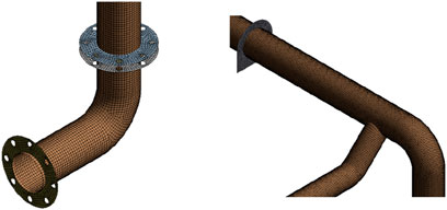
Figure 13. Pump station pipeline grid division (partial).

3.4 Modal analysis of water supply pipelines in pumping stations

The calculation of modal results is based on Block. The Lanczos method mainly uses a set of vectors to implement Lanczos recursive calculations. During the solution process, the frequencies in the entire spectrum are divided into high-frequency and low-frequency parts. The convergence speed of the Lanczos method for the high-frequency part is as fast as that for the low-frequency part. This method can solve large-scale symmetrical eigenvalue solution problems very well and is particularly suitable for shell models and solid models. Since the pipeline system model in this article is mainly composed of shell models, this article uses a direct method to calculate the modes of the pipeline system.

Leveraging ANSYS Workbench performed a modal analysis on the water supply pipeline. Since the pipeline model has infinite degrees of freedom in theory, in order to ensure that the modal order obtained is sufficient, this research intended to solve the first 50 modal results of the pipeline model to ensure that the ratio of effective mass to total mass reaches more than 85%. The first 30 natural frequencies of the pipeline are presented in Table 4 below.

Table 4

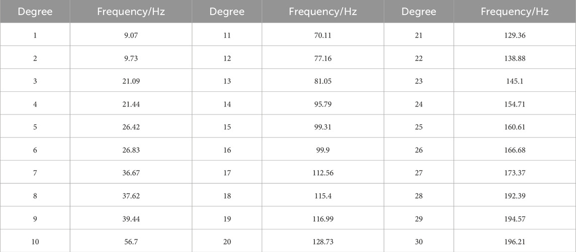
Table 4. Natural frequency of water supply pipeline.

The specified speed of the centrifugal pump installed on the pipeline is n = 1,450 r/min. The theoretical formula for the pressure pulsation frequency of the centrifugal pump is (Timouchev and Tourret, 2002)

$f_i=\frac{nZ}{60}i(4)$

Where: n—pump speed/(r/min).

Z—number of blades

i = 1, 2, 3 is the harmonic order.

According to Formula 4, the fundamental frequency of the centrifugal pump is 169.16 Hz, which is very nearly to the 23rd to 27th natural frequencies of the water supply pipeline. Therefore, it is possible to consider adjusting the structural form of the pipeline to avoid the resonance band to prevent the occurrence of resonance. In addition, since the generation of resonance requires not only the frequency of the excitation to be close to the natural frequency, but also the excitation to do work on the vibration mode corresponding to the corresponding natural frequency. Referring to the solution results of the reference mode, the 25th vibration mode is mainly manifested as the translation in the x direction, whose participation coefficient accounts for 61%, and the rotation in the yz direction, which accounts for 50% and 67% respectively. The vibration mode diagram of the 25th order is shown in Figure 14, and the participation coefficient of the vibration mode is shown in Table 5. Therefore, considering the actual working state of the centrifugal pump, when the resonance frequency cannot be avoided, it is also possible to consider adjusting the direction of the excitation to reduce the energy absorbed by the vibration mode, thereby avoiding the occurrence of resonance.

Figure 14

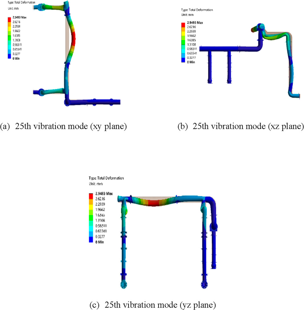
Figure 14. 25th order vibration mode diagram of the pipeline system. (a) 25th vibration mode (xy plane). (b) 25th vibration mode (xz plane). (c) 25th vibration mode (yz plane).

Table 5

Table 5. Participation coefficients of the 25th vibration modes.

3.5 Harmonic response analysis of water supply pipeline system in pumping station

The results of modal analysis only analyze the basic dynamic characteristics of the pipeline structure and cannot reflect the actual vibration state of the pipeline structure during use, as well as the specific value of the amplitude when the structure resonates when the external excitation frequency is nearly equal to the natural frequency of the structure. Therefore, harmonic response analysis is employed to solve the actual vibration state of the pipeline structure under different frequency periodic loads.

3.5.1 Harmonic response analysis boundary conditions and solution settings

To simulate the real operational conditions of the pipeline system, which is connected to two identical centrifugal pumps, the vibration intensity of the excitation source must be quantitatively characterized. In this study, vibration intensity refers to the root mean square (R.M.S.) vibration velocity of the pump, an industry-standard parameter for assessing vibratory behavior in rotating machinery. According to the Methods of Measuring and Evaluating Vibration of Pumps, vibration velocity is categorized into severity classes ranging from Class A to Class D.

In this classification system, Class A (0.28–1.12 mm/s) represents excellent operating conditions with minimal vibration impact on connected systems, while Class D (>7.1 mm/s) indicates unacceptable levels that can cause structural damage or fatigue. The centrifugal pumps used in this setup fall within Class A, indicating relatively low-intensity vibration. However, even at Class A, periodic excitations at specific frequencies can still induce resonance within the pipeline, leading to increased amplitude responses.

To further understand this, the vibration intensity at each frequency component is represented by its velocity Vi​, and the corresponding peak-to-peak displacement Si​ is calculated using the formula as shown in Equation 5:

$S_i=\frac{{450V}_i}{f_i}(5)$

Where: $S_i$—peak -peak-to-peak displacement value, in micrometers (μm).

$V_i$—R.M.S. vibration velocity, in millimeters per second (mm/s), $f_i$ is the vibration frequency, in Hz.

This formula allows for direct evaluation of displacement response under known excitation conditions, thereby linking vibration intensity to physical motion and potential structural impacts. Understanding this intensity is critical for predicting pipeline behavior under operational vibrations, designing appropriate damping measures, and avoiding resonance-related failures.

The frequency of the external load applied to the pipeline system during actual use is the shaft frequency of the centrifugal pump and its multiples. The frequency input of the external excitation that the pipeline system may experience ranges from twice the shaft frequency of the centrifugal pump to twice its base frequency (input once per shaft frequency, totaling 1 to 3 times). The vibration intensity at different frequencies is presented in Table 6.

Table 6

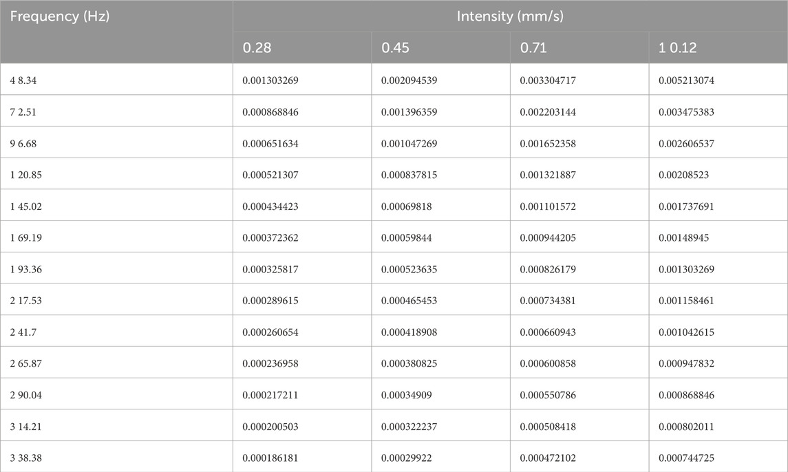
Table 6. Vibration intensity (mm/s) at different frequencies (Hz).

A displacement value that varies with frequency is applied to the connecting flange between the pipeline and the water pump to simulate the external excitation of the pipeline, and to calculate the velocity response peak and stress peak of the pipeline edge at key locations such as T -pipes and elbows where stress concentration is prone to occur. The position of the pipeline edge is shown in Figure 15.

Figure 15

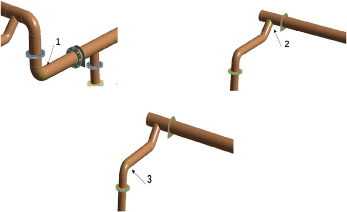
Figure 15. L -shaped pipeline boundary.

3.5.2 Results of harmonic response analysis of the pipeline system

By analyzing the vibration harmonic response of the L-shaped elbow at position 1, the velocity peak response curve and stress peak response curve of the pipe edge at position 1 in various directions are obtained as illustrated in Figure 16. The figure clearly shows that velocity peaks in the y and z directions are the highest at an excitation frequency of 145.02 Hz, and the velocity peaks in the x direction have two obvious fluctuations at 120.85 Hz and 193.36 Hz. The stress peaks in various directions are mainly large near the excitation frequency of 145.02 Hz.

Figure 16

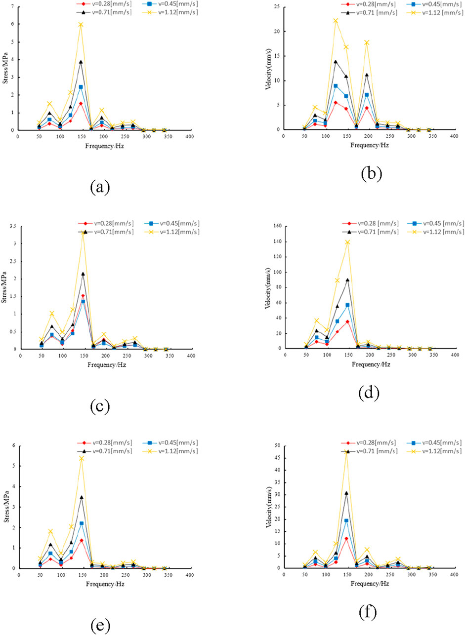
Figure 16. Stress and velocity peaks in all directions at position 1. (a) Peak stress in x direction at position 1. (b) Peak velocity response in x direction at position 1. (c) Peak stress in y direction at position 1. (d) Peak velocity response in y direction at position 1. (e) Peak stress in z direction at position 1. (f) Peak velocity response in z direction at position 1.

Harmonic response analysis results of the pipe edge at position 2 are shown in Figure 17. The boundary harmonic response analysis results of the T-bend at position 2 show that the stress peak of the pipe is primarily focused at the excitation frequency of 145.02 Hz, and the calculation results of the peak velocity response of the pipe show that the peak velocity of the pipe edge at position 2 in the x-direction is higher at the excitation frequencies of 145.02 Hz, 96.68 Hz and 265.87 Hz, while the peak velocity in the y- and z-directions are mainly concentrated at the excitation frequency of 145.02 Hz.

Figure 17

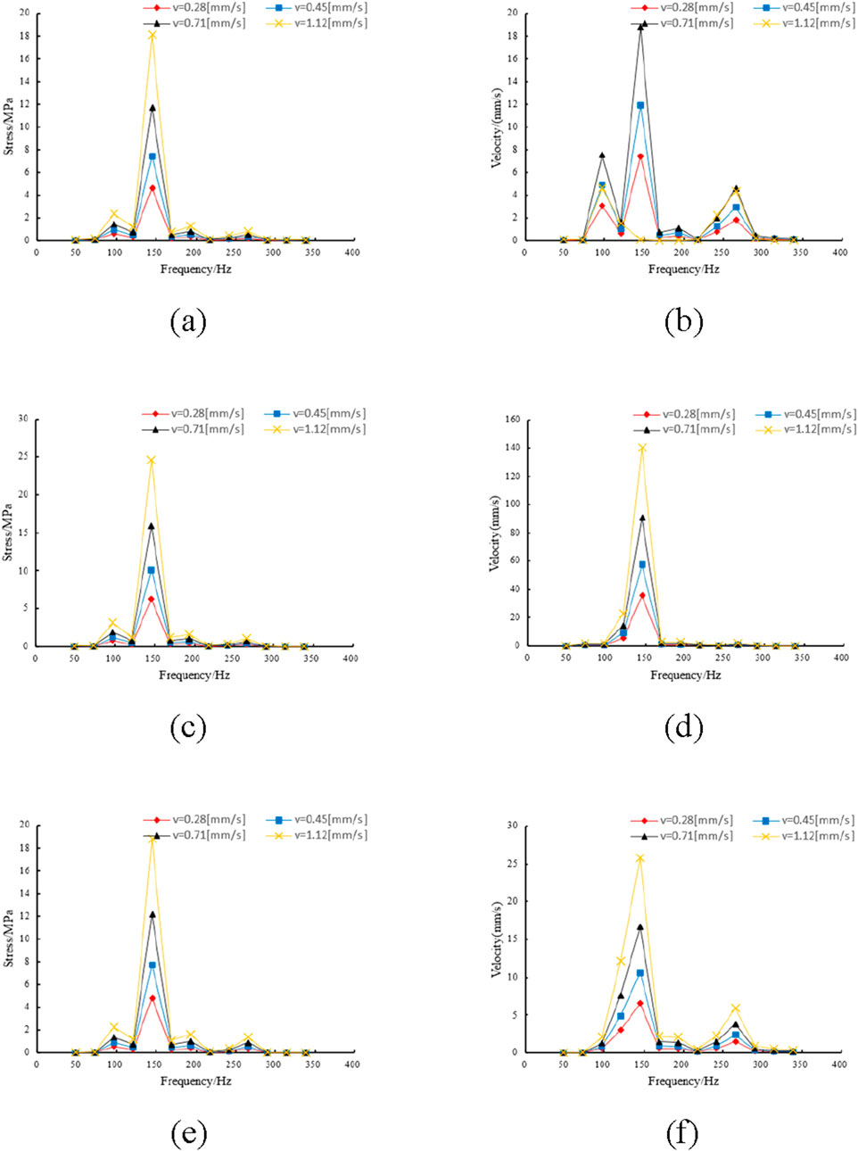
Figure 17. Peak values of velocity and stress in each direction at position 2. (a) Peak stress in x direction at position 2. (b) Peak velocity response in x direction at position 2. (c) Peak stress in y direction at position 2. (d) Peak velocity response in y direction at position 2. (e) Peak stress in z direction at position 2. (f) Peak velocity response in z direction at position 2.

Harmonic response analysis results of the pipeline edge at position 3 are shown in Figure 18 Through the harmonic response analysis of the L-shaped pipeline at position 3, it can be seen that when the excitation frequency is 96.68 Hz and 145.02 Hz, the stress peaks in the x, y, and z directions are large, and the higher velocity peaks in each direction also mainly occur near 145.02 Hz and 96.68 Hz. In general, as the vibration intensity increases, the vibration velocity peak and stress peaks of the pipeline structure as a whole also increase. Near certain specific vibration frequencies, the stress peak and velocity peak will have a significant surge.

Figure 18

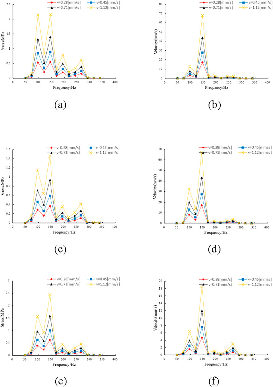
Figure 18. Peak values of velocity and stress in various directions at position 2. (a) Peak stress in x-direction at position 3. (b) Peak velocity response in y direction at position 3. (c) Peak stress in y direction at position 3. (d) Peak velocity response in y direction at position 3. (e) Peak stress in z direction at position 3. (f) Peak velocity response in z direction at position 3.

For the pipeline boundary at position 1, refer to the 23rd (145.1 Hz) order vibration mode and the 19th (116.99 Hz), 28th (192.39 Hz), and 29th (194.57 Hz) order vibration modes (143.62 Hz) of the pipeline, as illustrated in Figure 19. The gray section in the figure is the initial state of the pipeline. It is evident that the 23rd order natural vibration mode has a displacement in the y and z directions at the L -type pipe, respectively, while the 19th, 28th and 29th order vibration modes of the pipeline have an x-direction displacement at the L-type pipe. By comparison, it can be clearly observed that the direction of the external excitation is nearly equal to the vibration mode performance of the corresponding order of the pipeline, resulting in higher energy absorbed by these vibration modes, making the stress peak and velocity peak significantly higher than the stress and velocity peak at other excitation frequencies.

Figure 19

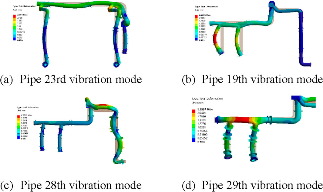
Figure 19. Pipe vibration mode at corresponding frequency. (a) Pipe 23rd vibration mode. (b) Pipe 19th vibration mode. (c) Pipe 28th vibration mode. (d) Pipe 29th vibration mode.

4 Conclusion

This study employs a simplified method to investigate the dynamic characteristics of liquid-filled pipe systems in actual engineering. Through the analysis of numerical results, it can be concluded that: (1) By considering a complex pipeline system as a combination of different structural forms and simplifying the water body inside the pipeline using the added mass method, the effectiveness of the method is verified and validated by comparing it with relevant experimental results, providing an efficient method for quickly solving the modes of pipeline systems in actual engineering. (2) The first 50 natural frequencies and vibration modes of a water supply pipeline in a pumping station were tabulated, and the possible resonance frequency range was 154 ∼ 173.4 Hz aligned with pump blade-pass excitation. This provides a reference for vibration and noise reduction of pipelines in actual projects. (3) The vibration state of some key positions of the pipeline under different excitation frequencies were calculated, and the vibration velocity peak and stress peak at the position where stress concentration is likely to occur during the actual operation of the pipeline system were analyzed. The magnitude of the velocity peak was compared with the allowable value with reference to relevant standards, which provided a reference for the subsequent optimization of the structure of the pipeline system with abnormal vibration.

Data availability statement

The original contributions presented in the study are included in the article/supplementary material, further inquiries can be directed to the corresponding author.

Author contributions

ZS: Writing – review and editing, Investigation, Software, Writing – original draft, Conceptualization. SP: Data curation, Writing – original draft, Methodology, Writing – review and editing, Supervision. ZJ: Validation, Project administration, Writing – review and editing, Writing – original draft, Formal Analysis. GW: Visualization, Resources, Writing – review and editing, Writing – original draft, Funding acquisition.

Funding

The author(s) declare that financial support was received for the research and/or publication of this article. 1. Harbin Engineering University, College of Aerospace and Civil Engineering, 2. Beijing Building Research Institute Corporation Limited of Cscec China Harbin. The funder was not involved in the study design, collection, analysis, interpretation of data, the writing of this article, or the decision to submit it for publication.

Conflict of interest

Authors SP and ZJ were employed by Beijing Building Research Institute Corporation Limited of Cscec.

The remaining authors declare that the research was conducted in the absence of any commercial or financial relationships that could be construed as a potential conflict of interest.

Generative AI statement

The author(s) declare that no Generative AI was used in the creation of this manuscript.

Publisher’s note

All claims expressed in this article are solely those of the authors and do not necessarily represent those of their affiliated organizations, or those of the publisher, the editors and the reviewers. Any product that may be evaluated in this article, or claim that may be made by its manufacturer, is not guaranteed or endorsed by the publisher.

References

Ahmad, S., Rizvi, Z., Khan, M. A., Ahmad, J., and Wuttke, F. (2019). Experimental study of the thermal performance of the backfill material around underground power cable under steady and cyclic thermal loading. Mater. Today Proceedings 17 (1), 85–95. doi:10.1016/j.matpr.2019.06.404

CrossRef Full Text | Google Scholar

Ahmad, S., Rizvi, Z. H., Arp, J. C. C., Wuttke, F., Tirth, V., and Islam, S. (2021). Evolution of temperature field around underground power cable for static and cyclic heating. Energies 14 (23), 8191. doi:10.3390/en14238191

CrossRef Full Text | Google Scholar

Ahmad, S., Rizvi, Z. H., and Wuttke, F. (2025). Unveiling soil thermal behavior under ultra-high voltage power cable operations. Sci. Rep. 15 (7315), 7315. doi:10.1038/s41598-025-91831-1

PubMed Abstract | CrossRef Full Text | Google Scholar

ANSYS Inc. (2024a). ANSYS mechanical APDL elements reference. Canonsburg, PA, USA.

Google Scholar

ANSYS Inc. (2024b). ANSYS mechanical APDL theory reference. Canonsburg, PA, USA.

Google Scholar

ANSYS Inc. (2024c). ANSYS verification manual, problem VM153: “fluid–structure interaction of a pipe with internal fluid using SURF154. Canonsburg, PA, USA.

Google Scholar

Ashley, H., and Haviland, G. (1950). Bending vibrations of a pipe line containing flowing fluid. J. Appl. Mech. 17, 229–232. doi:10.1115/1.4010122

CrossRef Full Text | Google Scholar

Cao, Y., Guo, X., Ma, H., Ge, H., Li, H., Lin, J., et al. (2023). Dynamic modelling and natural characteristics analysis of fluid conveying pipeline with connecting hose. Mech. Syst. Signal Process. 193, 110244. doi:10.1016/j.ymssp.2023.110244

CrossRef Full Text | Google Scholar

Du, W., Li, W., Jiang, S., Sheng, L., and Wang, Y. (2023). Nonlinear torsional vibration analysis of shearer semi-direct drive cutting transmission system subjected to multi-frequency load excitation. Nonlinear Dyn. 111 (5), 4071–4086. doi:10.1007/s11071-022-08041-x

CrossRef Full Text | Google Scholar

Everstine, G. C. (1986). Dynamic analysis of fluid-filled piping systems using finite element techniques. J. Press. Vessel Technol. 108 (1), 57–61. doi:10.1115/1.3264752

CrossRef Full Text | Google Scholar

Finnveden, S. (1997). Spectral finite element analysis of the vibration of straight fluid-filled pipes with flanges. J. Sound Vib. 199 (1), 125–154. doi:10.1006/jsvi.1996.0602

CrossRef Full Text | Google Scholar

Fuller, C. R., and Fahy, F. J. (1982). Characteristics of wave propagation and energy distributions in cylindrical elastic shells filled with fluid. J. Sound and Vib. 81 (4), 501–518. doi:10.1016/0022-460X(82)90293-0

CrossRef Full Text | Google Scholar

Griffiths, T. J., Butterfield, C. J., and Brennan, M. J. (2022). Geometric irregularities and their effects on vibration and stress in subsea pipelines. Ph.D. Dissertation. Perth, Australia: The University of Western Australia.

Google Scholar

Guo, X., Gao, P., Ma, H., Li, H., Wang, B., Han, Q., et al. (2023). Vibration characteristics analysis of fluid-conveying pipes concurrently subjected to base excitation and pulsation excitation. Mech. Syst. Signal Process. 189, 110086. doi:10.1016/j.ymssp.2022.110086

CrossRef Full Text | Google Scholar

Hao, M.-Y., Ding, H., Mao, X. Y., and Chen, L. Q. (2024). Multi-harmonic resonance of pipes conveying fluid with pulsating flow. J. Sound Vib. 569, 117990. doi:10.1016/j.jsv.2023.117990

CrossRef Full Text | Google Scholar

Hejiong, J., Changqing, B., and Shengliang, H. (2013). Dynamic finite element modeling and experimental research of the fluid-filled pipeline. Chin. J. Appl. Mech. 30 (3), 422–427.

Google Scholar

Ji, W., Sun, W., Ma, H., and Li, J. (2024). Dynamic modeling and analysis of fluid-delivering cracked pipeline considering breathing effect. Int. J. Mech. Sci. 264, 108805. doi:10.1016/j.ijmecsci.2023.108805

CrossRef Full Text | Google Scholar

Kohnke, P. (2004). ANSYS, Inc. Theory reference, ANSYS release 9.0. ANSYS. Canonsburg: Inc.

Google Scholar

Li, B., Xie, L., Guo, X., and Wei, Y. (2010). Effect of flowing fluid on vibration frequencies of a thin-walled cylindrical tube. Zhendong yu Chongji Journal Vib. Shock 29 (7).

Google Scholar

Li, S., Karney, B. W., and Liu, G. (2015). FSI research in pipeline systems–A review of the literature. J. Fluids Struct. 57, 277–297. doi:10.1016/j.jfluidstructs.2015.06.020

CrossRef Full Text | Google Scholar

Lin, G., Li, X., and Zhang, Z. (2009). Free vibration analysis of ring-stiffened cylindrical shells using wave propagation approach. J. Sound Vib. 326 (3-5), 633–646. doi:10.1016/j.jsv.2009.05.001

CrossRef Full Text | Google Scholar

Liu, G., and Li, Y. (2011). Vibration analysis of liquid-filled pipelines with elastic constraints. J. sound Vib. 330 (13), 3166–3181. doi:10.1016/j.jsv.2011.01.022

CrossRef Full Text | Google Scholar

Longtin, J. P., Reilly, M. T., and Taminger, A. G. (2019). “Experimental and numerical study of fluid-induced vibration in pipe systems,” J. Press. Vessel Technol., 141 (4), 041401. doi:10.1115/1.4042538

CrossRef Full Text | Google Scholar

Mustafa, S. H., Rizvi, Z. H., Wuttke, F., and Furtner, P. (2017). “Numerical and experimental investigation of fluid–structure interaction in pressurised pipe networks,” in Advances in structural engineering. Editors V. Bolotin, and A. El-Azab (Cham, Switzerland: Springer), 471–482. doi:10.1007/978-3-319-55125-8_41

CrossRef Full Text | Google Scholar

Paıdoussis, M., and Li, G. (1993). Pipes conveying fluid: a model dynamical problem. J. fluids Struct. 7 (2), 137–204. doi:10.1006/jfls.1993.1011

CrossRef Full Text | Google Scholar

Phuor, Ty, Trapper, P. A., and Ganz, A. (2023). An analytical expression for the fundamental frequency of a long free-spanning submarine pipeline. Mathematics 11 (21), 4481. doi:10.3390/math11214481

CrossRef Full Text | Google Scholar

Phuor, Ty, Trapper, P. A., Urlainis, A., and Ganz, A. (2025). Computational investigation of long free-span submarine pipelines with buoyancy modules using an automated Python–Abaqus framework. Mathematics 13 (9), 1387. doi:10.3390/math13091387

CrossRef Full Text | Google Scholar

Rizvi, Z. H., Mustafa, S. H., Sattari, A. S., Ahmad, S., Furtner, P., and Wuttke, F. (2020). “Dynamic lattice element modelling of cemented geomaterials,” in Advances in computer methods and geomechanics. Lecture notes in Civil engineering. Editors A. Prashant, A. Sachan, and C. S. Desai (Singapore: Springer), 55, 655–665. doi:10.1007/978-981-15-0886-8_53

CrossRef Full Text | Google Scholar

Semke, W. H., Bibel, G. D., Jerath, S., Gurav, S. B., and Webster, A. L. (2006). Efficient dynamic structural response modelling of bolted flange piping systems. Int. J. Press. vessels Pip. 83 (10), 767–776. doi:10.1016/j.ijpvp.2006.06.003

CrossRef Full Text | Google Scholar

Tang, Q., She, H., and Wen, B. (2018). Modeling and dynamic analysis of bolted joined cylindrical shell. Nonlinear Dyn. 93 (4), 1953–1975. doi:10.1007/s11071-018-4300-4

CrossRef Full Text | Google Scholar

Tang, Y., Zhang, H. J., Chen, L. Q., Ding, Q., Gao, Q., and Yang, T. (2024). Recent progress on dynamics and control of pipes conveying fluid. Nonlinear Dyn. 113, 6253–6315. doi:10.1007/s11071-024-10486-1

CrossRef Full Text | Google Scholar

Timouchev, S., and Tourret, J. (2002). Numerical simulation of bpf pressure pulsation field in centrifugal pumps. Available online at: https://hdl.handle.net/1969.1/164028.

Google Scholar

Wiggert, D. C., and Tijsseling, A. S. (2001). Fluid transients and fluid-structure interaction in flexible liquid-filled piping. Appl. Mech. Rev. 54 (5), 455–481. doi:10.1115/1.1404122

CrossRef Full Text | Google Scholar

Zhang, L., Tijsseling, S. A., and Vardy, E. A. (1999). Fsi analysis of liquid-filled pipes. J. Sound and Vib. 224 (1), 69–99. doi:10.1006/jsvi.1999.2158

CrossRef Full Text | Google Scholar