 Alejandra I. Sánchez
 Luis A. Gallardo
- Department of Applied Geophysics, Centro de Investigación Científica y de Educación Superior de Ensenada (CICESE), Ensenada, Mexico
Ground penetrating Radar (GPR) is a high-frequency geophysical prospecting method whose signal is affected by dielectric permittivity
1 Introduction
Ground penetrating Radar (GPR) is a non-invasive, high-resolution and highly versatile geophysical prospecting method with diverse applications. The range of radar applications is vast due to their high frequency signal and the wide range of electromagnetic property variations. It is commonly used in geotechnical studies to locate pipes and to determine concrete and pavement conditions in buildings and paved-roads (Cassidy et al., 2011; Zhou and Zhu, 2021), to identify buried objects in forensic geophysics (Schultz and Martin, 2012; Aditama et al., 2015), to locate mines and unexploded ordnances (Steven et al., 2010; Giannakis et al., 2016), in studies of glaciers and permafrost (Hamran et al., 1998; Woodward and Burke, 2007), and to monitor water content in rocks (Klotzsche et al., 2018; Zhou et al., 2019). It is also common to combine the GPR studies with other geophysical or teledetection techniques. For example, to detect deformation zones or subsidence areas (Alonso-Díaz et al., 2023; La Bruna et al., 2024) or in forensic studies (Berezowski et al., 2024; Molina et al., 2024), among other applications.
In archaeology in particular, it is commonly used alone or in combination with other geophysical techniques to search for buried remains, mounds, settlement patterns and ancient buildings (Conyers et al., 2019; Ortega-Ramírez et al., 2020). For instance, coincidences have been found in the results of magnetic exploration and GPR, as in the work of Bianco et al. (2024), who demonstrated the advantages of an integrated interpretation of magnetic and GPR data in archaeological structures. This implies that a magnetic signature exists in both data types, but the underlying magnetic signature in radar data is poorly studied.
It is noticeable that, even in low-frequency electromagnetic (EM) signals, some studies address the importance of magnetic permeability. Pavlov and Zhdanov (2001) analysed the influence of magnetic permeability in TDEM surveys. Noh et al. (2016) evaluated the effects of conductivity and magnetic permeability in the frequency domain controlled-source EM methods. Xiao et al. (2022) studied the resistivity and magnetic susceptibility responses for a 3D Controlled-source audio-frequency magnetotellurics modeling. Heagy and Oldenburg (2023) considered how magnetic permeability contributes to the EM response of a cased well in grounded source EM experiments. Qiao et al. (2025) analysed numerical experiments for a marine magnetotelluric approach considering variations in conductivity and magnetic permeability for 3D modeling. Notably, all of them concluded that the magnetic permeability influences the EM signal.
By being the highest frequency EM technique, it seems reasonable that the three properties must also be considered in radar data. Some authors have studied the effect of
Although the effect of ferromagnetic materials in the GPR signal has been studied, it is still unclear whether this signal is individually distinguishable from those produced by dielectric permittivity and electrical conductivity or not. It is also arguable if magnetic permeability contrast could significantly influence radar signals so as to be noticeable in geophysical data modeling and, ultimately, whether we should be able to infer this magnetic permeability contrast in an inverse problem. We posit that magnetic permeability does affect the observations differently from either electric permittivity or conductivity contrasts and should thus be considered in radar signal modeling and inversion.
This paper analyses the separate and combined influence of the three electromagnetic properties in EM wave propagation at the frequency range of radar signals. The finite-difference time-domain (FDTD) method was implemented to compute the EM response. We compare the computed fields with those from the widely used software gprMax (Giannopoulos, 2005; Warren et al., 2016). We then test if the electromagnetic response of the three properties can be individually distinguished in its propagation through the different media or in its interaction in the medium’s interfaces. We also explore the existence of a response that cannot be reproduced if magnetic permeability variations are ignored.
2 Electromagnetic rock properties
For ground penetrating radar, the equations that govern the electromagnetic phenomenon are Maxwell’s equations, which, in vector notation, are written as:
and
In these expressions,
More commonly,
In a magnetically homogeneous medium, Equations 3,4, can be combined in a single expression, known as the Helmholtz equation for EM propagation:
For a magnetically heterogeneous medium, however, the Helmholtz equation is more complex, and a different scheme is preferred for modeling (Noh et al., 2016; Pavlov and Zhdanov, 2001). Despite this, in electromagnetic modeling, it is common practice to assume either that variations in
The importance of considering magnetic permeability in EM modeling starts from their natural variations in minerals and rocks. It is currently acknowledged that common Earth materials have at least a two-order of magnitude variation in each one of these three electromagnetic properties (Figures 1–3); therefore it seems reasonable that they all may produce an electromagnetic radar response. From the comparative analysis of the summarizing figures, we can remark the following:
1. The material’s dielectric permittivity varies within a much narrower range than conductivity, even under the influence of various fluid (water or air) concentrations. Variations are due to particular sample conditions such as its porosity, the presence of water, its degree of compaction, etcetera.
2. Within their ranges of variation, the presence of water influences notably both the dielectric permittivity and conductivity, whereas magnetic permeability is particularly independent of the water content. In fact, magnetic permeability is the electromagnetic property most influenced directly by mineral composition.
3. Some common target materials in radar exploration, such as basalt, polar ice, etc., can be equivocally characterized by the combined values of the three properties.
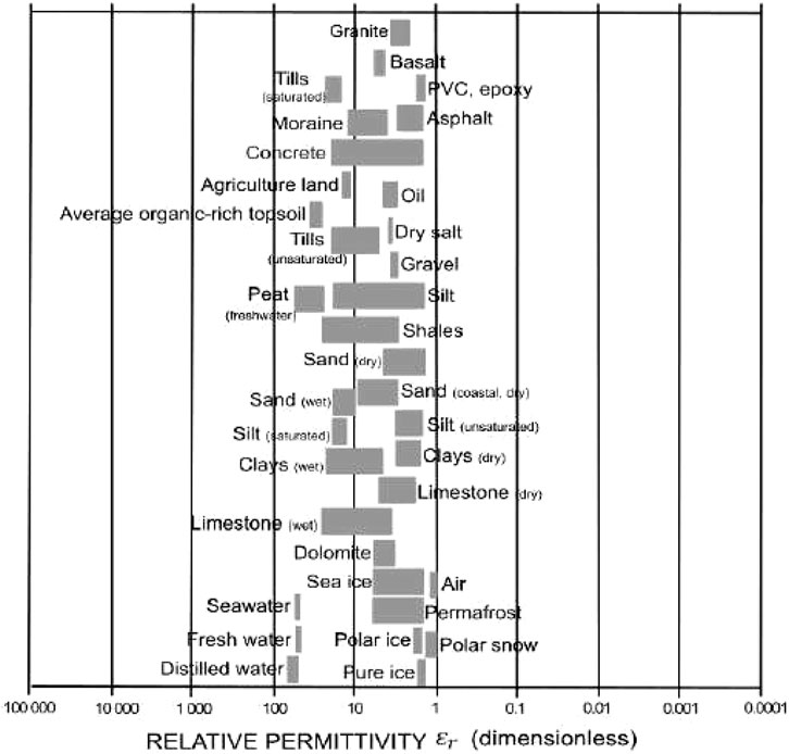
Figure 1. Ranges of relative permittivity values for various materials. Data combined from the compilations of Butler (2012), Reynolds (2011) and Reichard (2020). Note the coincidence of the permittivity values for most materials and that values lie within two orders of magnitude.
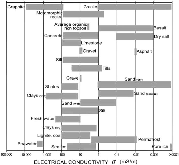
Figure 2. Ranges of electrical conductivity (adapted from Palacky (2012). Note the wide range (eight orders of magnitude) of the conductivity and the significant conductivity variations for individual materials depending on specific material conditions.
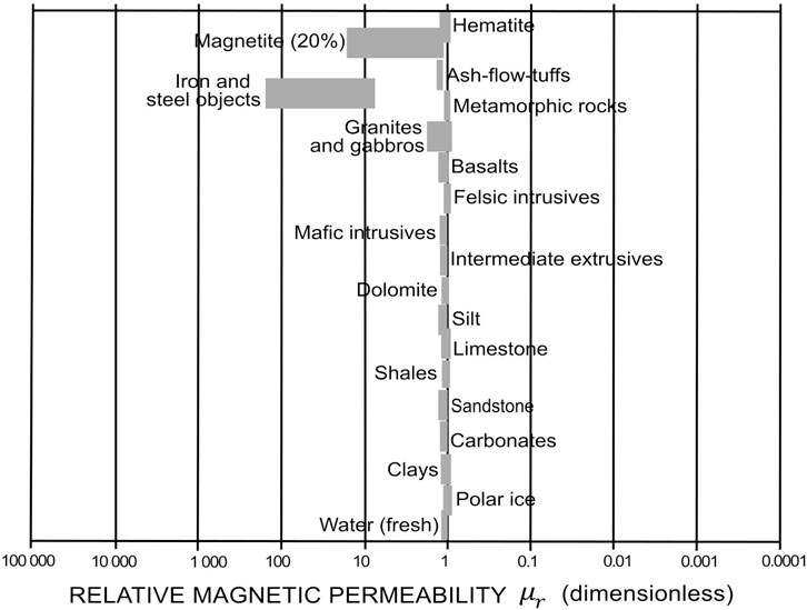
Figure 3. Ranges of relative magnetic permeability adapted from Palacky (2012) and Reichard (2020). Note the three orders of magnitude variations and the marked dominant groups identified as magnetic and non-magnetic.
Conceding that, for Earth materials, heterogeneities in the three EM properties exist and are relevant, we now face the challenge of computing their influence in radar data using directly Equations 1–4.
3 FDTD numerical modeling of radar signals for full heterogeneous models
Finite-difference time-domain (FDTD)
The FDTD method allows solving a coupled set of equations in discrete steps in time and space. It has long been used as a common strategy in seismological modeling, e.g., Virieux and Madariaga (1982), and Komatitsch and Martin (2007), among others. In electromagnetic modeling for geophysical applications, the method has been widely used since the early 90s (Holliger and Bergmann, 1998; Lampe et al., 2003; Cabrer et al., 2022); many of these publications, however, consider
We start our development from Equations 3, 4, using a leapfrog scheme to approximate the time derivatives. The time-step leapfrog scheme was first applied to the solution of Maxwell’s equations by Yee (1966). The Yee cell discretizes the electric and magnetic fields in time and space so that both fields are intertwined. This scheme is known to be second-order accurate, enables computationally efficient time progress, and reduces memory storage.
For the three-dimensional case, Faraday’s and Ampere’s Equations 3, 4 can be expressed as follows:
and
We apply the FDTD scheme in a Yee (1966) grid to Equations 6–11. A schematic diagram of the Yee array is presented in Figure 4 and the relevant update equations for the
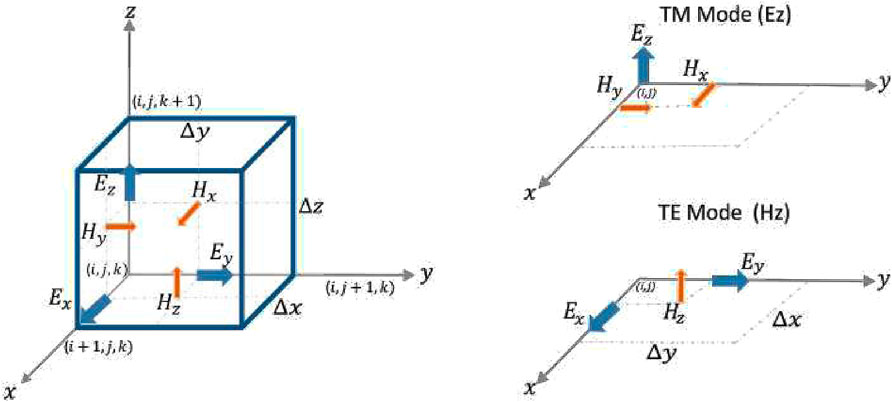
Figure 4. FDTD Yee distribution for a single 3D cell (left) showing the electric (blue) and magnetic (orange) field components. Individual elements for TM and TE modes are shown in the right panel.
and
For a two-dimensional case, the EM fields propagate in two fully-decoupled modes: the transverse electric (TE) and the transverse magnetic (TM) modes.
We will work with the TM mode, where the update equations for
for the electric
and
for the magnetic
Similarly, for the one-dimensional FDTD case, the Maxwell’s equations are reduced to:
and
The above equations represent the necessary components for the 1D and 2D electromagnetic wave propagation for numerical modeling.
In all our experiments, an incoming Gaussian signal with central frequency 200 MHz was used as a source. To have an adequate discrete representation the grid spacing must be sufficiently small to resolve the shortest wavelength. For this, we select 35 point per wave length (min
To reduce spurious waves reflected from the edges of the model we adapt the Perfectly Matched Layer (PML) method for the coupled solution of Ampere’s and Faraday’s laws considering the three EM properties, (e.g., Berenger, 1994). The basic considerations for developing this formulation can be found in Supplementary Appendix A. The adapted PML equations for the corresponding Equations 14, 15, for the two-dimensional TM mode:
where
Similarly, the
with the coefficients:
The Equations 12, 13, which correspond to the 3D formulation, were developed for future work; however, in the following sections, we focus our results on one and two-dimensional models. In this context, the Equations 16–26 were used for modeling the EM propagation. The implemented flowchart of the algorithms is shown in Figure 5.
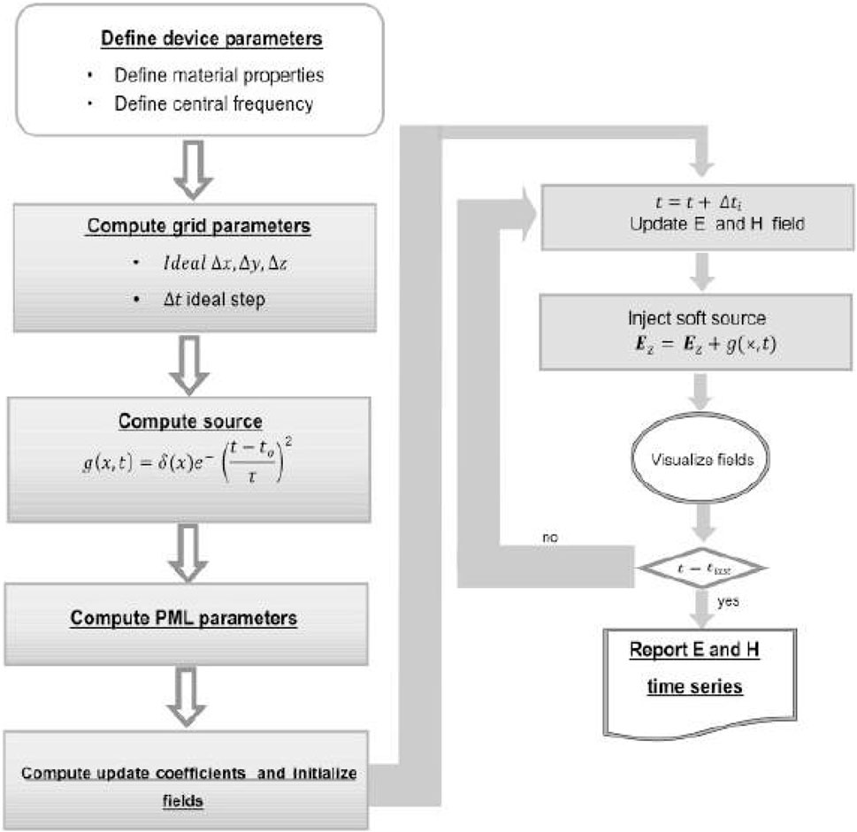
Figure 5. Schematic FDTD algorithm flowchart for numerical modeling.
As a first test to gauge the results obtained from this algorithm, we compare the fields computed for a homogeneous medium with those of the well-known software gprMax (Warren et al., 2016). For this experiment we set
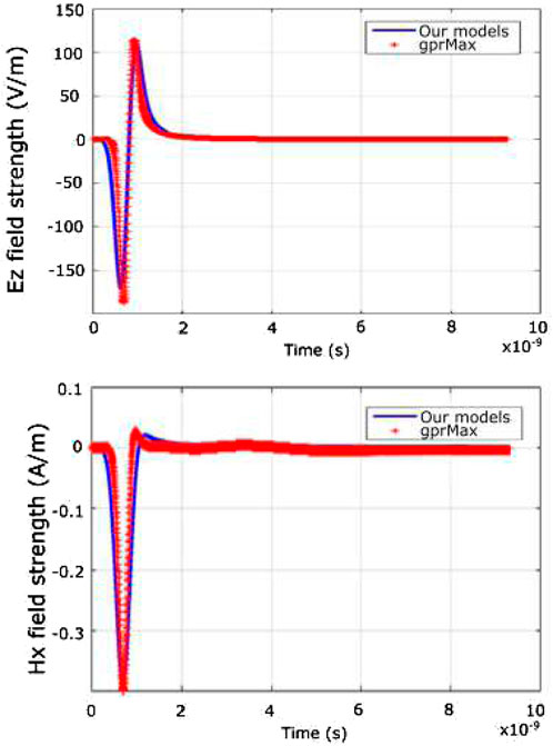
Figure 6. Selected traces of E (top row) and H (bottom row) fields computed for a test model. The responses from our algorithm are shown in blue, and those from gprMax are in red.
4 The magnetic permeability in the transmission and reflection of em waves
In the following numerical experiments, we consider variations in each EM property to analyse the influence of each one of them on the radar signal and its combination for a simultaneous effect. We modelled electric and magnetic components to analyse the effect in both fields.
Since EM field propagation depends on dielectric permittivity, electrical conductivity and magnetic permeability, we expect that each one of these properties affects the radar signal differently, and even though their effects combine into a single EM signal, they can still be individually distinguished. So, to identify their combined effects, we resource to one and two-dimensional models with different physical properties and compute the electric and magnetic fields as they propagate through the media.
To illustrate and explain the differences in reflectivity mechanisms when facing electromagnetic
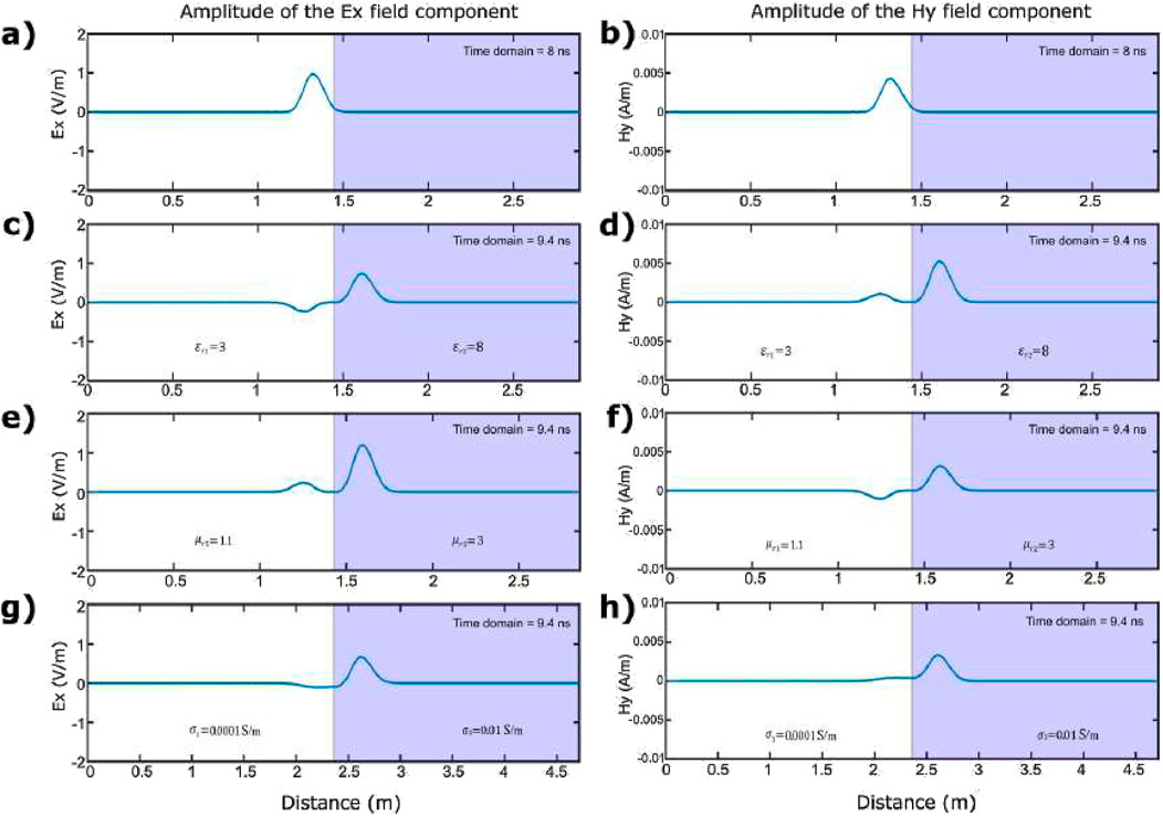
Figure 7. Electric (left) and magnetic (right) fields for two contrasting layers, considering separated variations for
From these 1D experiments, however, we cannot observe any implications related to geometrical divergence. For this, we conducted the two-dimensional experiments of the following sections. In the example from the next section, we explore a 2D EM wave propagation through two media with identical wave speed and attenuation constants, but different
4.1 Testing the need of magnetic permeability in a “coupled-layer model”
Although the theoretical EM framework makes it obvious that signal depends on
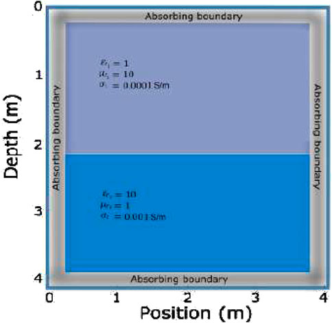
Figure 8. An illustration of the two-dimensional TM-mode array distribution for the coupled layer model. The observation plane lies on the x-y plane.
Following Figure 8, we set
Figure 9 shows the electric and magnetic field traces at an observation point at the surface. In the first row of Figure 9, the magnetic permeability is set equal to
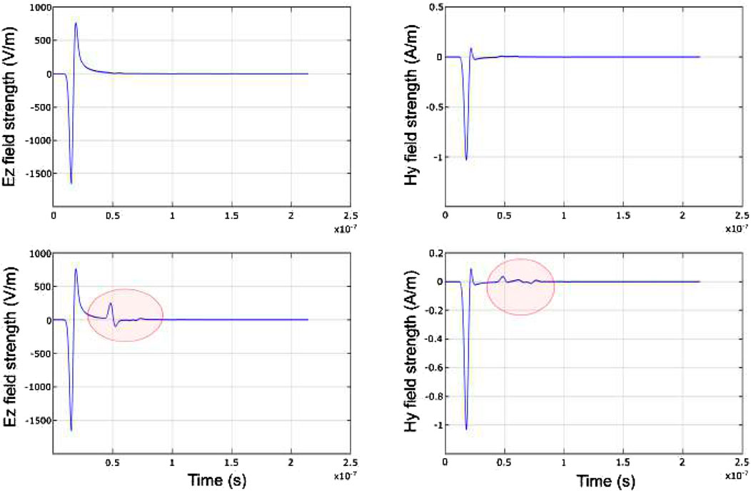
Figure 9. E (left) and H (right) field traces for a model that includes variations in the three properties, designed for the coupled layer model (
The snapshots and shot gathers in Figure 10 show the actual EM wave travelling through the same coupled layer model. Note that the marked reflection would not exist if magnetic permeability was constant, as in the Helmholtz framework (Equation 5). While this example may be difficult to find in nature, it should make evident the need to include magnetic contrast in the numerical modeling of high frequency EM waves, otherwise, the wave propagation would act as if there were only one propagation medium and the signal masks the transition zone.
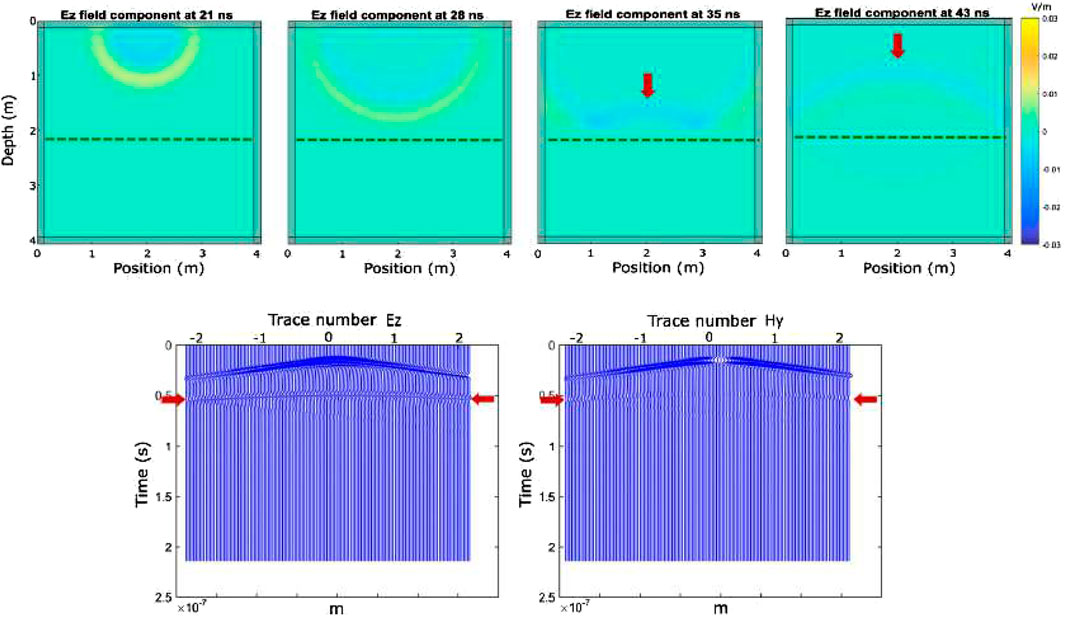
Figure 10. Two-dimensional snapshots (top panels) and radar trace gathers (bottom panels) for the EM wave propagated through the model illustrated in Figure 8. The dotted line in each snapshot indicates the location of the layer boundary; the reflection remarked with red arrows cannot be recovered if
These experiments show the need to consider magnetically heterogeneous media, which is not implemented in most geophysical EM modeling approaches.
4.2 Testing the relevance of magnetic permeability: the Olmec head example
The Olmec heads (Figure 11) are sculptures of members of the nobility of the ancient Olmec culture carved in volcanic stone. These sculptures were found in Quaternary coastal alluvial deposits associated with the currents of the Coatzacoalcos and Uxpana rivers in San Lorenzo Veracruz, Mexico. These
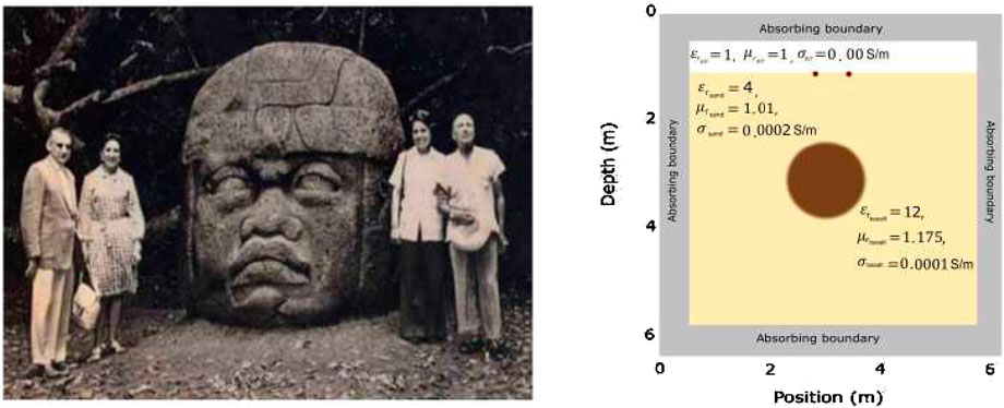
Figure 11. Historic photograph and schematic diagram of the Olmec Head example (left) and our selected model parameters for the Olmec example (right). Image credit Richard Hewitt Stewart/National Geographic Creative, Olmec Colossal Head, Monument 1, San Lorenzo, 1946, in Matthew Stirling, National Geographic, Washington.
Despite their size and allochthonous origin, precise identification of these colossal archaeological remains may still be an interesting target for GPR surveys. Besides natural water moisture alterations, the magnetic permeability of the basalt stone may be the most contrasting feature, and its identification in the signal should lead to the distinction of these volcanic boulders. In this scenario, modeling and identifying the magnetic permeability signal in the GPR data becomes a key element. In Figure 11, we sketch the hypothetical head models and our selected electromagnetic properties.
To illustrate the differences in the actual electric field propagating through the Olmec head, we present some snapshots in Figure 12. Note that after
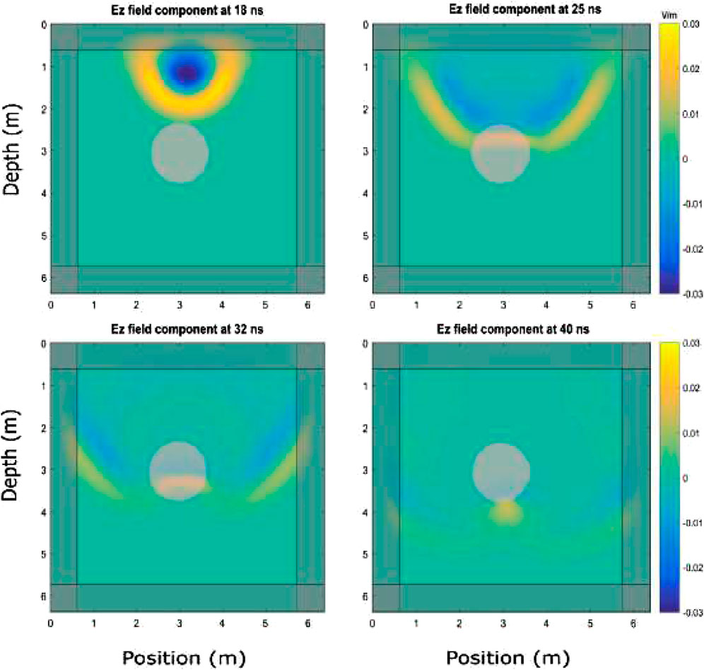
Figure 12. Selected 2D-
To simulate the GPR response of these archaeological remains, we used characteristic properties of the material where the Olmec heads were discovered. The sedimentary rocks of the San Lorenzo area correspond to Miocene and Jurassic deposits of coastal marine origin; they are a sequence of sands and clay sedimented in a marine and shallow-water environment. The rock materials in this area are structured in a layer of compacted coarse-grained sands with clays over finer-grained sands mixed with interspersed clays with high carbon content deposits. The basalt properties selected for the numerical models of Figure 13 are different for
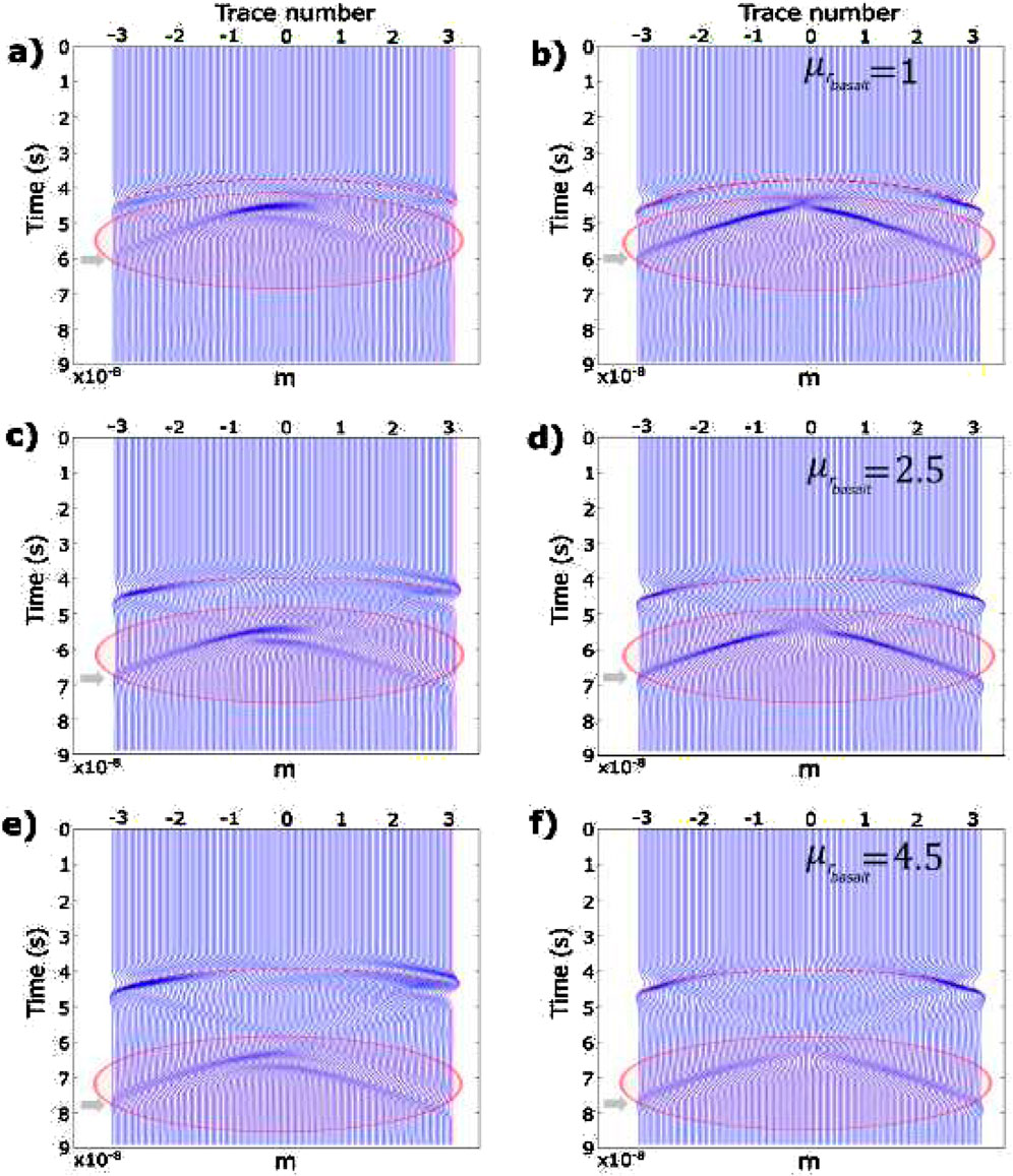
Figure 13. Two-dimensional radargrams for the
Figure 13 shows an example of our computed
We can notice interesting differences in the waveform, amplitude and travel time of the reflected EM wave on the set target. These differences result solely from magnetic permeability variations, confirming the relevance of
In Figure 13, we observe that the first reflected wave increases its amplitude when
To simulate a more realistic scenario for the San Lorenzo examples and explore the complexity added by a conductive layer, we added a hypothetical clay layer above and below the Olmec head. The results (Figure 14) show that the clay layer attenuates the EM signal effectively (see the red blur mark and arrows in the figure); however, the position and thickness of this clay layer may either mask (top panels) or enhance (bottom panels) the target radar response. This effect is especially noticeable for the magnetic field component (right columns).
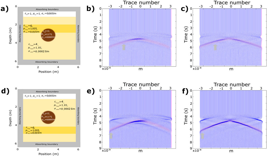
Figure 14. Two-dimensional radargrams for the
In general, we observed that the magnetic permeability contrast notably influences the GPR response, thus facilitating the detection of the target and setting the path for the joint inversion of magnetic and GPR data for any modern archaeological exploration.
5 Conclusion
In this work, a staggered E-H FDTD algorithm for radar modeling was developed by using a coupled Faraday-Ampere framework. The method considers heterogeneities in the three EM properties for radar signal modeling: dielectric permittivity, magnetic permeability and electrical conductivity.
As expected, when the EM wave travels through an homogeneous media, each property affects their transit differently: permittivity determines the wave propagation velocity and electrical conductivity the wave attenuation whereas magnetic permeability influences both aspects. Notably, our results show that the polarity of the reflected vs. transmitted waves are very insightful; a change in
Contrasting values in the magnetic permeability affect not only the transmission/diffusion of the EM wave but also the interactions in the interfaces, resulting in reflected and transmitted waves that cannot be replicated with the sole combination of
Our experiments show how measuring E and H fields allows distinguishing variations from the three properties. Currently, magnetic field components are not considered in radar despite the fact they may contribute to the GPR signal interpretation.
Whereas the combined effect of the radar properties in the GPR signal can make their interpretation challenging, the possibility of use a full three electromagnetic property and both E-H fields propagation for numerical modeling algorithms should lead to a more accurate and discriminative interpretation of the data. Concurrently, the potential acquisition of magnetic field in radar surveys may also contribute to a more unique characterization of the causing heterogeneities.
Given all these possibilities, it is interesting to consider magnetic permeability not only in archaeological examples but also in other applications where magnetic properties may be prominent, such as unexploded ordnances, extraterrestrial explorations, borehole studies and geotechnical studies.
Data availability statement
The data supporting the findings of this study will be made available by the authors upon justified request.
Author contributions
AS: Conceptualization, Formal Analysis, Investigation, Methodology, Software, Visualization, Writing – original draft, Writing – review and editing. LG: Conceptualization, Formal Analysis, Supervision, Validation, Writing – review and editing, Funding acquisition, Methodology.
Funding
The author(s) declare that financial support was received for the research and/or publication of this article. Thanks to SECIHTI for scholarship number 362712, awarded during the doctoral period at CICESE.
Acknowledgments
We thank the Department of Applied Geophysics at CICESE as the hosting institution. We also thank Max Meju for proof-reading the manuscript. We acknowledge the insightful comments made by reviewers, which helped us to improve the quality and clarity of our manuscript.
Conflict of interest
The authors declare that the research was conducted in the absence of any commercial or financial relationships that could be construed as a potential conflict of interest.
Generative AI statement
The author(s) declare that no Generative AI was used in the creation of this manuscript.
Publisher’s note
All claims expressed in this article are solely those of the authors and do not necessarily represent those of their affiliated organizations, or those of the publisher, the editors and the reviewers. Any product that may be evaluated in this article, or claim that may be made by its manufacturer, is not guaranteed or endorsed by the publisher.
Supplementary material
The Supplementary Material for this article can be found online at: https://www.frontiersin.org/articles/10.3389/feart.2025.1632441/full#supplementary-material
References
Aditama, I. F., Syaifullah, K. I., and Saputera, D. H. (2015). “Detecting buried human bodies in graveyard with ground-penetrating radar,” in International workshop and gravity, electrical and magnetic methods and their applications (China: Chenghu), 420–423. doi:10.1190/gem2015-109
Alonso-Díaz, A., Casado-Rabasco, J., Solla, M., and Lagüela, S. (2023). Using InSAR and GPR techniques to detect subsidence: application to the coastal area of “A Xunqueira” (NW Spain). Remote Sens. 15, 3729. doi:10.3390/rs15153729
Berenger, J.-P. (1994). A perfectly matched layer for the absorption of electromagnetic waves. J. Comput. Phys. 114, 185–200. doi:10.1006/jcph.1994.1159
Berezowski, V., Mallett, X., Simyrdanis, K., Kowlessar, J., Bailey, M., and Moffat, I. (2024). Ground penetrating radar and electrical resistivity tomography surveys with a subsequent intrusive investigation in search for the missing Beaumont children in Adelaide, South Australia. Forensic Sci. Int. 357, 111996. doi:10.1016/j.forsciint.2024.111996
Bianco, L., La Manna, M., Russo, V., and Fedi, M. (2024). Magnetic and GPR Data Modelling via Multiscale Methods in San Pietro in Crapolla Abbey, Massa Lubrense (Naples). Archaeol. Prospect. 31, 139–147. doi:10.1002/arp.1936
Breiner, S., and Coe, M. (1972). Magnetic exploration of the olmec civilization: magnetic surveys have been highly successful in locating olmec monuments at the site of the oldest known civilization in mesoamerica. Am. Sci. 60(5), 566–575.
Cabrer, R., Gallardo, L. A., and Flores, C. (2022). Implicit finite-difference time-domain schemes for TDEM modeling in three dimensions. Geophysics 87, E347–E358. doi:10.1190/geo2021-0587.1
Cassidy, N., Eddies, R., and Dods, S. (2011). Void detection beneath reinforced concrete sections: the practical application of ground-penetrating radar and ultrasonic techniques. J. Appl. Geophys. 74, 263–276. doi:10.1016/j.jappgeo.2011.06.003
Cassidy, N. J. (2008). Frequency-dependent attenuation and velocity characteristics of nano-to-micro scale, lossy, magnetite-rich materials. Near Surf. Geophys. 6, 341–354. doi:10.3997/1873-0604.2008023
Conyers, L. B., St Pierre, E. J., Sutton, M.-J., and Walker, C. (2019). Integration of GPR and magnetics to study the interior features and history of Earth mounds, Mapoon, Queensland, Australia. Archaeol. Prospect. 26, 3–12. doi:10.1002/arp.1710
Giannakis, I., Giannopoulos, A., and Warren, C. (2016). A realistic FDTD numerical modeling framework of ground penetrating radar for landmine detection. IEEE J. Sel. Top. Appl. Earth Observations Remote Sens. 9, 37–51. doi:10.1109/JSTARS.2015.2468597
Giannopoulos, A. (2005). Modelling ground-penetrating radar by GprMax. Constr. Build. Mater. 19, 755–762. doi:10.1016/j.conbuildmat.2005.06.007
Hamran, S.-E., Erlingsson, B., Gjessing, Y., and Mo, P. (1998). Estimate of the subglacier dielectric constant of an ice shelf using a ground-penetrating step-frequency radar. IEEE Trans. geoscience remote Sens. 36, 518–525. doi:10.1109/36.662734
Heagy, L. J., and Oldenburg, D. W. (2023). Impacts of magnetic permeability on electromagnetic data collected in settings with steel-cased Wells. Geophys. J. Int. 234, 1092–1110. doi:10.1093/gji/ggad122
Holliger, K., and Bergmann, T. (1998). Accurate and efficient FDTD modeling of ground-penetrating radar antenna radiation. Geophys. Res. Lett. 25, 3883–3886. doi:10.1029/1998GL900049
Klotzsche, A., Jonard, F., Looms, M. C., van der Kruk, J., and Huisman, J. A. (2018). Measuring soil water content with ground penetrating radar: a decade of progress. Vadose Zone J. 17, 1–9. doi:10.2136/vzj2018.03.0052
Komatitsch, D., and Martin, R. (2007). An unsplit convolutional perfectly matched layer improved at grazing incidence for the seismic wave equation. Geophysics 72, SM155–SM167. doi:10.1190/1.2757586
La Bruna, V., Araújo, R., Lopes, J., Silva, L., Medeiros, W., Balsamo, F., et al. (2024). Ground penetrating radar -based investigation of fracture stratigraphy and structural characterization in karstified carbonate rocks, Brazil. J. Struct. Geol. 188, 1. doi:10.1016/j.jsg.2024.105263
Lampe, B., Holliger, K., and Green, A. G. (2003). A finite-difference time-domain simulation tool for ground-penetrating radar antennas. Geophysics 68, 971–987. doi:10.1190/1.1581069
Lazaro-Mancilla, O., and Gómez-Treviño, E. (2000). Ground penetrating radar inversion in 1-D: an approach for the estimation of electrical conductivity, dielectric permittivity and magnetic permeability. J. Appl. Geophys. 43, 199–213. doi:10.1016/S0926-9851(99)00059-2
Molina, C. M., Wisniewski, K. D., Salamanca, A., Saumett, M., Rojas, C., Gómez, H., et al. (2024). Monitoring of simulated clandestine graves of victims using UAVs, GPR, electrical tomography and conductivity over 4-8 years post-burial to aid forensic search investigators in Colombia, South America. Forensic Sci. Int. 355, 111919. doi:10.1016/j.forsciint.2023.111919
Noh, K., Oh, S., Seol, S., Lee, K., and Byun, J. (2016). Analysis of anomalous electrical conductivity and magnetic permeability effects using a frequency domain controlled-source electromagnetic method. Geophys. J. Int. 204, 1550–1564. doi:10.1093/gji/ggv537
Olhoeft, G. (1998). “Electrical, magnetic, and geometric properties that determine ground penetrating radar performance,” in Proceedings of the SeventhInternational conference on ground penetrating radar, 177–182.
Ortega-Ramírez, J., Bano, M., Cordero-Arce, M. T., Villa-Alvarado, L. A., and Fraga, C. C. (2020). Application of non-invasive geophysical methods (GPR and ERT) to locate the ancient foundations of the first cathedral of Puebla, Mexico. A case study. J. Appl. Geophys. 174, 103958. doi:10.1016/j.jappgeo.2020.103958
Palacky, G. J. (2012). Resistivity characteristics of geologic targets. 52–129. doi:10.1190/1.9781560802631.ch3
Pavlov, D. A., and Zhdanov, M. S. (2001). Analysis and interpretation of anomalous conductivity and magnetic permeability effects in time domain electromagnetic data: part I: numerical modeling. J. Appl. Geophys. 46, 217–233. doi:10.1016/S0926-9851(01)00040-4
Persico, R., Negri, S., Soldovieri, F., and Pettinelli, E. (2012). Pseudo 3D imaging of dielectric and magnetic anomalies from GPR data. Int. J. Geophys. 2012, 1–5. doi:10.1155/2012/512789
Pettinelli, E., Burghignoli, P., Pisani, A. R., Ticconi, F., Galli, A., Vannaroni, G., et al. (2007). Electromagnetic propagation of GPR signals in Martian subsurface scenarios including material losses and scattering. IEEE Trans. Geoscience Remote Sens. 45, 1271–1281. doi:10.1109/tgrs.2007.893563
Qiao, S., Zhong, P., Zheng, X., Yi, M., Shu, T., Wang, Q., et al. (2025). Three-dimensional marine magnetotelluric modeling in anisotropic media using finite-element method with coupled perfectly matched layer boundary conditions. J. Phys. Conf. Ser. 3007, 012048. doi:10.1088/1742-6596/3007/1/012048
Reynolds, J. M. (2011). An introduction to applied and environmental geophysics. Hoboken: John Wiley and Sons.
Schultz, J. J., and Martin, M. M. (2012). Monitoring controlled graves representing common burial scenarios with ground penetrating radar. J. Appl. Geophys. 83, 74–89. doi:10.1016/j.jappgeo.2012.05.006
Steven, A., David, F., and Ginger, B. (2010). GPR characterization of a lacustrine UXO site. Geophysics 75, WA221–WA239. doi:10.1190/1.3467782
Van Dam, R. L., Hendrickx, J. M. H., Cassidy, N. J., North, R. E., Dogan, M., and Borchers, B. (2013). Effects of magnetite on high-frequency ground-penetrating radar. Geophysics 78, H1–H11. doi:10.1190/geo2012-0266.1
Virieux, J., and Madariaga, R. (1982). Dynamic faulting studied by a finite difference method. Bull. Seismol. Soc. Am. 72, 345–369. doi:10.1785/bssa0720020345
Warren, C., Giannopoulos, A., and Giannakis, I. (2016). gprMax: open source software to simulate electromagnetic wave propagation for ground penetrating radar. Comput. Phys. Commun. 209, 163–170. doi:10.1016/j.cpc.2016.08.020
Woodward, J., and Burke, M. J. (2007). Applications of ground-penetrating radar to glacial and frozen materials. J. Environ. Eng. Geophys. 12, 69–85. doi:10.2113/jeeg12.1.69
Xiao, T., Xiangyu, H., Cheng, L., Tao, S., Guangjie, W., Bo, Y., et al. (2022). The effects of magnetic susceptibility on controlled-source audio-frequency magnetotellurics. Pure Appl. Geophys. 179, 1–23. doi:10.1007/s00024-022-03050-8
Yee, K. (1966). Numerical solution of initial boundary value problems involving maxwell's equations in isotropic media. IEEE Trans. Antennas Propag. 14, 302–307. doi:10.1109/tap.1966.1138693
Zhou, D., and Zhu, H. (2021). Application of ground penetrating radar in detecting deeply embedded reinforcing bars in pile foundation. Adv. Civ. Eng. 2021, 1–13. doi:10.1155/2021/4813415
Keywords: archaeological geophysics, electromagnetic properties, ground penetrating radar (GPR), magnetic permeability, GPR modeling
Citation: Sánchez AI and Gallardo LA (2025) The magnetic permeability signature in high-frequency electromagnetic data modeling: a case study for GPR approximation. Front. Earth Sci. 13:1632441. doi: 10.3389/feart.2025.1632441
Received: 21 May 2025; Accepted: 22 July 2025;
Published: 20 August 2025.
Edited by:
Xiuyan Ren, Jilin University, ChinaReviewed by:
Arkoprovo Biswas, Banaras Hindu University, IndiaTiaojie Xiao, National University of Defense Technology, China
Copyright © 2025 Sánchez and Gallardo. This is an open-access article distributed under the terms of the Creative Commons Attribution License (CC BY). The use, distribution or reproduction in other forums is permitted, provided the original author(s) and the copyright owner(s) are credited and that the original publication in this journal is cited, in accordance with accepted academic practice. No use, distribution or reproduction is permitted which does not comply with these terms.
*Correspondence: Alejandra I. Sánchez, YWxlamFuZHJhQGNpY2VzZS5lZHUubXg=