UAV aeromagnetic survey of the Acraman impact structure: insights into the central magnetic anomaly

The Acraman Crater in South Australia, a deeply eroded Precambrian impact structure, exhibits a prominent central magnetic anomaly linked to its complex impact history. Previous airborne magnetic surveys captured the broad anomaly but lacked the spatial resolution needed to resolve fine-scale, near-surface features critical for subsurface exploration. To address this, we conducted a high-resolution UAV-based magnetic survey over the crater’s central anomaly, employing a dense 25 m profile spacing and 22.5 m survey altitude. This approach revealed discrete, low-amplitude magnetic features and sharp gradient boundaries, identifying previously undetected localized sources. Data processing included Reduction to the Pole (RTP), Analytic Signal (AS), Vertical Derivative (VD), and Tilt Derivative (TDR) methods to enhance spatial interpretation, while depth estimation using Euler Deconvolution and Radially Averaged Power Spectrum (RAPS) provided source depth constraints. The results indicate a structurally complex magnetic source, extending beyond previously assumed boundaries and containing multiple magnetized bodies. These findings provide critical geophysical insights for future drilling, offering refined targets for sampling impact-modified lithologies that could yield valuable age constraints and insights into the impact process, supporting more accurate subsurface models and guiding future geological investigations.

1 Introduction

The Acraman impact structure, located in South Australia (Figure 1), is one of Earth’s most significant and well-preserved impact sites. Estimated to have formed approximately 580–590 million years ago, this complex crater originally featured a transient cavity ∼40 km in diameter and a final structural rim spanning 85–90 km (Williams and Gostin, 2010; Williams and Wallace, 2003). Its formation was a high-energy event, as evidenced by the presence of shocked minerals, including planar deformation features (PDFs) in quartz, devitrified melt rock, and high-temperature feldspar crystallization, indicating shock pressures exceeding 70 GPa (Timms et al., 2017) and post-shock temperatures above 1,100 °C (Timms et al., 2017; Williams, 1994; Williams and Schmidt, 2021).

Figure 1

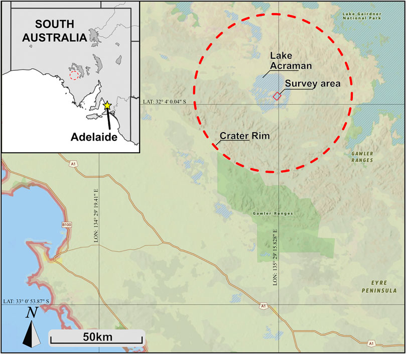
Figure 1. Location of the Acraman crater and the survey site. The background map is sourced from the AGSON Geoscience Portal and is licensed under the Creative Commons Attribution 4.0 International License (CC BY 4.0). ^© Geoscience Working Group (GWG) and Government Geoscience Information Committee (GGIC), 2022.

Previous airborne magnetic surveys, including the PIRSA survey (400 m profile spacing, 80 m altitude) and the GSSA PACE Copper Program survey (200 m profile spacing, 60 m altitude), provided a first order understanding of the crater’s magnetic structure but lacked the resolution necessary to resolve fine-scale, near-surface magnetic features. The broad dipolar anomaly observed in these datasets has been attributed to remanent magnetization in impact-induced melt rocks (Williams et al., 1996), yet its precise distribution, depth, and geological context remain unconstrained. Understanding these characteristics is critical for testing hypotheses regarding the central uplift, impact-generated melt distribution, and potential hydrothermal alteration.

The detailed magnetic characterization of impact structures can be beneficial for understanding their subsurface architecture and identifying optimal sampling locations. Drilling into the central uplift zones of impact craters is widely recognized as a crucial step in impact research, as these zones preserve critical evidence of impact processes and timing (Williams and Schmidt, 2021). The central uplift of Acraman has been identified as a prime candidate for future drilling, with the potential to sample a “hot shock” zone beneath Lake Acraman (Williams and Schmidt, 2021). This could yield impact-reset zircons for precise U-Pb dating, refining the age of the impact event, and facilitating global correlations of Ediacaran biostratigraphy, geochemistry and magnetostratigraphy. However, despite its importance, Acraman remains undrilled, partly due to logistical challenges and the lack of detailed subsurface targeting data. To address this gap, this study presents the highest-resolution magnetic survey of the Acraman central anomaly to date, utilizing a UAV platform. The survey was conducted at an altitude of 22.5 m AGL with a dense profile spacing of 25 m, representing a substantial improvement over previous aeromagnetic dataset. Our study enables precise delineation of anomalies, identification of fine-scale structural variations, and differentiation between near-surface and deep-seated magnetic sources.

Small-UAV magnetometry is now routinely applied to near-surface geophysics (Accomando and Florio, 2024a). Stoll and Moritz (Sto et al., 2013) first demonstrated that a quad-copter-mounted fluxgate can map shallow ferrous infrastructure with metre-scale resolution. The method was soon adapted for defence remediation. Mu et al. (2020) used multirotor data and automated classifiers to locate unexploded ordnance. In mineral exploration, rotary-wing surveys flown at 20–30 m AGL deliver ground-level resolution at substantially lower cost than conventional aeromagnetics, as documented for VMS prospects by Cunningham et al. (2018) and Walter et al. (2020). High density gradiometer grids acquired from lightweight octocopters have also resolved buried archaeological structures without excavation (Accomando and Florio, 2024b). These studies illustrate the established benefits of UAV magnetics-dense sampling, flexible deployment and ease of repeat acquisition in settings where ground or crewed aircraft surveys are impractical. We employ the same approach to investigate the remote, impact modified Acraman structure.

The results of this study refine the spatial and depth constraints of the central magnetic anomaly, providing critical geophysical insights for future drilling feasibility. The findings enhance our understanding of the Acraman impact structure, particularly regarding post-impact thermal evolution, shock-induced remanent magnetization, and structural deformation within the central uplift. Beyond Acraman, this study demonstrates the broader applicability of UAV-based magnetometry for high-resolution geophysical surveys in remote and under-sampled impact structures worldwide.

2 Geological context

The Acraman Crater, located within the Mesoproterozoic Gawler Range Volcanics of South Australia, is a deeply eroded impact structure formed during the Neoproterozoic period. The Gawler Range Volcanics represent a predominantly felsic volcanic suite, formed approximately 1.59 billion years ago through extensive magmatic processes (Blissett, 1987; Fanning et al., 1988; Gostin et al., 1986). The uppermost unit of this suite, the Yardea Dacite, is one of the oldest known felsic volcanic units. It has a current exposed thickness of up to 250 m above the surface, though significant erosion over geological time is believed to have removed up to 6 km of material (Williams and Gostin, 2010).

Lake Acraman, the site of surveyed magnetic anomaly survey, occupies a depression at the center of the crater. The lakebed forms a salt playa, which is predominantly dry but can become waterlogged during periods of heavy rainfall. Its substrate consists of sandy-clayey sediment, with a disjointed salt crust that varies in sturdiness. Surrounding the lake are Quaternary sediments interspersed with outcrops of reddish-brown crystalline rocks. Several elevated features, often referred to as “sandy islands,” rise above the lakebed. These formations are primarily composed of sandy sediments with calcareous intrusions, with localized exposures of crystalline dacite found along the edges and protruding islets (West et al., 2010).

The crystalline dacite outcrops in the area are largely composed of the Yardea Dacite, a high-silica volcanic rock with intermediate chemical properties between andesite and rhyolite (Gostin et al., 1986). These reddish-brown formations are often partially buried under sediment and display evidence of shock metamorphism, such as shatter cones, which are diagnostic of high-pressure impact events. However, the central magnetic anomaly, the primary focus of this study, is located over the flat salt plain area, where no outcrops protrude above the surface.

3 Materials and methods

3.1 UAV and magnetometer

The UAV used for this survey was a commercially available DJI Inspire 2, modified with 3D printed mount to integrate a magnetometer for geophysical measurements (Figure 2). This model was selected for its reliability and advanced features, including redundant key systems, ensuring a high level of safety and multiple camera possibility. It is also equipped with two independent batteries, which allows for efficient battery changes during field operations without interrupting the system or shutting down preplanned flight profiles. This capability allowed for seamless integration of the magnetometer system while maintaining stable flight characteristics essential for high-resolution magnetic surveys (Foss et al., 2025).

Figure 2

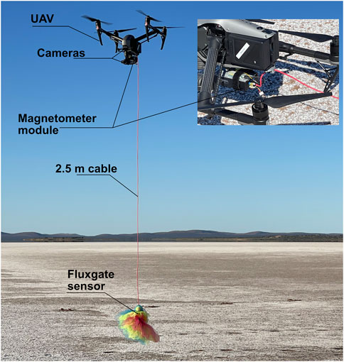
Figure 2. UAV equipped with a magnetometer hovering above the salt plain of Lake Acraman. The magnetometer housing which integrates a GPS receiver, and an independent (3S) battery is rigidly mounted beneath the airframe. The fluxgate sensor is suspended on a cable to minimize magnetic noise. A nylon “skirt” surrounds the sensor, increasing aerodynamic drag to passively damp vibrations and keep the sensor in a stable position throughout the flight.

In addition to the magnetometer, the UAV was equipped with two cameras. One camera (Zenmuse X4S) was able to closely monitor the movement and status of the magnetometer and sensor during flight, while the second camera (Inspire 2 built-in) continuously monitored the terrain in front of the UAV. The video feed was used only for real time monitoring. Survey planning and execution were managed through the Ground Station Pro interface. The flight time of the UAV setup was approximately 20 min, depending on wind intensity. Since the survey area was in a remote location, batteries were recharged using a petrol generator and managed via the TB50 battery station. With seven spare battery kits and a continuous recharging system, the team was able to conduct virtually nonstop flights with only brief landings for battery replacement.

The magnetometer used for mapping purposes was a compact fluxgate magnetometer, developed at the Czech Technical University in Prague specifically for our UAV magnetometry setup with suspended sensor. Compared to a rigidly mounted sensor, a suspended setup at a sufficient distance of sensor beneath the aircraft has the advantage of eliminating electromagnetic interference generated by the UAV (Accomando et al., 2021; Walter et al., 2021). The cable length of 2.5 m was selected based on system integration tests, which showed that at this distance, interference from the UAV is effectively suppressed below the magnetometer’s intrinsic noise level (see Table 1). The sensor employed two dual-axis ring-core fluxgate sensors with dimensions of 26 × 26 × 6 mm and a flat amorphous core design, as described by Petrucha (2016). The complete device underwent scalar calibration using the method described by Merayo et al. (2000), as well as specific vectorial calibration following the procedure outlined by Janosek et al. (2019). The total weight of the suspended magnetometer system, excluding the battery, is approximately 236 g, comprising 85 g for the fluxgate sensor, 31 g for the GPS module, and 120 g for the control electronics. The full specifications of our setup are listed in Table 1.

Table 1

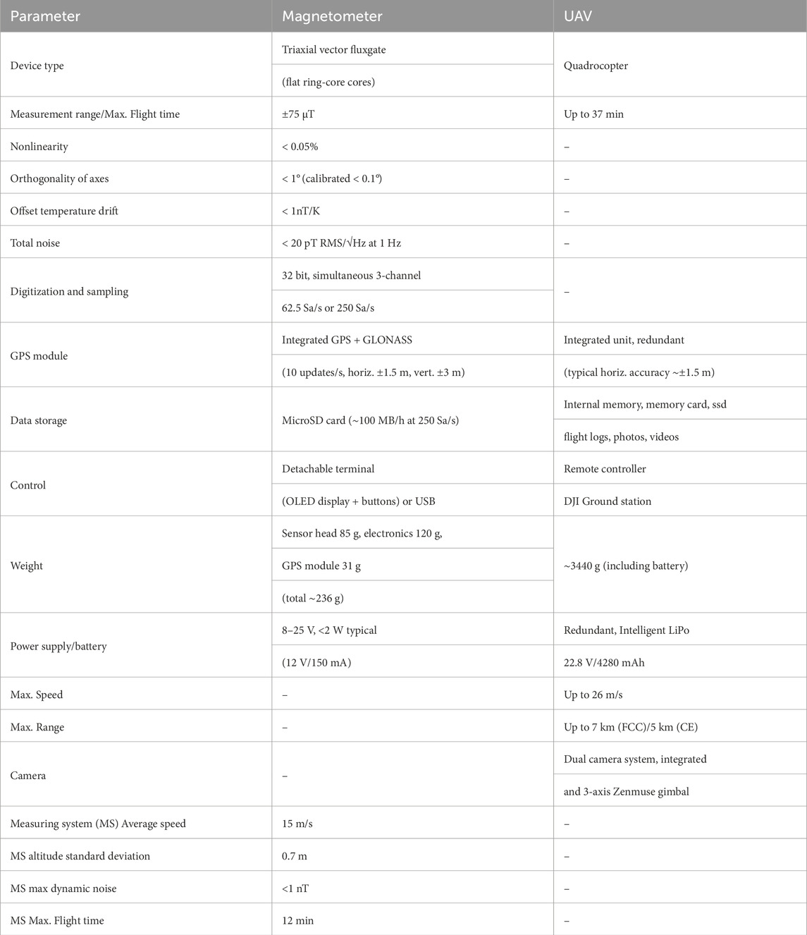
Table 1. Specifications of magnetometer and UAV.

3.2 Survey design

The survey area was selected based on the position of the central magnetic anomaly identified in previous airborne magnetic surveys by Geoscience Australia, which mapped a prominent dipolar anomaly in this region (Figure 3). The entire area lies within a flat salt plain, allowing the UAV to maintain a constant altitude relative to the nominal takeoff level throughout the survey. Vertical accuracy of the UAV is approx. 0.5 m (Table 1). Ground Station Pro was used to control the flight. The UAV was programmed to autonomously follow a grid pattern consisting of profiles 3.5 km in length, spaced 25 m apart, and flown at an altitude of 25 m above the ground (sensor altitude 22.5 m ± 0.5 m). This combination of altitude and line spacing was selected to balance lateral resolution, sensitivity to shallow magnetic sources, and the operational efficiency of the UAV platform. Similar parameters have been successfully applied in previous UAV-based magnetic surveys over geologically complex terrains, (Foss et al., 2025; Parshin et al., 2018; Malehmir et al., 2017; Accomando et al., 2023). The UAV flight paths, shown in Figure 3, illustrate the grid coverage superimposed on earlier 200 m line spacing magnetic maps.

Figure 3

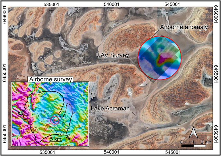
Figure 3. Location of the central magnetic anomaly and spatial distribution of the UAV survey profiles. Airborne survey map is sourced from the AGSON Geoscience Portal and is licensed under the Creative Commons Attribution 4.0 International License (CC BY 4.0). ^© Geoscience Working Group (GWG) and Government Geoscience Information Committee (GGIC), 2022.

To optimize efficiency given the limited battery life of the UAV, flights were planned so that each profile was completed in full before a battery change was required. This ensured that data acquisition was uninterrupted along individual profiles. All flights, excluding landing, were executed autonomously, with the UAV maintaining a direct connection to the base station for real-time monitoring. The operator retained the ability to intervene if necessary. Each flight began at a base station located outside the survey area. Before takeoff, the magnetometer was activated, and data recording was initiated. The UAV ascended vertically to 25 m AGL, moved to the starting point of the profile, and flew along the grid at a constant altitude. At the end of each profile, the UAV turned 90°, moved to the next profile line, and proceeded in the opposite direction. After two consecutive profiles, the UAV returned to the base station for battery replacement. During each battery change, the status of the magnetometer and data recording system was checked to ensure consistent operation. The magnetometer recorded data at a frequency of 62.5 Hz, while the UAV maintained a constant flight speed of ∼14 m/s. For each measurement point, the system recorded three-axis magnetic field data, GPS coordinates, altitude, time, and other sensor parameters. The high-density grid of profiles provided one measured point approximately every 22.4 cm along the flight path and 25 m perpendicular to it. Using this methodology, the survey covered an area of approximately 8 km², with a total profile length of ∼322.72 km. This high-density data acquisition provided detailed spatial coverage of the central magnetic anomaly, enabling the generation of high-resolution maps.

3.3 Data processing

The magnetic data collected during the UAV survey were processed following standard geophysical procedures to ensure data accuracy and reliability (Reeves, 2005). Data points recorded during takeoff, landing, and transitions to the survey grid were excluded to remove measurements outside the survey area. Outliers were identified and removed. Diurnal variation was corrected following Reeves (2005), and heading error was corrected using the directional-averaging method of Hood and Teskey (1989) and Reeves (2005). Since the bias reverses between reciprocal flight lines, correction cancels the offset while preserving geological signal (Pilkington and Keating, 2009). Residual short wavelength line noise (Walter et al., 2019) was then suppressed using standard micro levelling (Minty, 1991) and low-pass filtering (Blakely, 1995). To remove the regional field, the International Geomagnetic Reference Field (IGRF) (Alken et al., 2021) was subtracted from the measured total-field data. The geomagnetic field at the time and location of the survey was approximately 58,000 nT, with an inclination of −64.4° and a declination of 6.2°. By subtracting the measured total magnetic intensity from IGRF data, the residual magnetic intensity (RMI) was calculated. Raw and processed data profiles are shown in Figure 4.

Figure 4

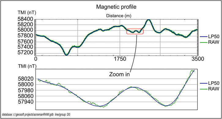
Figure 4. The graph displays a full magnetic profile across the main anomaly. The green line shows the raw TMI data, plotted with increased line weight for visual clarity beneath the processed curve. The blue line represents the data after low-pass filtering. A zoomed inset highlights detailed differences. A cutoff wavelength of 50 m (fiducial based) was used for the low-pass filter, applied in Oasis Montaj. The location of this profile is indicated by the dotted line in Figure 5.

3.3.1 Anomaly maps

To visualize the magnetic data effectively, we calculated and applied several data enhancement techniques on top of standard RMI anomaly map. These techniques aimed to amplify specific magnetization representations while reducing unwanted features. Data processing was performed using Geosoft Montaj with MAGMAP extension. Data were gridded using minimum curvature with 10 m cell size. Key processing techniques included reduction to pole (RTP) which was applied on RMI data, analytic signal (AS), vertical derivative (VD) and tilt derivative (TDR) were used on RTP RMI.

Reduction to the Pole (Figures 5 and 6A) was applied to correct for the effects of the Earth’s magnetic field inclination and declination, relocating anomalies over their sources to support geological interpretation (Reeves, 2005; Baranov and Naudy, 1964; Pereira et al., 2021). At the Acraman structure, where the geomagnetic inclination is moderate (−64.4°), RTP provides limited but noticeable improvement in anomaly positioning. However, because RTP assumes purely induced magnetization aligned with the present-day field, its effectivity can be affected in the presence of strong remanent magnetization (Baranov and Naudy, 1964). Given the impact-related nature of Acraman, we interpreted RTP maps with caution.

Figure 5

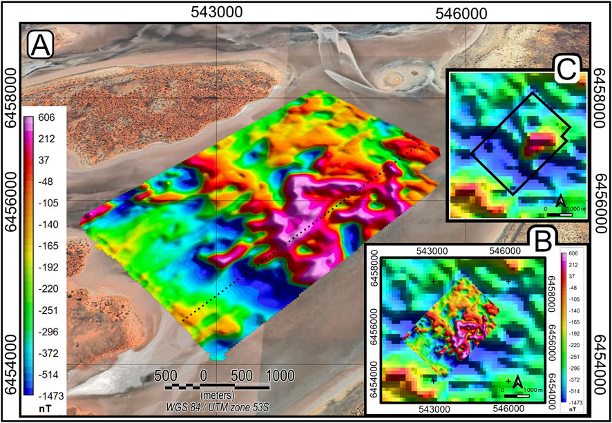
Figure 5. (A) UAV-based Residual Magnetic Intensity (RMI) map of the central magnetic anomaly over the salt basin of Lake Acraman. The dotted line indicates the magnetic profile shown in Figure 4. (B) Overlay with the previous PIRSA airborne survey illustrates the significantly enhanced resolution achieved through the lower flight altitude (22.5 m AGL) and tighter profile spacing (25 m), compared to the PIRSA survey’s 80 m AGL and 400 m profile spacing. The improved resolution provides a more detailed delineation of the anomaly’s structure, allowing for better spatial characterization of magnetic sources. (C) position of UAV survey over airborne map. Airborne survey map is sourced from the AGSON Geoscience Portal and is licensed under the Creative Commons Attribution 4.0 International License (CC BY 4.0). ^© Geoscience Working Group (GWG) and Government Geoscience Information Committee (GGIC), 2022.

Figure 6

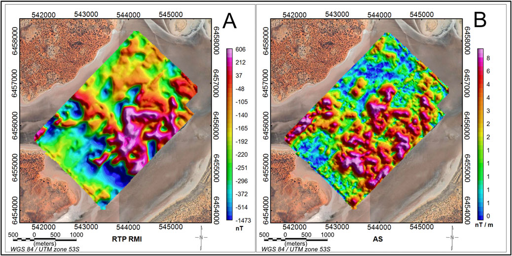
Figure 6. (A) Reduced to Pole RMI showing the spatial distribution of magnetic anomalies corrected for skewness, aligning them directly above their causative sources within the central Acraman anomaly. (B) Analytic signal highlighting the edges and shallow magnetized bodies, independent of magnetization direction.

Analytic Signal (Figure 6B) was applied to aid the interpretation of magnetic anomalies by incorporating both horizontal and vertical gradients of the magnetic field, offering an amplitude-based visualization of the total gradient (Salem et al., 2008). This method is particularly valuable for lithological interpretation, as it produces amplitude maxima over magnetized bodies, with reduced sensitivity to the direction of magnetization (Roest et al., 1992). While AS is generally less affected by remanent magnetization than total magnetic intensity, it is not entirely immune to its influence (Agarwal and Shaw, 1996).

The transformation was computed in the frequency domain, which allows efficient gradient estimation but does not inherently distinguish between shallow and deep sources (Blakely, 1995). In the context of the Acraman impact structure, where remanent magnetization associated with melt-bearing rocks is known to affect the central anomaly (Williams et al., 1996; Schmidt and Williams, 1991), AS was helpful in outlining the extent of magnetized bodies despite the presence of remanence. However, interpretations were made with caution, acknowledging the method’s limitations in the presence of complex magnetization patterns.

Vertical Derivative (Figure 7A) was applied to emphasize short-wavelength components of the magnetic field by enhancing shallow features and suppressing regional trends (Blakely, 1995). As a high-pass filter, VD highlights sharp contacts, faults, and near-surface intrusions but may amplify noise, particularly in datasets with uneven sampling or low signal-to-noise ratio (Pilkington and Keating, 2009). Given these limitations, we applied only the first-order vertical derivative to enhance near-surface features while minimizing noise amplification. Higher order derivatives were not applied, as they offered no additional structural detail and introduced significant noise. The first order VD shows only minor high frequency streaks, primarily at the ends of survey lines. These artefacts result from complex, non-periodic sensor motion during UAV deceleration, producing transient signal components with wavelengths that lie within the passband of the applied 50 m low-pass filter, as noted in the caption of Figure 7. Tilt Derivative (Figure 7B) was applied to enhance subtle magnetic variations by emphasizing local gradients and edges in the magnetic field, supporting the identification of possible structural features within the surveyed area (Salem et al., 2008; Miller and Singh, 1994) (Miller and Singh, 1994; Salem et al., 2008). Within the surveyed area of the Acraman structure, TDR aided in highlighting localized structural patterns and magnetic gradients associated with near-surface deformation features. TDR normalizes the vertical and horizontal gradients of the magnetic field, enhancing both shallow and deeper features but limiting the ability to distinguish between them due to amplitude equalization (Pereira et al., 2021). As TDR is derived from the same first order VD grid, it inherits the same noise floor; artefacts are again restricted to the profile ends, leaving the interior of the map unaffected. Since TDR was applied to RTP data, it retains sensitivity to magnetization direction.

Figure 7

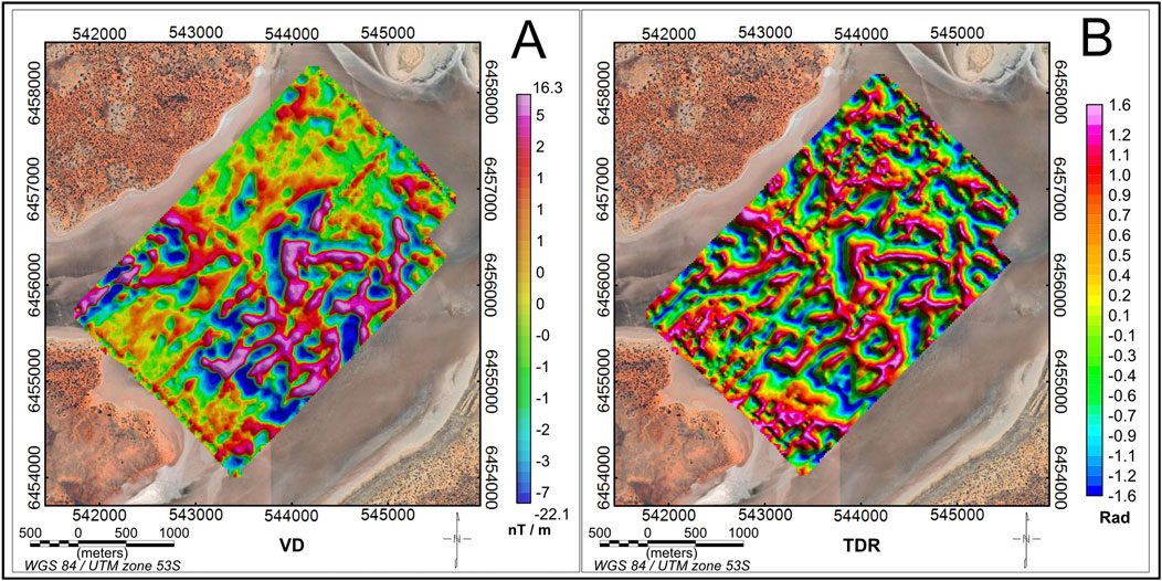
Figure 7. (A) Vertical Derivative (VD) map of the central Acraman anomaly, enhancing short-wavelength magnetic features and shallow sources. Positive VD values, indicating regions where the magnetic field strength increases with depth, often corresponding to the tops or edges of shallow magnetized bodies. Negative VD values, marking transitions where the magnetic field decreases with depth, typically associated with the edges or downward slopes of magnetic anomalies. Intermediate values indicate regions with minimal vertical change in magnetic intensity, suggesting deeper or more homogeneous magnetic sources. (B) Tilt Derivative (TDR) map highlighting the edges, extents, and depth variations of magnetic sources. TDR values are in radians, ranging from −1.6 (blue) to 1.6 (pink). Values near ±π/2 (≈±1.57 radians) correspond to strong magnetic field gradients, typically marking the edges of magnetized bodies. Zero values (≈0 radians) indicate the precise boundaries of magnetic sources. Gradual transitions in TDR values represent smoother magnetization variations, which may correlate with gradual lithological changes or deeper magnetic sources. At the ends of some survey lines, the VD and TDR grids show short, high-frequency artefacts caused by complex motion of the suspended sensor as the UAV decelerated prior to turning. These transient signals were not fully suppressed by the applied 50 m low-pass filter. Derivative operators accentuate these localised steps, causing them to appear as streaks at profile ends. Eliminating them would require trimming data or applying a shorter filter cutoff-both of which would unnecessarily reduce resolution elsewhere. Data collected during turns were removed during preprocessing; the minor artefacts that remain are confined to the grid margins and do not affect interpretation of the main anomaly.

3.3.2 Depth estimates

The Magnetic source depths were estimated using two complementary methods: Euler Deconvolution and Radially Averaged Power Spectrum analysis.

Euler Deconvolution was applied to estimate the depth to the top of magnetic sources using the RTP RMI grid and computed magnetic gradients. The analysis was performed in VOXI Earth Modelling with a 10 × 10 cell window size, following the method of Thompson (1982). Two structural index (SI) values were tested: SI = 1 for elongated sources such as fractures or dike-like features, and SI = 2 to explore more compact geometries. A tolerance of 15% was used, referring to the acceptable error in depth estimation relative to the modeled source position.

Depth estimates for both SI values were visualized in 2D for comparison (Figure 8), while SI = 1 results were interpolated into a 3D surface with 10× vertical exaggeration to aid visual interpretation (Figure 9). This surface was overlaid with the RTP RMI grid, enabling direct comparison between depth structure and the observed magnetic anomaly pattern (Pilkington and Keating, 2009).

Figure 8

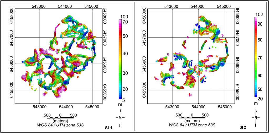
Figure 8. Euler deconvolution depth solutions for the central Acraman magnetic anomaly. The SI 1 (left) shows a broader set of solutions with shallowest results close to 5 m, while the SI 2 solutions (right) show depths from 20 m. Color coding represents estimated depths, with red, pink indicating deeper sources and colors blue shallower sources. The clustering of shallow solutions near strong magnetic gradients suggests near-surface magnetic bodies, while deeper solutions align with the broader anomaly structure, indicating deeper-seated magnetic sources.

Figure 9

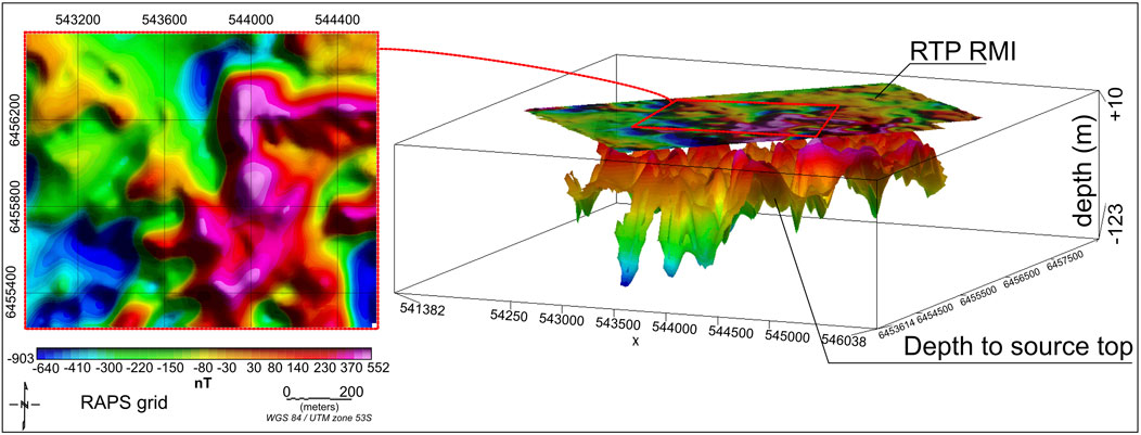
Figure 9. 3D depth model of the magnetization basement based on Euler deconvolution depth solutions (right). The lower surface represents the estimated depth to the top of magnetic sources. Color coding corresponds to depth, with red indicating shallower magnetic sources and green, blue representing deeper structures. The upper grid is +10 m offset and displays the RTP RMI map, providing a direct comparison between surface magnetic anomalies and their inferred subsurface sources. This model highlights the depth variations and complexity of the magnetic structure within the central Acraman anomaly. Area of the survey where RAPS analysis was performed is shown on the left.

Radially Averaged Power Spectrum analysis was used to estimate average source depths from the magnetic field’s power spectrum. This method is particularly well-suited for UAV surveys, offering a noise-resistant, frequency-domain approach to depth estimation by analyzing the decay of spectral energy with increasing wavenumber (Maus and Dimri, 1996; Spector and Grant, 1970). The slope of linear segments in the log-power vs. frequency plot provides an estimate of the average depth to the top of magnetic sources (Pereira et al., 2021; Rebolledo-Vieyra et al., 2010).

This spectral approach complements Euler Deconvolution by providing an independent depth estimation method, allowing for comparison and cross-validation of results. By analyzing depth estimates derived from frequency-domain techniques, RAPS helps assess the consistency and reliability of the Euler-derived depths and provides additional confidence in the interpretation of subsurface structures in the Acraman Crater’s central anomaly.

4 Results

This UAV magnetic survey of the Acraman Crater generated high-resolution data that significantly enhanced the spatial definition of the central magnetic anomaly. Compared to previous aeromagnetic datasets (PIRSA, GSSA) (Figure 3), the improved magnetic maps provide a more detailed visualization of fine-scale magnetic variations, including isolated magnetic highs and localized structural features that were not clearly resolved in earlier surveys (Figure 5). The low-altitude data acquisition also supports more precise depth estimates for shallow magnetic sources within the surveyed area. Together, these advancements offer detailed insights into the distribution of magnetic sources, supporting the identification of potential drilling targets where localized magnetic anomalies suggest denser or more magnetized material.

The following sections present the results obtained from individual processing and interpretation techniques, including RTP, AS, VD, TDR, Euler Deconvolution, and RAPS depth analysis.

4.1 Enhanced magnetic maps

The residual magnetic intensity (RMI) map generated from the UAV data provides a comprehensive view of the central magnetic anomaly. Based on previous surveys, the anomaly was characterized by a dipolar feature with a distinct high and low magnetic intensity zone. However, the UAV data reveal complex shape and additional small-scale variations and edges within the anomaly that were unresolved in earlier datasets. An overlay with the lower-resolution RMI map from previous aeromagnetic surveys (Figure 5B) demonstrates the improved detail provided by the UAV survey.

The Reduction to the Pole (RTP) transformation ideally correct data for the effects of geomagnetic inclination and declination. However, the effect of this transformation is relatively minor in our dataset (Figure 6A), partially due to the moderate local geomagnetic inclination (−64.4° at Acraman), which naturally produces more vertically oriented anomalies, and the influence of remanent magnetization, which RTP is not designed to correct (Baranov and Naudy, 1964; Ugalde et al., 2007). In the survey region, many anomalies remain asymmetrical or dipolar even after RTP, suggesting the presence of remanent magnetization or inclined source geometries. This interpretation is further supported by the Analytic Signal map (Figure 6B), where several anomalies that are dipolar or asymmetrical in RTP appear as symmetrical, high-amplitude features, consistent with remanent effects or complex source geometries. Additionally, regions that appear as negative anomalies on the TMI map often correspond to positive features on the AS map, a characteristic that can indicate remanent magnetization with a direction opposite to the present geomagnetic field (Blakely, 1995; Reid, 1980).

Figure 7 presents the Vertical Derivative and Tilt Derivative maps, which provide further insights into the structure and distribution of magnetic anomalies within the surveyed area. The Vertical Derivative map (Figure 7A) emphasizes shallow magnetic sources by enhancing short-wavelength components, effectively delineating sharp boundaries and near-surface anomalies. These high-gradient zones are concentrated in regions with the strongest RMI amplitudes. The closely spaced positive and negative gradients in these areas indicate rapid lateral changes in magnetic properties, consistent with highly disrupted and multi-directionally magnetized materials likely reflecting remnant of intense fracturing, shock brecciation, and localized melt rock formation in the impact-modified zone.

The Tilt Derivative map (Figure 7B) reveals a more chaotic distribution of magnetic gradients, capturing both shallow and deeper structures that are less pronounced in the Vertical Derivative map. Unlike VD, which primarily attenuates deeper signals and amplifies near-surface sources, TDR normalizes amplitude variations, making it sensitive to a broader range of sources. In our case, this results in a complex, irregular pattern without clear systematic alignment, consistent with the extensive fracturing and disruption expected in the central uplift. Elongated anomalies are present and are consistent with large positive and negative areas in RMI, but the overall distribution is disordered, likely reflecting the intense deformation and multi-phase remanent magnetization associated with the Acraman impact event.

4.2 Depth estimates

Euler Deconvolution yielded depth solutions for both structural indexes SI = 1 and SI = 2, providing insights into the depth distribution of magnetized sources (Figure 8). The depth values represent the estimated position of the upper edge of the magnetic body. For SI = 1, depths ranged from 3.5 m to 100 m, with a mean depth of 38 m. For SI = 2, the range toward deeper values (20–102 m) with a mean depth of 70 m, indicating a potential shift towards detecting deeper structures. SI = 1 returned approximately twice as many valid solutions consistent with a greater number of shallow features being captured under this assumption compared to SI = 2.

Following standard procedure in Oasis Montaj, Euler solutions were retained only when algebraic misfit was ≤15%, which constrains the formal 95% confidence interval of each solution to ±0.15H (Pilkington and Keating, 2009; Thompson, 1982). For the mean depths retrieved here, this equates to ±6 m for SI = 1 and ±10 m for SI = 2. These values represent the expected individual error bounds, and are consistent with the resolution expected from a 10 × 10-cell window over 10 m data grid.

The spatial distribution of depths also differs by structural index. SI = 1 emphasizes a dense array of shallow anomalies between 10 and 30 m across much of the survey area. SI = 2 highlights more clustered, deeper anomalies. In both cases, coherent depth gradients and localized clusters suggest the presence of vertically zoned source bodies.

2D plots (Figure 8) illustrate the variations in solution distribution and depth between the two SI values, while a 3D visualization with 5× vertical exaggeration provides enhanced spatial context (Figure 9). The 3D surface of top of magnetic source was gridded from inverted 3D Euler solutions for SI1 and was overlaid with the RTP RMI plot, allowing direct correlation between the magnetic anomaly and subsurface structure. These results refine the understanding of the Acraman Crater’s central magnetic anomaly by offering multiple depth models based on different structural assumptions.

The RAPS analysis (Figure 10) identified magnetic source up to depths ∼90 m. These results closely align with the depth estimates derived from Euler Deconvolution, which also indicate major magnetic sources within the 30–100 m range. RAPS was calculated for regirded area of RTP RMI as shown in Figure 9. Three linear segments in and yield slopes of −1.142 ± 0.068 rad (−65.4° ± 3.9°), −0.672 ± 0.057 rad (−38.5° ± 3.3°), and −0.332 ± 0.034 rad (−19.0° ± 2.0°), corresponding to mean depths of 26 ± 3 m, 54 ± 5 m, and 91 ± 6 m, respectively (95% confidence). These values follow standard spectral depth interpretation (Spector and Grant, 1970).

Figure 10

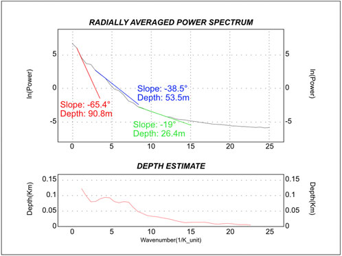
Figure 10. Radially Averaged Power Spectrum and depth estimates for the prominent anomaly shown in Figure 9. The depth estimate curve was derived from spectral analysis during the RAPS computation. Three additional slopes, corresponding to deep (red), intermediate (blue), and shallow (green) sources, were calculated based on the slope of the power spectrum, providing an independent estimate of magnetic source depths.

5 Discussion

Previous airborne magnetic surveys over the Acraman Crater delineated the central magnetic anomaly, however, their resolution was constrained by flight altitude and profile spacing limitations. Standard aeromagnetic surveys, such as the PIRSA and the GSSA survey under the PACE Copper Program were optimized for regional scale mapping but lacked the spatial resolution necessary to resolve finer-scale, near-surface magnetic variations. The technical and financial constraints of airborne surveys necessitate higher flight altitudes and broader line spacing, limiting their ability to detect small-scale variations in magnetic anomalies.

In contrast, our UAV-based magnetic survey represents advancement in resolution and spatial detail increasing data density, enhancing the detectability of isolated and shallow magnetic sources as shown in Figure 5. This allows for a better spatial characterization of the investigated part of central uplift and associated magnetic anomalies. Enhanced spatial resolution not only refines our understanding of the internal structure of the central anomaly but also provides a more precise geophysical framework for identifying potential drilling and sampling locations. This is particularly useful given the potential for recovering impact-reset zircons for precise U-Pb dating, as suggested by and Schmidt (2021). A comparison between the UAV derived total magnetic intensity map and prior datasets highlights the improved resolution and ability to capture fine scale variations (Figure 5B). The central anomaly, previously thought to be a simple dipolar feature (Williams et al., 1996), exhibits complex internal structure, suggesting a heterogeneous distribution of magnetized bodies. The more pronounced positive cluster is extended in the north-south direction and reaches an amplitude of up to 600 nT. The negative (up to −1,400 nT) lobe is located to the south and extends northwest to southeast. Extending the survey area further east would likely provide additional insights into this feature.

5.1 Magnetic data processing and interpretation

The (Figure 6A) shows many anomalies remain asymmetrical or dipolar after the RTP transformation, suggesting the presence of remanent magnetization or dip of the source bodies. This is consistent with findings that impact melt and highly shocked lithologies can retain multi-directional remanent magnetization not fully corrected by RTP alone (Pohl et al., 1988; Pilkington and Grieve, 1992).

The AS map (Figure 6B) enhances the detection of magnetized bodies irrespective of polarity, revealing multiple, spatially distinct magnetized regions. Notably, anomalies that appear dipolar or asymmetrical in the RTP map manifest as symmetrical, high amplitude features in the AS map, indicating remanent effects or complex source geometries. Furthermore, regions that are negative in the TMI or RMI maps often correspond to strong positive anomalies in the AS map, reflecting remanently magnetized sources with magnetization directions differing significantly from the present-day geomagnetic field (Blakely, 1995; Reid, 1980).

The VD map (Figure 7A) emphasizes short-wavelength features, delineating sharp lateral boundaries of shallow magnetic sources. These high-gradient zones likely correspond to regions of intense fracturing and localized brecciation, consistent with mechanical disruption in the central uplift. The correlation between high VD gradients and AS intensity peaks reinforces the interpretation of near-surface magnetized material. Depth estimates from Euler deconvolution and Radially Averaged Power Spectrum analyses indicate that many of these features are shallow, with sources at depths of 10–30 m (Figures 8, 9), supporting the presence of shock-fractured basement or fragmented impact melt (Williams et al., 1996).

The TDR map (Figure 7B) captures a more chaotic distribution of magnetic gradients, including deeper structures not fully resolved in the VD map. This complexity reflects the multi-phase and heterogeneous nature of the central uplift, where intense deformation and variable remanent magnetization produce intricate magnetic signatures (Pilkington and Grieve, 1992; Grieve et al., 1991). The lack of systematic alignment in the TDR map likely results from impact-induced brecciation and fracture networks, leading to disordered, multi-scale magnetic sources.

5.2 Geological context and depth estimates

The Acraman impact event significantly altered the pre-existing volcanic lithology, producing a complex central magnetic anomaly. Similar features in other large impact structures, such as Sudbury (Pilkington and Grieve, 1992), Manicouagan (Eitel et al., 2016), and Chicxulub (Rebolledo-Vieyra et al., 2010), have been attributed to the remanent magnetization of impact melt sheets and highly shocked basement lithologies. These structures often exhibit multi-phase remanent magnetization, reflecting intense fracturing, localized melting, and variable cooling of impact-modified rocks.

Outcrop measurements within the Acraman structure display an order-of-magnitude variation in magnetic susceptibility (χ) (Williams et al., 1996). Although χ records only the induced component of magnetisation (Dunlop and Özdemir, 1997), such pronounced lateral variability indicates sharp contrasts in magnetic-mineral assemblage created by patchy melting, shock heating and post-impact hydrothermal alteration. Laboratory and field studies have shown that where magnetic mineralogy is heterogeneous, equally heterogeneous remanent components (TRM/CRM) are commonly generated (Pilkington and Grieve, 1992; Henkel and Reimold, 1998). Thus the observed χ variation is not a direct measure of remanence, but it is fully consistent with a lithological framework in which spatially variable remanent magnetisation can develop within the central uplift.

Depth estimates from Euler deconvolution (Figure 8) and Radially Averaged Power Spectrum analyses (Figure 10) provide additional context for the vertical (depth) distribution of magnetic sources within the central uplift. The Euler analysis identified shallow magnetized sources at depths ranging from 5 to 100 m, with SI1 highlighting shallow features (5–30 m) and SI2 capturing deeper structures (20–100 m). The RAPS analysis supports this interpretation, revealing multi-layered magnetic sources with well-defined depth distributions, including shallow (∼26 m), intermediate (∼53 m), and deep (∼90 m) components. It is important to note that in Oasis montaj, the window size used in Euler deconvolution (10 × 10) directly influences the maximum depth of solutions. A larger window size allows for the detection of deeper sources, while a smaller window size is more sensitive to shallow features. Therefore, the maximum depth estimates obtained are inherently limited by the chosen window size during analysis.

This multi-layered structure suggests that the central uplift contains a heterogeneous assemblage of fragmented, variably magnetized blocks, consistent with the intense mechanical disruption and variable cooling rates expected in impact-modified terranes. The observed correlation between shallow sources and high AS intensities further supports this interpretation, as these regions likely host shock-fractured basement or fragmented melt rocks.

5.3 Implications for impact cratering and future work

UAV magnetometry has proven to be valuable tool for refining the geological and geophysical understanding of impact structures. The complex magnetic pattern observed within the Acraman central anomaly suggests a history of shock metamorphism, partial melting, and possible hydrothermal alteration, which are common in large impact structures (Williams and Schmidt, 2021; Gilder et al., 2018). Previous studies have noted that deeply eroded impact structures often retain magnetic signatures that provide insights into subsurface processes (Rebolledo-Vieyra et al., 2010; Eitel et al., 2016). The elliptical magnetic low and high-amplitude dipolar anomaly identified in previous aeromagnetic data (Williams and Gostin, 2010) align well with the UAV-derived results, confirming that remanent magnetization is a key factor influencing the observed anomalies.

One of the most significant implications of these findings is the potential for targeted future drilling in the central uplift region. Previous studies have proposed that deep drilling into the ‘hot shock’ zone could recover zircons with U–Pb ratios reset by the impact, providing a more precise age for the event (Williams and Schmidt, 2021). The UAV survey results, which delineate the spatial distribution of the magnetic anomaly offer valuable guidance for selecting optimal drilling locations. The present 8 km² UAV grid was intentionally centred on the strongest magnetic high of the Acraman central uplift, providing the resolution needed to refine this key anomaly while acknowledging that it captures only a small portion of the 85–90 km structure. To place these results in a crater-wide context, future work could include radial UAV transects that link the central grid to the annular ring fault, together with targeted palaeomagnetic and rock sampling to constrain magnetization directions. A multidisciplinary extension incorporating high resolution Bouguer gravity, shallow seismic imaging, or near surface EM soundings would further reduce model non-uniqueness. Bruno et al. (2024) demonstrated that such integrated datasets can significantly improve structural interpretations in complex tectonic settings. Applying a similar strategy at Acraman could therefore enhance both depth control and lithological discrimination across the entire crater.

5.4 Survey effectiveness

In addition to its scientific advantages, the UAV-based survey offers a highly cost-effective alternative to traditional airborne or handheld magnetometry. The survey covered an area of 8 km², with a total of 322 km of profiles. The UAV operated using two batteries simultaneously, requiring 50 battery pair replacements throughout the survey. To maintain continuous measurements, we used 12 batteries (6 pairs) in rotation, ensuring uninterrupted operation by constantly recharging in cycles. The total operational battery cost for this survey was approximately $90 (considering price of the battery and cycle lifespan). Recharging consumed 1 kW over 24 h. These practical considerations highlight the established advantages of UAV magnetometry in remote or logistically challenging terrains, such as the Acraman Crater. While these benefits are well documented in the literature (Cunningham et al., 2018; Walter et al., 2020; Archer, 2023), our results further demonstrate how UAV systems can enable dense spatial sampling, flexible deployment, and the potential for repeat surveys in previously inaccessible environments.

6 Conclusion

This study provides the highest-resolution magnetic survey of the Acraman impact structure’s central anomaly to date, surpassing previous airborne datasets in spatial detail and data density. Using UAV-based magnetometry with a 25 m profile spacing and 22.5 m flight altitude, we mapped fine-scale magnetic variations that were previously undetected, revealing a structurally complex anomaly composed of multiple magnetized sources rather than a simple dipolar feature.

These sources are likely associated with impact-modified lithologies, uplifted volcanic rocks, and possible remanent magnetization effects. The refined mapping of these features provides crucial guidance for future drilling in the central uplift zone, where impact-modified lithologies could host impact-reset zircons for improved age constraints refining the age of the impact event, and facilitating global correlations of Ediacaran biostratigraphy, geochemistry, and magnetostratigraphy.

Our results highlight the advantages of UAV-based magnetometry for impact crater research, offering cost-effective, high-resolution data acquisition that is logistically adaptable to remote environments. Future work should expand the surveyed area and integrate additional geological data from drilling samples to further refine subsurface models.

Data availability statement

The data presented in this study are available in public repository 10.6084/m9.figshare.29045021.

Author contributions

MT: Data curation, Formal Analysis, Funding acquisition, Investigation, Project administration, Resources, Software, Visualization, Writing – original draft. GK: Funding acquisition, Investigation, Methodology, Resources, Supervision, Validation, Writing – review and editing. VP: Resources, Writing – review and editing.

Funding

The author(s) declare that financial support was received for the research and/or publication of this article. This research was supported by the Czech Science Foundation Grant [23-06075S], Ministry of Education, Youth and Sports of the Czech Republic (Project No. LUAUS25082) and Center for Geosphere Dynamics (UNCE SCI/006).

Acknowledgments

The authors thank Dr. Clive Foss for support with survey organization and Darja Kawasumi for logistical support.

Conflict of interest

The authors declare that the research was conducted in the absence of any commercial or financial relationships that could be construed as a potential conflict of interest.

Generative AI statement

The author(s) declare that no Generative AI was used in the creation of this manuscript.

Any alternative text (alt text) provided alongside figures in this article has been generated by Frontiers with the support of artificial intelligence and reasonable efforts have been made to ensure accuracy, including review by the authors wherever possible. If you identify any issues, please contact us.

Publisher’s note

All claims expressed in this article are solely those of the authors and do not necessarily represent those of their affiliated organizations, or those of the publisher, the editors and the reviewers. Any product that may be evaluated in this article, or claim that may be made by its manufacturer, is not guaranteed or endorsed by the publisher.

Abbreviations

RMI, Residual Magnetic Intensity; TMI, Total Magnetic Intensity; VD, Vertical Derivative; TDR, Tilt Derivative; AS, Analytic Signal; RAPS, Radially Averaged Power Spectrum; RTP, Reduction to the Pole; PIRSA, Primary Industries and Regions SA.

References

Accomando, F., and Florio, G. (2024a). Applicability of small and low-cost magnetic sensors to geophysical exploration. Sensors 24, 7047. doi:10.3390/s24217047

PubMed Abstract | CrossRef Full Text | Google Scholar

Accomando, F., and Florio, G. (2024b). Drone-borne magnetic gradiometry in archaeological applications. Sensors 24, 4270. doi:10.3390/s24134270

PubMed Abstract | CrossRef Full Text | Google Scholar

Accomando, F., Vitale, A., Bonfante, A., Buonanno, M., and Florio, G. (2021). Performance of two different flight configurations for drone-borne magnetic data. Sensors 21, 5736. doi:10.3390/s21175736

PubMed Abstract | CrossRef Full Text | Google Scholar

Accomando, F., Bonfante, A., Buonanno, M., Natale, J., Vitale, S., and Florio, G. (2023). The drone-borne magnetic survey as the optimal strategy for high-resolution investigations in presence of extremely rough terrains: the case study of the taverna san felice quarry dike. J. Appl. Geophys. 217, 105186. doi:10.1016/j.jappgeo.2023.105186

CrossRef Full Text | Google Scholar

Agarwal, B. N. P., and Shaw, R. K. (1996). Comment on ‘an analytic signal approach to the interpretation of total field magnetic anomalies’ by shuang Qin1. Geophys. Prospect. 44, 911–914. doi:10.1111/j.1365-2478.1996.tb00180.x

CrossRef Full Text | Google Scholar

Alken, P., Thébault, E., Beggan, C. D., Amit, H., Aubert, J., Baerenzung, J., et al. (2021). International geomagnetic reference field: the thirteenth generation. Earth, Planets Space 73, 1–25. doi:10.1186/s40623-020-01288-x

CrossRef Full Text | Google Scholar

Archer, T. (2023). Drone geophysics: developing guidelines for international best practice. First Break 41, 47–53. doi:10.3997/1365-2397.fb2023060

CrossRef Full Text | Google Scholar

Baranov, V., and Naudy, H. (1964). Numerical calculation of the formula of reduction to the magnetic Pole. Geophysics 29, 67–79. doi:10.1190/1.1439334

CrossRef Full Text | Google Scholar

Blakely, R. J. (1995). Potential theory in gravity and magnetic applications. Cambridge, England: Cambridge University Press.

Google Scholar

Blissett, A. H. (1987). Geological setting of the Gawler Range Volcanics. Geological Atlas Special Series, 1:500,000. Adelaide: Department of Mines and Energy, South Australia.

Google Scholar

Bruno, P. P. G., Ferrara, G., Zambrano, M., Maraio, S., Improta, L., Volatili, T., et al. (2024). Multidisciplinary high resolution geophysical imaging of pantano ripa rossa segment of the irpinia fault (southern Italy). Sci. Rep. 14, 26891. doi:10.1038/s41598-024-75276-6

PubMed Abstract | CrossRef Full Text | Google Scholar

Cunningham, M., Samson, C., Wood, A., and Cook, I. (2018). Aeromagnetic surveying with a rotary-wing unmanned aircraft system: a case study from a zinc deposit in nash creek, new brunswick, Canada. Pure Appl. Geophys. 175, 3145–3158. doi:10.1007/s00024-017-1736-2

CrossRef Full Text | Google Scholar

Dunlop, D. J., and Özdemir, Ö. (1997). Rock magnetism: fundamentals and frontiers. Cambridge: Cambridge University Press.

Google Scholar

Eitel, M., Gilder, S. A., Spray, J., Thompson, L., and Pohl, J. (2016). A paleomagnetic and rock magnetic study of the manicouagan impact structure: implications for crater formation and geodynamo effects. J. Geophys. Res. Solid Earth 121, 436–454. doi:10.1002/2015JB012577

CrossRef Full Text | Google Scholar

Fanning, C., Flint, R., Parker, A., Ludwig, K., and Blissett, A. (1988). Refined proterozoic evolution of the gawler craton, south Australia, through U-Pb zircon geochronology. Precambrian Res. 40-41, 363–386. doi:10.1016/0301-9268(88)90076-9

CrossRef Full Text | Google Scholar

Foss, C. A., Takáč, M., and Kletetschka, G. (2025). Improved constraint of magnetisation direction from UAV surveys of under-sampled aeromagnetic anomalies. In: P. Schmidt, J. Austin, and D. Clark, editors. Exploration magnetics: theory and practice. Canberra: CSIRO Publishing. p. 200–215.

Google Scholar

Gilder, S. A., Pohl, J., and Eitel, M. (2018). Magnetic signatures of terrestrial meteorite impact craters: a summary. In: Magnetic fields in the solar system: planets, moons and solar wind interactions. Cham: Springer. p. 357–382.

CrossRef Full Text | Google Scholar

Gostin, V. A., Haines, P. W., Jenkins, R. J. F., Compston, W., and Williams, I. S. (1986). Impact ejecta horizon within late precambrian shales, adelaide geosyncline, south Australia. Science 233, 198–200. doi:10.1126/science.233.4760.198

PubMed Abstract | CrossRef Full Text | Google Scholar

Grieve, R. A., Stoeffler, D., and Deutsch, A. (1991). The Sudbury structure: controversial or misunderstood? J. Geophys. Res. Planets 96, 22753–22764. doi:10.1029/91je02513

CrossRef Full Text | Google Scholar

Henkel, H., and Reimold, W. U. (1998). Integrated geophysical modelling of a giant, complex impact structure: anatomy of the vredefort structure, South Africa. Tectonophysics 287, 1–20. doi:10.1016/s0040-1951(98)80058-9

CrossRef Full Text | Google Scholar

Hood, P. J., and Teskey, D. J. (1989). Aeromagnetic gradiometer Program of the geological survey of Canada. Geophysics 54, 1012–1022. doi:10.1190/1.1442726

CrossRef Full Text | Google Scholar

Janosek, M., Dressler, M., Petrucha, V., and Chirtsov, A. (2019). Magnetic calibration system with interference compensation. IEEE Trans. Magn. 55, 1–4. doi:10.1109/tmag.2018.2874169

CrossRef Full Text | Google Scholar

Malehmir, A., Dynesius, L., Paulusson, K., Paulusson, A., Johansson, H., Bastani, M., et al. (2017). The potential of rotary-wing UAV-based magnetic surveys for mineral exploration: a case study from Central Sweden. Lead. Edge 36, 552–557. doi:10.1190/tle36070552.1

CrossRef Full Text | Google Scholar

Maus, S., and Dimri, V. P. (1996). Depth estimation from the scaling power spectrum of potential fields. Geophys. J. Int. 124 (1), 113–120. doi:10.1111/j.1365-246X.1996.tb06356.x

CrossRef Full Text | Google Scholar

Merayo, J. M. G., Brauer, P., Primdahl, F., Petersen, J. R., and Nielsen, O. V. (2000). Scalar calibration of vector magnetometers. Meas. Sci. Technol. 11, 120–132. doi:10.1088/0957-0233/11/2/304

CrossRef Full Text | Google Scholar

Miller, H. G., and Singh, V. (1994). Potential field tilt—a new concept for location of potential field sources. J. Appl. Geophys. 32, 213–217. doi:10.1016/0926-9851(94)90022-1

CrossRef Full Text | Google Scholar

Minty, B. R. S. (1991). Simple micro-levelling for aeromagnetic data. Explor. Geophys. 22, 591–592. doi:10.1071/eg991591

CrossRef Full Text | Google Scholar

Mu, Y., Zhang, X., Xie, W., and Zheng, Y. (2020). Automatic detection of near-surface targets for unmanned aerial vehicle (UAV) magnetic survey. Remote Sens. 12, 452. doi:10.3390/rs12030452

CrossRef Full Text | Google Scholar

Parshin, A. V., Morozov, V. A., Blinov, A. V., Kosterev, A. N., and Budyak, A. E. (2018). Low-altitude geophysical magnetic prospecting based on multirotor UAV as a promising replacement for traditional ground survey. Geo-Spatial Inf. Sci. 21, 67–74. doi:10.1080/10095020.2017.1420508

CrossRef Full Text | Google Scholar

Pereira, G. H., Ferreira, F. J. F., Moreira, C. A., and Silva, V. A. F. (2021). Geophysical-structural framework in a mineralized region of northwesternmost camaquã basin, southern Brazil. Geofísica Int. 60, 101–123. doi:10.22201/igeof.00167169p.2021.60.2.2085

CrossRef Full Text | Google Scholar

Petrucha, V. (2016). Low-cost dual-axes fluxgate sensor with a flat field-annealed magnetic core. In: IEEE Sensors Applications Symposium (SAS); 2016 April 20–22; Catania, Italy: IEEE.

CrossRef Full Text | Google Scholar

Pilkington, M., and Grieve, R. A. F. (1992). The geophysical signature of terrestrial impact craters. Rev. Geophys. 30, 161–181. doi:10.1029/92RG00192

CrossRef Full Text | Google Scholar

Pilkington, M., and Keating, P. B. (2009). The utility of potential field enhancements for remote predictive mapping. Can. J. Remote Sens. 35, S1–S11. doi:10.5589/m09-021

CrossRef Full Text | Google Scholar

Pohl, J., Eckstaller, A., and Robertson, P. B. (1988). Gravity and magnetic investigations in the haughton impact structure, devon island, Canada. Meteoritics 23, 235–238. doi:10.1111/j.1945-5100.1988.tb01286.x

CrossRef Full Text | Google Scholar

Rebolledo-Vieyra, M., Fucugauchi, J., and López-Loera, H. (2010). Aeromagnetic anomalies and structural model of the Chicxulub multiring impact crater, yucatan, Mexico. Rev. Mex. ciencias Geol. 27 (1), 185–195.

Google Scholar

Reeves, C. (2005). Aeromagnetic surveys: principles, practice and interpretation. Washington, DC: Geosoft.

Google Scholar

Reid, A. B. (1980). Aeromagnetic survey design. Geophysics 45, 973–976. doi:10.1190/1.1441102

CrossRef Full Text | Google Scholar

Roest, W. R., Verhoef, J., and Pilkington, M. (1992). Magnetic interpretation using the 3-D analytic signal. Geophysics 57 (1), 116–125. doi:10.1190/1.1443174

CrossRef Full Text | Google Scholar

Salem, A., Williams, S., Fairhead, D., Smith, R., and Ravat, D. (2008). Interpretation of magnetic data using tilt-angle derivatives. Geophysics 73, L1–L10. doi:10.1190/1.2799992

CrossRef Full Text | Google Scholar

Schmidt, P., and Williams, G. (1991). Palaeomagnetic correlation of the acraman impact structure and the late proterozoic bunyeroo ejecta horizon, south Australia. Aust. J. Earth Sci. 38, 283–289. doi:10.1080/08120099108727972

CrossRef Full Text | Google Scholar

Spector, A., and Grant, F. S. (1970). Statistical models for interpreting aeromagnetic data. Geophysics 35, 293–302. doi:10.1190/1.1440092

CrossRef Full Text | Google Scholar

Stoll, J., and Moritz, D. (2013). Unmanned aircraft systems for rapid near surface geophysical measurements. In: Proceedings of the 75th EAGE conference and exhibition-workshops. Bunnik, Netherlands: European Association of Geoscientists and Engineers. p. 349–00062.

Google Scholar

Thompson, D. T. (1982). EULDPH: a new technique for making computer-assisted depth estimates from magnetic data. Geophysics 47, 31–37. doi:10.1190/1.1441278

CrossRef Full Text | Google Scholar

Timms, N. E., Erickson, T. M., Pearce, M. A., Cavosie, A. J., Schmieder, M., Tohver, E., et al. (2017). A pressure-temperature phase diagram for zircon at extreme conditions. Earth-Science Rev. 165, 185–202. doi:10.1016/j.earscirev.2016.12.008

CrossRef Full Text | Google Scholar

Ugalde, H., Morris, W. A., Clark, C., Miles, B., and Milkereit, B. (2007). The Lake bosumtwi meteorite impact structure, Ghana—a magnetic image from a third observational level. Meteorit. and Planet. Sci. 42, 793–800. doi:10.1111/j.1945-5100.2007.tb01075.x

CrossRef Full Text | Google Scholar

Walter, C., Fotopoulos, G., and Braun, A. (2019). Spectral analysis of magnetometer swing in high-resolution UAV-borne aeromagnetic surveys. In: IEEE Systems and Technologies for Remote Sensing Applications Through Unmanned Aerial Systems (STRATUS); 2019 February 25–27; Rochester, NY, USA: IEEE. doi:10.1109/stratus.2019.8713313

CrossRef Full Text | Google Scholar

Walter, C., Braun, A., and Fotopoulos, G. (2020). High-resolution unmanned aerial vehicle aeromagnetic surveys for mineral exploration targets. Geophys. Prospect. 68, 334–349. doi:10.1111/1365-2478.12914

CrossRef Full Text | Google Scholar

Walter, C., Braun, A., and Fotopoulos, G. (2021). Characterizing electromagnetic interference signals for unmanned aerial vehicle geophysical surveys. Geophysics 86, J21–J32. doi:10.1190/geo2020-0895.1

CrossRef Full Text | Google Scholar

West, M., Clarke, J., Thomas, M., Pain, C., and Walter, M. (2010). The geology of Australian mars analogue sites. Planet. Space Sci. 58, 447–458. doi:10.1016/j.pss.2009.06.012

CrossRef Full Text | Google Scholar

Williams, G. E. (1994). Acraman, south Australia: Australia’s largest meteorite impact structure. Proc. - R. Soc. Vic. 106, 105–127.

Google Scholar

Williams, G. E., and Gostin, V. (2010). Geomorphology of the acraman impact structure, gawler ranges, south Australia. Cadernos Lab. Xeoloxico de Laxe 35, 209–219.

Google Scholar

Williams, G. E., and Schmidt, P. W. (2021). Dating the acraman asteroid impact, south Australia: the case for deep drilling the ‘hot shock’ zone of the central uplift. Aust. J. Earth Sci. 68, 355–367. doi:10.1080/08120099.2020.1808066

CrossRef Full Text | Google Scholar

Williams, G. E., and Wallace, M. (2003). The acraman asteroid impact, south Australia: magnitude and implications for the late vendian environment. J. Geol. Soc. 160, 545–554. doi:10.1144/0016-764902-142

CrossRef Full Text | Google Scholar

Williams, G. E., Schmidt, P., and Boyd, D. M. (1996). Magnetic signature and morphology of the acraman impact structure, south Australia. AGSO J. Aust. Geol. Geophys. 16, 431–442.

Google Scholar