Automatic detection and classification of igneous rock fractures from imaging logging using K-mean algorithm and DNN

Accurately identifying fracture zones and their types in strata is of great significance for enhancing oil and gas recovery efficiency. Due to its complicated geological structure and long-term weathering and erosion, the buried hill reservoir in Huizhou Oilfield has developed a complicated reservoir structure. This structure is characterized by great burial depth, strong heterogeneity, diverse lithological types, and high degrees of weathering. These factors collectively result in significant spatial variability in fracture development patterns, making fracture identification and classification a highly challenging task. To address this challenge, this study proposes a fracture identification method based on image segmentation and recognition technology using electrical imaging logging. The method first employs the K-means clustering algorithm combined with morphological processing to segment electrical imaging logging images, thereby optimizing sample quality and improving the accuracy of fracture information extraction. Subsequently, a deep neural network is introduced for fracture structure recognition, fully leveraging the advantages of deep learning in pattern recognition and feature extraction to achieve highly accurate fracture detection. Especially under small-sample conditions, this approach effectively enhances recognition performance. Finally, fracture characteristic parameters are extracted to classify the reservoirs, allowing for the selection of high-quality reservoirs and laying the foundation for improved recovery rates. In practical application of the model, this method successfully identified dissolution fractures, semi-open fractures, and continuous fractures within the samples, verifying its effectiveness in detecting different types of fractures. Through high-precision image processing techniques, the identification accuracy was effectively ensured, providing more precise geological interpretation and technical support for the drilling and development of the buried hill reservoir in Huizhou Oilfield.

1 Introduction

The identification of fractures in buried hill igneous rock reservoirs poses a significant challenge due to their complex structural background and heterogeneous characteristics. As critical pathways for hydrocarbon migration and storage, the accurate identification and characterization of fractures are essential for oil and gas exploration and development (Ding et al., 2011). Traditional methods primarily integrate geology, geophysics, and engineering techniques for qualitative analysis. Geological approaches identify fractures through outcrop observations (Wang et al., 2025), core descriptions, and structural stress field analyses; however, these methods are limited by high coring costs and insufficient representativeness. Seismic exploration technologies, such as reflection seismics, coherence cube and curvature attribute analysis (Li et al., 2020), and pre-stack fracture prediction techniques, provide quantitative information on fracture orientation and density. Yet, they suffer from low resolution for small-scale fractures and are susceptible to noise interference (Liu et al., 2022). Conventional and imaging logging can identify fractured intervals but have limited detection ranges and weak capabilities in identifying low-angle fractures. Dynamic analysis methods, including well test interpretation and production data analysis, indirectly reflect fracture connectivity but are prone to non-uniqueness due to reliance on long-term production data. These methods have achieved some success in simpler sedimentary reservoirs (Stadtműller, 2019).

As exploration targets extend into deeper and unconventional domains, fracture identification technology is evolving toward multi-disciplinary integration and intelligent development (Wang et al., 2005). Upgrades in geophysical techniques—such as wide-azimuth 3D seismic acquisition, multi-wave and multi-component seismic technologies, and distributed fiber optic sensing—have significantly improved the accuracy of fracture parameter detection. In terms of logging interpretation innovation, multimodal log data fusion and machine learning-assisted interpretation have enhanced the efficiency of fracture parameter extraction (Lina et al., 2011). In numerical simulation and artificial intelligence applications, discrete fracture network modeling and deep learning prediction models enable detailed description of fracture systems. Meanwhile, the integration of geological, geophysical, and engineering data within a unified framework, supported by closed-loop feedback mechanisms, further enhances the accuracy of fracture characterization. Nevertheless, current technologies still face bottlenecks when applied to complex buried hill igneous reservoirs, necessitating targeted methodological breakthroughs (Li et al., 2007).

Evaluating the effectiveness of igneous rock fractures is particularly challenging, as fractures may be filled with various minerals (Ming et al., 2011). Identifying effective seepage pathways requires comprehensive consideration of multiple factors, including aperture, filling materials, and connectivity (Wen, 2014). Additionally, resistivity anomalies caused by high-resistivity basement rocks and limitations in acoustic logging further complicate the evaluation of fracture effectiveness (Zhang H. et al., 2025). With the advancement of artificial intelligence and machine learning, deep neural network (DNN) have demonstrated outstanding capabilities in image processing. DNNs automatically extract high-level features from data through multilayer nonlinear transformations, enabling effective learning and prediction of complex patterns (Wu and Guo, 2025).

To address the complex geological conditions and high heterogeneity of the buried hill reservoir in the Huizhou Oilfield, this study combines the K-means clustering algorithm with morphological processing to enhance the quality of imaging logging images and achieves precise fracture structure identification using deep neural networks (DNN). This approach is particularly suitable for fracture identification under small-sample conditions and can significantly improve recognition accuracy.

Compared with current techniques, this method employs K-means clustering combined with morphological operations to pre-process the imaging logging images. This not only effectively reduces noise interference but also enhances image quality, thereby providing more reliable data support for subsequent fracture identification. The introduction of the DNN model takes full advantage of its capabilities in pattern recognition and feature extraction. It demonstrates excellent performance in identifying fractures within complex geological structures and can accurately detect various types of fractures without manual intervention (Hu et al., 2025). This method is not limited to specific rock types or depth ranges; it possesses strong adaptability and generalization ability, maintaining high recognition accuracy under different geological conditions.

2 Geological background

The Pearl River Mouth Basin is located in the northern South China Sea and exhibits an overall NE-SW orientation. It is a Cenozoic passive continental margin sedimentary basin formed during the extensional rifting of the South China continental margin. Structurally, the basin is divided into three uplifts and two sags from north to south, namely, the northern fault-step zone, the northern sag zone, the central uplift zone, the southern sag zone and the southern uplift zone. The Huizhou Sag is situated within the Zhu I Sag of the northern sag zone.

In plan view, based on the distribution of basement faults and the Paleogene sedimentary thickness, the Huizhou Sag can be further subdivided into 11 sub-sags, including the Huizhou 08 Sag, Huizhou 14 Sag and Huizhou 26 Sag (Figure 1). The basement has undergone intense tectonic deformation and experienced significant magmatic activity, resulting in a complex lithological composition within the Mesozoic buried-hill basement.

Figure 1

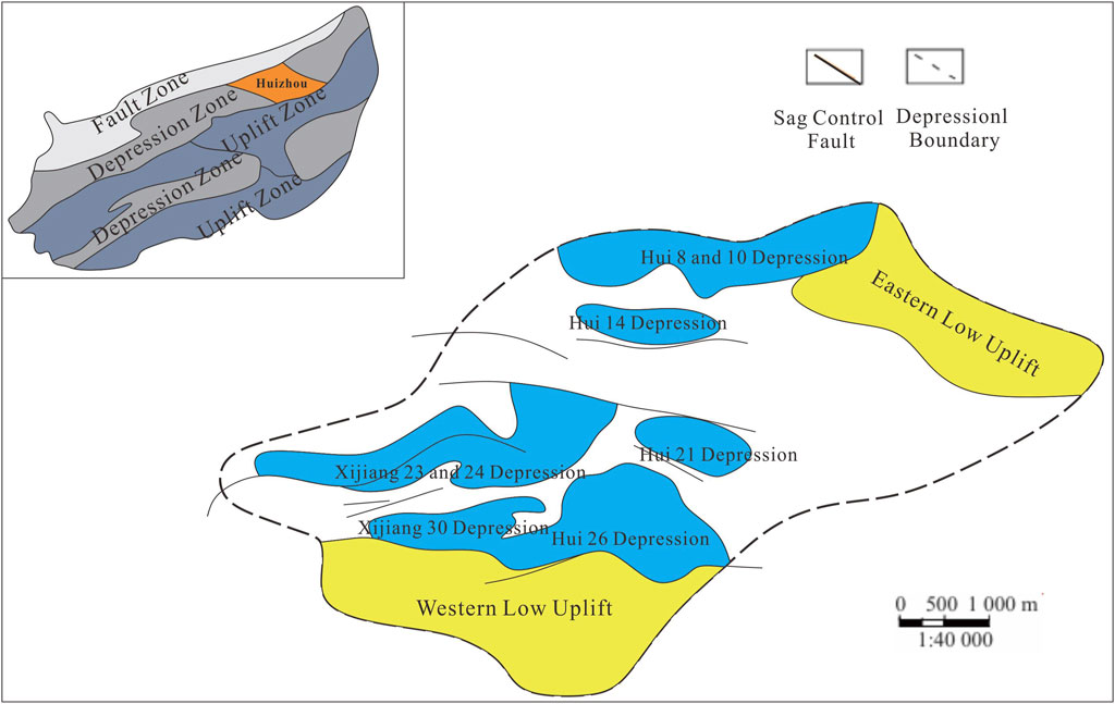
Figure 1. Structural location of Huizhou Oilfield.

The Huizhou Oilfield is located in the southwestern part of the Huizhou Sag, along the southern margin fault zone of the Huizhou 26 Sag. It is a fault-block structural trap formed between two NWW-trending boundary normal faults. The Mesozoic buried-hill lithology primarily consists of intrusive rocks, volcanic eruptive rocks and metamorphic rocks, with reservoir characteristics exhibiting a dual-porosity medium.

Based on the degree of weathering and dissolution modification, the buried hill is vertically subdivided into five zones: the soil layer, hydrolysis zone, leaching zone, collapse zone and bedrock zone. The soil layer, located at the top of the weathering and dissolution zone, consists of mineral particles, organic matter, water, and air. Below the soil layer is the hydrolysis zone, which is characterized by significant chemical changes, especially hydrolysis. In this process, water reacts with minerals, leading to changes in mineral structures and the formation of new minerals. Beneath the hydrolysis zone lies the leaching zone, where soluble substances are dissolved and transported downward by rainwater or other water sources. This results in the loss of certain elements and compounds from this layer, and may also lead to the formation of secondary minerals during the process. Below the leaching zone is the disintegration zone, which is characterized by the physical breakdown and fragmentation of rock, although it has not yet undergone extensive chemical alteration. The bedrock zone is the lowest part of the weathering and dissolution profile and essentially retains the original structure and composition of the rock.

Among these, the leaching zone and collapse zone serve as the primary favorable reservoirs. The collapse zone, having undergone intense weathering and leaching, is characterized by well-developed fractures and dissolution cavities, forming a pore-fracture-type reservoir. In contrast, the leaching zone has experienced relatively weaker weathering and dissolution, predominantly developing fracture-type reservoirs.

The hydrocarbon accumulation in the oilfield is characterized by a “gas cap above, oil below” structural model, forming a block-shaped gas-cap oil reservoir. The upper section contains a condensate gas cap with high condensate oil content, while the lower section comprises a light volatile oil reservoir. Multiple phases of tectonic movements and weathering-dissolution processes have resulted in significant differences in fracture formation potential across various lithologies, leading to strong randomness in the spatial distribution of fractures (Table 1). Therefore, investigating the fracture characteristics and controlling factors of the igneous buried-hill reservoir in the Huizhou Oilfield is crucial for assessing reservoir quality and development potential, ultimately guiding the formulation of effective development strategies.

Table 1

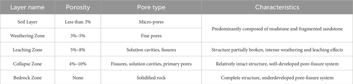
Table 1. Porosity and pore type characteristics of weathering zone.

3 Methods

3.1 Image segmentation based on K-means algorithm and morphological processing

Imaging logging images serve as a crucial data source for fracture identification. However, accurately extracting fracture information directly from these images poses significant challenges, as they typically contain substantial noise, and different types of fractures may exhibit similar visual characteristics (Chai et al., 2025). Therefore, preprocessing of imaging logging images is necessary before performing image segmentation. Subsequently, morphological operations are applied to refine the segmented results and extract fracture features, thereby laying the foundation for subsequent fracture identification (Wu and Gai, 2025).

K-means clustering is a classical unsupervised learning algorithm designed to partition a dataset into K mutually exclusive clusters, ensuring that each data point is assigned to the cluster whose centroid is the closest. The objective is to achieve high intra-cluster similarity and low inter-cluster similarity (Deng et al., 2025). The core principle of the algorithm involves an iterative optimization process that minimizes the sum of squared distances between each sample and its corresponding cluster centroid. Mathematically, this objective is expressed as:

$\mathrm{J}={\displaystyle \sum _{\mathrm{K}=1}^{\mathrm{K}}}{\displaystyle \sum _{\text{x∈}{\text{c}}_{\text{k\hspace{0.17em}}}}}{‖\mathrm{x},–,{\mu }_{\text{k}}‖}^2(1)$

Which ${\mathrm{\mu }}_{\mathrm{k}}$ represents the centroid of the k cluster, and let ${\mathrm{C}}_{\mathrm{k}}$ denote the set of data points belonging to this cluster. The algorithm achieves its objective through an iterative optimization process. Initially, K centroids are randomly initialized. Then, the following two steps are alternately executed until convergence. Assignment Step, each data point is assigned to the cluster whose centroid is closest, based on a distance metric. Update Step, the centroids are recalculated as the mean of all data points within each cluster (Zhang Y. et al., 2025). This process essentially follows a coordinate descent approach, where the algorithm alternates between optimizing cluster assignments and updating centroid positions, progressively minimizing the objective function J until the centroid movement approaches zero.

The figure below (Figure 2) illustrates the principle of the K-means clustering algorithm. Initially, three cluster centroids (red, green and blue) are randomly selected. The distance from each data point to these centroids is computed, and each point is assigned to the nearest cluster (Ji et al., 2024; Ping, 2024). The bold points represent the initial centroids. Next, the cluster centroids are updated by computing the mean of all data points within each cluster. Since the newly computed centroids have shifted, data points are reassigned based on updated Euclidean distances. This process is repeated iteratively until the centroids stabilize or a predefined stopping criterion is met.

Figure 2

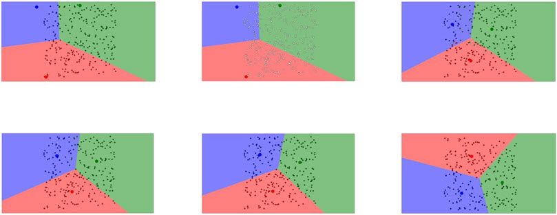
Figure 2. Process diagram of K-means algorithm.

In a color image, each pixel represents a point in a three-dimensional space, where the three dimensions correspond to the intensity values of the red, green and blue (RGB) color channels. The K-means clustering-based image segmentation algorithm treats image pixels as individual data points and clusters them according to a predefined number of clusters (Li et al., 2023; Reddy et al., 2022; Shaf et al., 2021). Each pixel is then replaced with the centroid of its corresponding cluster, thereby reconstructing the segmented image. Morphological image processing is an image analysis technique based on mathematical morphology, primarily used to extract shape-related information from an image. Its fundamental concept is derived from set theory operations, wherein a structuring element is defined and applied to the image through specific logical operations, such as expansion, erosion, opening and closing (Dong et al., 2020). These operations facilitate the analysis and modification of object shapes within the image. In this study, the closing operation is applied after image segmentation to refine the extracted fracture features.

The basic principle of the closing operation involves applying dilation followed by erosion. This process employs a small binary image, known as a structuring element, to interact with the target image. First, dilation is performed, which expands the foreground objects in the image—particularly extending their boundaries outward. At each pixel position, if any neighboring pixel belongs to the foreground, the pixel is marked as foreground (Kölbel et al., 2020). This step helps fill small gaps or fractures within the foreground region, connect closely positioned objects and smoothen irregular boundaries.

Following dilation, erosion is applied to the expanded image. Erosion performs the inverse function by shrinking the foreground objects, specifically removing relatively isolated or boundary pixels. At each pixel location, only those whose entire neighborhood belongs to the foreground are retained as foreground pixels. This step eliminates excessive expansion effects introduced by dilation while preserving the filled gaps and connected structures (Aghli et al., 2020). The figure below (Figure 3) illustrates the principle of the morphological closing operation, where the white region represents the background, and the gray region denotes the foreground objects.

Figure 3

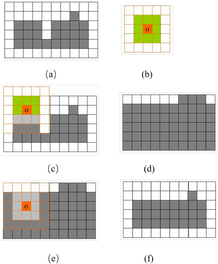
Figure 3. Flow chart of morphological closed operation: (a) original image, (b) structure element, (c) expansive operation, (d) expanded image, (e) erosive operation, (f) result image after corrosion.

When processing imaging logging images, our objective is to extract the dark fracture regions while treating all other areas as the background, thereby performing binary classification between fractures and the background (Park et al., 2020). The process begins by loading the original imaging logging image and converting it to grayscale. To reduce noise, techniques such as Gaussian blur are applied. Next, the image is transformed into a one-dimensional pixel array, and the K-means clustering algorithm is employed to differentiate between the fracture and background regions. Based on the clustering results, the label array is reshaped to reconstruct the segmented image, followed by binarization to enhance the visibility of the fracture regions. To further optimize the segmentation results, morphological closing operations are applied to fill small gaps and connect discontinuous fracture segments. Finally, visualization tools are used to display both the original image and the segmented fracture image, providing an intuitive representation of the fracture detection results.

Through this approach, the K-means clustering algorithm effectively reduces noise in imaging logging images, enhances image quality, and establishes a solid data foundation for subsequent fracture identification.

3.2 Fracture identification based on deep neural network model

Neural network models are inspired by biological neurons. In biological neural cells, synapses receive signals, process them, and determine the signal strength to trigger different neural potential responses. Based on this mechanism, the fundamental structure of neural network models was designed, leading to the development of the neuron model. The figure below (Figure 4) illustrates the simplest neuron model, which was first proposed in 1943 and has been widely used ever since (Zhang et al., 2019).

Figure 4

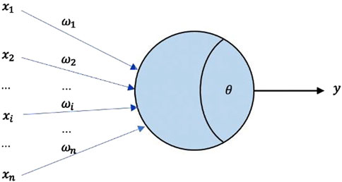
Figure 4. Neuron model.

From the schematic diagram of the model, for a single neuron model, where $\left\{x_1,x_2,......,x_n\right\}$ represents the input data of the model, $\left\{{\omega }_1,{\omega }_2,......,{\omega }_n\right\}$ are the computational parameters of the neuron model, corresponding one-to-one with the dimensions of the input data, used to reflect the weights of each dimension of the input data; $\theta$ denotes the threshold of the neuron output, commonly used to control whether the neuron outputs a result or modifies the output result; $y$ is the output result of the neuron model, calculated as follows:

$y=f\left({\displaystyle \sum _{i=1}^n}{\omega }_i{x}_i-\theta \right)(2)$

The function $f$ is used to map function values to the range [0,1]. This function is commonly referred to as the activation function. To enhance the adaptability of neurons, multiple neurons can be connected to form an artificial neural network.

DNN is a multi-layered artificial neural network model. The fundamental structure of a DNN consists of an input layer, multiple hidden layers and an output layer. The input layer receives external data features, while the hidden layers comprise a series of nonlinear processing units. These units generate new outputs by performing a weighted summation of the previous layer’s outputs followed by an activation function transformation. The output layer produces the final prediction results according to the task requirements. In domains such as image recognition and speech recognition, DNN leverage their hierarchical structure to capture intricate patterns within data.

The DNN first propagates input data forward through the network, performing weighted summation and activation function transformations at each layer until the output layer generates the final prediction. A loss function is then used to measure the difference between the predicted and actual values. Subsequently, the backpropagation algorithm computes the gradient of each layer and updates the weights using an optimization algorithm to minimize the loss function (Shi et al., 2018). This process iterates continuously until the model converges or reaches a predefined number of training epochs. To enhance model performance and prevent overfitting, DNN incorporate several key techniques, including activation functions to increase nonlinear representational capacity, regularization methods to reduce model complexity, and batch normalization to accelerate the training process (Zhou et al., 2017). Through multi-layer nonlinear transformations, DNN can automatically extract high-level features from data, enabling effective learning and prediction of complex patterns (Tian et al., 2021).

4 Results

4.1 Segmentation result

First, the original imaging logging image is loaded and read in grayscale mode. A Gaussian blur filter with a kernel size of $5\times 5$ is then applied for noise reduction. Next, the image is reshaped into a one-dimensional pixel array, and the K-means clustering algorithm (with the number of clusters set to k = 2) is used to distinguish fractures from the background. After clustering is completed, the label array is reshaped back to match the original image dimensions, producing the segmented image. A binarization process is then applied, where the fracture regions are marked in black and the background in white. To further enhance the representation of fracture regions, morphological closing operations are employed to fill small voids and connect fragmented areas. Finally, the original image and the fracture segmentation results are visualized using the Matplotlib library, providing an intuitive representation of the fracture detection outcome. The following figure (Figure 5) illustrates the segmentation workflow.

Figure 5

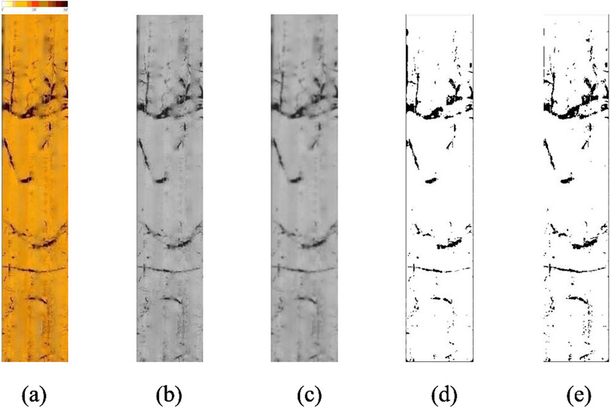
Figure 5. Flow chart of image segmentation: (a) original image (3984–3989 m), (b) grayscale image, (c) denoising grayscale image, (d) K-means segmentation image, (e) morphological processing results image.

To intuitively demonstrate the advantages of the K-means algorithm and morphological operations, imaging logging images were also processed using traditional Otsu threshold segmentation and CNN-based machine learning image segmentation. The results are shown in the figure below (Figure 6).

Figure 6

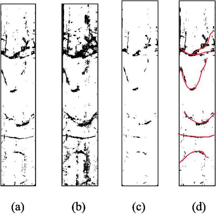
Figure 6. Comparison of different segmentation methods: (a) K-means and morphological, (b) Otsu, (c) CNN, (d) Artificial fracture calibration.

The Otsu method tends to select an overly large foreground area when segmenting images, and it also results in a relatively high number of noise points. This leads to extracted fracture features being not clearly defined. CNN-based image segmentation methods are currently widely used and yield better results, especially due to their strong performance in feature extraction. However, under the condition of small sample sizes, CNN models often suffer from insufficient training data, which reduces machine learning efficiency and negatively affects segmentation outcomes. In practice, this manifests as significant over-segmentation, increasing the difficulty of subsequent fracture identification. Other segmentation algorithms, such as edge detection and region growing, also tend to perform poorly in practical applications. By applying image segmentation based on the K-means algorithm, imaging logging images were successfully processed. This method significantly improved the distinguishability between fracture regions and the background, reduced noise interference, and made fracture outlines clearer. Especially for fracture identification within small sample datasets, this approach demonstrated notable advantages.

The K-means algorithm clusters pixel values into two classes. During processing, the original image is first converted into a grayscale image, and Gaussian blur is applied to reduce noise. Then, the K-means algorithm segments the image by assigning each pixel to the nearest cluster center, thereby distinguishing the fracture regions from the background. This process effectively enhances the fracture outlines. After K-means segmentation, morphological closing operations are applied to fill small gaps and connect discontinuous fracture segments. This step is particularly useful for removing artifacts caused by weathering or other geological processes, as it helps fill minor gaps within fractures while preserving the overall structure of the fractures.

To quantitatively evaluate the effectiveness of fracture segmentation and extraction, the Jaccard Index was introduced. The formula is defined as $J\left(A,B\right)=\frac{\left|A\cap B\right|}{\left|A\cup B\right|}$, where A and B represent the segmented result image and the actual fracture region image, respectively. The value ranges from 0 to 1, with 1 indicating a perfect match. The table below (Table 2) shows the Jaccard Index values obtained using different segmentation methods.

Table 2

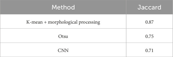
Table 2. Comparison of segmentation effects using different methods.

Specifically, in the application case of the Huizhou Oilfield, multiple drilling samples were tested, revealing that this method successfully differentiates various types of fractures, including dissolution fracture, semi-open fracture and continuous fracture. These fractures not only exhibit morphological differences but also vary in their distribution and development. Continuous fracture typically appear as continuous dark sinusoidal curves or bands, particularly prominent in high-angle or vertical orientations. When unfilled, these fractures exhibit large apertures with well-defined boundaries, whereas the presence of low-resistivity mud or mineral filling results in dark streaks. Continuous fractures often interweave with other fractures to form a network structure, enhancing reservoir connectivity. Semi-open fracture appear as incomplete sinusoidal curves or discontinuous dark streaks. Their open and filled sections display different resistivity characteristics due to variations in material composition. The filling degree typically ranges from 20% to 50%, and dissolution marks may be present. Dissolution fracture, on the other hand, appear in imaging logging as irregular dark spots or bead-like structures with a wide range of width variations. Their edges are jagged, often accompanied by dissolution cavities, forming a network or honeycomb structure. These fractures are usually unfilled or partially filled, with a notable characteristic of reduced resistivity, which aids in identifying high-quality reservoirs. The figure below (Figure 7) presents a comparative analysis of the three typical fracture morphologies after image segmentation, and the quantitative criteria for fracture classification (Table 3).

Figure 7

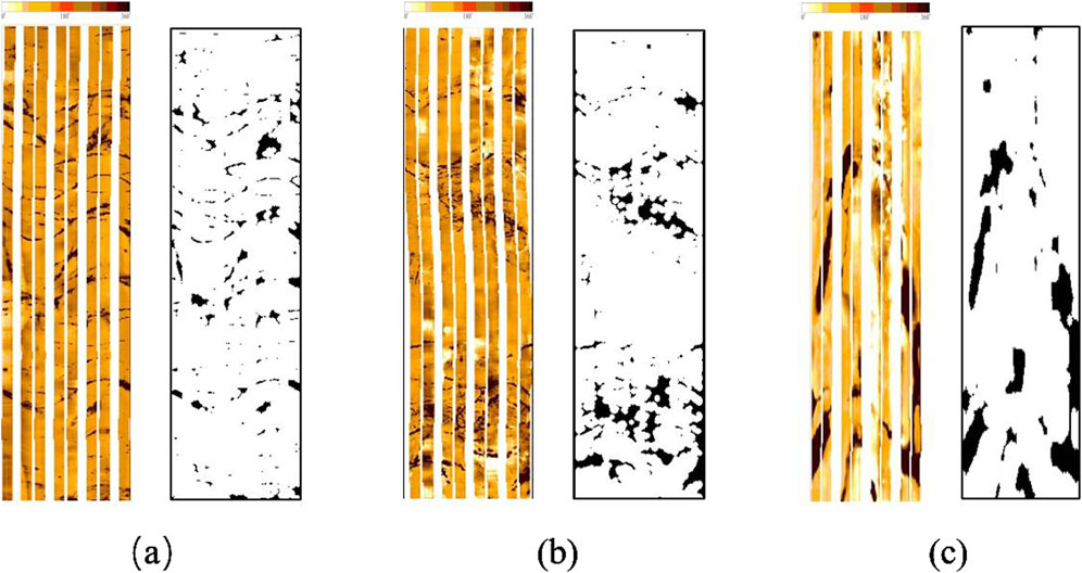
Figure 7. Comparison of different fracture: (a) continuous fracture (3742–3745 m), (b) semi-open fracture (3320–3323 m), (c) dissolution fracture (3805–3808 m).

Table 3

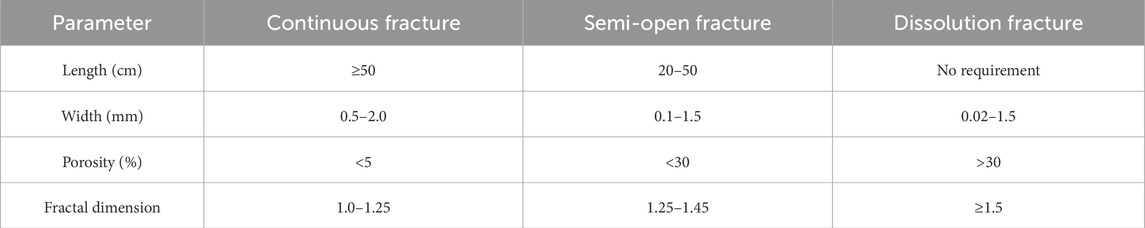
Table 3. Quantitative table of different fracture parameters.

4.2 Detection result

During the fracture identification stage, DNN model is employed to process the optimally segmented images. Leveraging the powerful learning capability of DNN, the model can automatically extract and classify different types of fractures. After completing image segmentation and obtaining high-quality pore-fracture images, a DNN model is constructed for pore-fracture identification. First, the input layer consists of 20 neurons, each corresponding to a specific image feature, such as fracture length, fracture width, fracture angle, curvature and fractal dimension. Next, the model is designed with three hidden layers: the first layer contains 10 neurons, the second layer contains 5 neurons, and the third layer contains 3 neurons (3-layer fully connected (FC) network, with 10, 5, and 3 neurons respectively). The ReLU activation function is applied between layers to accelerate convergence and mitigate the vanishing gradient problem. Finally, the output layer consists of a single neuron, utilizing an 8-fold Sigmoid activation function to map the output to the range [0,8]. The mathematical expression is given by:

$\text{Output}=8\times \sigma \left(z\right)=\frac{8}{1+e^{-z}}(3)$

where $z$ represents the weighted input value of the output layer. To optimize model learning, the labels are mapped to the midpoint values of their corresponding intervals based on fracture types. Specifically, continuous fracture [0,2) are assigned a label value of 1.0; semi-open fracture [2,4) are assigned a label value of 3.0; dissolution fracture [4,6) are assigned a label value of 5.0; and non-pore fracture [6,8) are assigned a label value of 7.0. The labeled fracture images, along with their morphological features and corresponding label values, are paired as training data. The mean squared error (MSE) is used as the loss function to measure the discrepancy between the predicted and actual labels. MSE is sensitive to deviations from the target values, making it well-suited for regression tasks, as it effectively drives the model output toward the midpoint values of the assigned labels.

$\text{Loss}=\frac{1}{N}{\displaystyle \sum _{i=1}^N}{\left(y_{\text{pred}}^{\left(i\right)}-y_{\text{true}}^{\left(i\right)}\right)}^2(4)$

In the equation, Loss represents the loss or error between the model’s predicted results and the actual results. $N$ denotes the number of samples in the training dataset. $y_{\text{pred}}^{\left(i\right)}$ represents the predicted value of the i sample, while $y_{\text{true}}^{\left(i\right)}$ denotes the actual value of the i sample. The figure below (Figure 8) illustrates the conceptual structure of the DNN model used in this study.

Figure 8

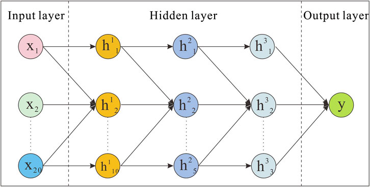
Figure 8. DNN model principle figure.

To train this model, a total of 100 sample images (50 Continuous fractures, 33 Semi-open fractures, 17 Dissolution fractures) were randomly divided into 70 images for training and 30 images for testing. In each iteration, the images from the training set were fed into the model, and the predicted values were computed through forward propagation. Specifically, the input layer received image features and propagated them through multiple hidden layers, where each layer applied a linear transformation followed by the ReLU activation function. This process continued until the final hidden layer’s output was passed to the output layer, generating the final prediction. The predicted values were then compared with the actual labels to compute the loss. Subsequently, the backpropagation algorithm was employed to compute the gradients of the loss function with respect to the weights and biases of each layer. An optimization algorithm was then used to update these parameters, minimizing the loss function. The training configuration includes the Adam optimizer (learning rate = 0.001, β1 = 0.9, β2 = 0.999). In the case of a small training dataset, the batch size is set to 16, and regularization is applied using L2 weight decay (λ = 0.01) combined with Dropout (hidden layer probability = 0.2). Training is terminated if the validation loss does not decrease for five consecutive epochs. Five-fold cross-validation is used to optimize the hidden layer structure (number of layers: 2–5, neurons per layer: 5–20). The learning rate grid search range is {0.1, 0.01, 0.001}. The optimal configuration obtained was a 3-layer network (with 10, 5, and 3 neurons respectively) and a learning rate of 0.001.

Through multiple iterations, the model progressively optimized its parameters, improving its recognition accuracy. After training, the model’s performance was evaluated using the test set to ensure its generalization ability. Ultimately, the trained model could be applied to new imaging logging images, automatically identifying and classifying different types of pore-fracture structures (Table 4), thereby significantly enhancing the overall accuracy of pore-fracture recognition.

Table 4

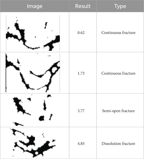
Table 4. Result table of fracture detection.

5 Discussion

This method was applied to the fracture identification task in the buried hill reservoir of the Huizhou Oilfield. Through testing on multiple samples, its effectiveness and reliability were validated. Experimental results demonstrated that in addressing fracture identification in low-permeability reservoirs, this method not only improved recognition accuracy but also enhanced the understanding of complex geological structures. To further verify the practical applicability of the model, a 5-m segment was randomly extracted from a 682-m-long imaging logging image. The goal was for the model to automatically identify different pore-fracture structures within this segment and determine their corresponding well depths. First, the 5-m image was divided into regions. Since the grayscale values of the regions containing pore-fractures significantly differed from other regions, the segmentation process was primarily based on grayscale variations. Ultimately, the image was divided into seven sub-images, each containing distinct geological features, thereby providing fundamental data for subsequent pore-fracture identification.

After completing the segmentation, these seven sub-images were input into the pre-trained deep neural network model for pore-fracture identification. Among the seven sub-images, two contained continuous fractures, four contained semi-open fracture, and one contained dissolution fracture. The final identification results are shown in the figure below (Figure 9). The penultimate column represents the manually annotated fracture type, while the last column indicates the fracture type identified by the model.

Figure 9

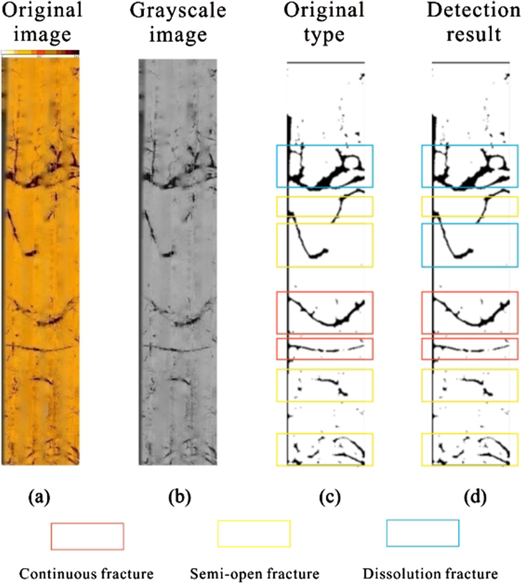
Figure 9. Detection result figure: (a) original image (3984–3989 m), (b) grayscale image, (c) manually annotated result, (d) DNN fracture detection result.

Through model identification, the continuous fracture and vuggy fracture were successfully recognized. However, there was one misclassification in the identification of a semi-open fracture, where the detected fracture type did not match the original annotation. The primary reason for this misclassification is that the features of the semi-open fracture in this sample image were not distinct, with either a relatively large fracture width or discontinuous structure, leading the model to misclassify it as a dissolution fracture.

To validate the classification performance of the model, we conducted a quantitative comparison between this method and the traditional methods commonly used in the Huizhou Oilfield. The results are shown in the table below (Tables 5, 6).

Table 5

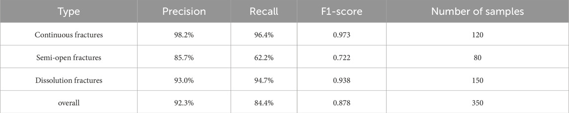
Table 5. Accuracy parameter table of different fracture types.

Table 6

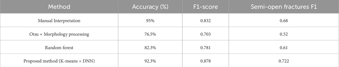
Table 6. Accuracy comparison table of different methods.

The results indicate that accuracy and F1-Score are very high for the identification of continuous fractures and dissolution fractures, while relatively lower for semi-open fractures. There are multiple instances where areas of semi-open fractures were misidentified as dissolution fracture structures in the images. The main reason is still due to the lack of distinct features of semi-open fractures, making feature extraction more challenging during model training compared to continuous and dissolution fractures. The model has certain limitations when dealing with ambiguous or indistinct geological structures. Compared with traditional methods, our approach not only excels in overall accuracy and F1-Score but also shows competitiveness in processing speed. In future research, we aim to further improve the recognition accuracy for semi-open fractures by increasing the sample size and adding more feature parameters.

Based on the fractures identified by the DNN model, to further characterize the reservoir properties, quantitative fracture parameters were extracted.

Fracture density: Calculated as the total number of fractures per unit area. This parameter reflects the intensity of fracture development and is obtained by summing all fractures in the segmented images and dividing by the image area; Fracture aperture: Measured in the imaging logging images as the average width of the fracture traces. Pixel-level analysis of the binarized fracture regions was performed, followed by an analysis considering the borehole diameter from imaging logging; Fracture dip angle: Determined by fitting sinusoidal curves to continuous fractures and calculating the angle between the fracture plane and the horizontal axis. For non-sinusoidal fractures, geometric orientation analysis using the Hough transform was applied.

These parameters underwent statistical analysis across multiple samples. Continuous fractures exhibit high dip angles (40°–80°) and large apertures (0.5–2.0 mm), whereas dissolution fractures show lower dip angles (10°–30°) with variable apertures (0.02–1.5 mm). Semi-open fractures display intermediate characteristics. Using these extracted fracture parameters, reservoirs were classified into three categories based on density, aperture, and dip angle.

High-efficiency fracture reservoir (Ⅰ): Dominated by continuous fractures, characterized by high fracture density (>2.5 m/m²), medium to large apertures (>1.0 mm), and good connectivity of the fracture network. These areas are associated with collapse and leaching zones; Moderate fracture-pore reservoir (Ⅱ): Characterized by a mixture of semi-open fractures and dissolution fractures, with moderate fracture density (1.5–2.5 m/m²), small to medium apertures (0.5–1.0 mm), and partial connectivity. They are mainly found in the transitional zone between weathering and leaching layers; Low-efficiency tight reservoir (Ⅲ): Predominantly isolated dissolution cavities or micro-fractures, low fracture density (<1.5 m/m²), narrow apertures (<0.5 mm), and isolated fractures. These are typically associated with bedrock and soil layers.

The following figure (Figure 10) is a cross plot of fracture density versus aperture, visually illustrating the classification criteria. High-efficiency fracture reservoirs cluster in the upper right quadrant, while low-efficiency tight reservoirs occupy the lower left region.

Figure 10

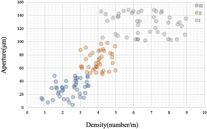
Figure 10. The crossplot of fracture density and aperture.

The results indicate that fracture parameters directly influence reservoir permeability and storage capacity, thereby controlling fluid flow efficiency. High-efficiency fracture reservoirs, characterized by abundant interconnected fractures, become the primary targets for hydraulic fracturing. This quantitative relationship provides a data-driven foundation for optimizing development strategies and enhancing recovery efficiency in complex buried-hill reservoirs.

The following figure (Figure 11) is the intersection diagram of fracture characteristic parameters and production.

Figure 11

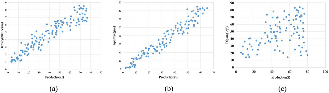
Figure 11. The crossplot of fracture parameters and production, (a) The crossplot of fracture density and production; (b) The crossplot of fracture aperture and production; (c) The crossplot of fracture dip angle and production.

The above figure shows that fracture density, aperture and production have significant correlation, and fracture dip angle has better correlation at low angle and weaker correlation at high angle. The following table (Table 7) is the different types of fracture reservoirs and fracture parameters value.

Table 7

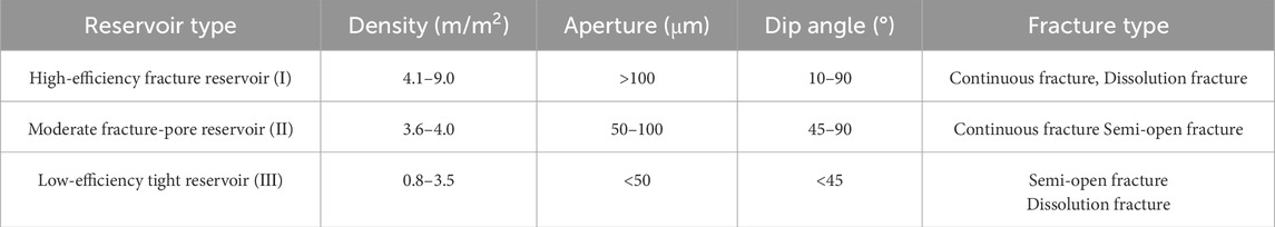
Table 7. Table of different types of fracture reservoirs.

6 Conclusion

(1) Through the combination of the K-means algorithm and morphological operations, the separation between fracture regions and the background has been significantly improved, making this method particularly suitable for fracture identification under complex geological conditions. This approach effectively reduces noise interference and enhances the clarity of fracture contours, providing high-quality input data for subsequent identification.

(2) By leveraging the powerful learning capabilities and automatic feature extraction of DNN, high-precision identification of different types of fractures has been achieved.

(3) This method has achieved excellent results in practical applications within the Huizhou Oilfield, with an overall accuracy of fracture extraction and identification exceeding 90%. It establishes a quantitative bridge between fracture characteristics and production performance by extracting fracture parameters and classifying reservoirs, thereby enhancing the practical value of fracture recognition.

(4) Future work will focus on improving model accuracy through data augmentation and the integration of multiple imaging techniques, as well as exploring optimizations of different deep learning architectures. By employing cross-domain transfer learning and dynamic adjustment mechanisms to enhance adaptability, we aim to achieve more precise fracture identification in complex geological structures. This will provide new insights for related technologies.

Data availability statement

The original contributions presented in the study are included in the article/supplementary material, further inquiries can be directed to the corresponding author.

Author contributions

MW: Writing – original draft, Writing – review and editing. QZ: Writing – original draft, Writing – review and editing. LY: Writing – original draft, Writing – review and editing. YD: Writing – original draft, Writing – review and editing.

Funding

The author(s) declare that no financial support was received for the research and/or publication of this article.

Conflict of interest

Authors MW, QZ, LY, and YD were employed by China Oilfield Services Limited.

Generative AI statement

The author(s) declare that no Generative AI was used in the creation of this manuscript.

Publisher’s note

All claims expressed in this article are solely those of the authors and do not necessarily represent those of their affiliated organizations, or those of the publisher, the editors and the reviewers. Any product that may be evaluated in this article, or claim that may be made by its manufacturer, is not guaranteed or endorsed by the publisher.

References

Aghli, G., Moussavi-Harami, R., and Tokhmechi, B. (2020). Integration of sonic and resistivity conventional logs for identification of fracture parameters in the carbonate reservoirs (A case study, carbonate Asmari formation, Zagros basin, SW Iran). J. Petroleum Sci. Eng. 186, 106728. doi:10.1016/j.petrol.2019.106728

CrossRef Full Text | Google Scholar

Chai, X., Wu, Z., Li, W., Fan, H., Sun, X., and Xu, J. (2025). Image segmentation based on the optimized K-Means algorithm with the improved hybrid grey wolf optimization: application in ore particle size detection. Sensors 25 (9), 2785. doi:10.3390/s25092785

PubMed Abstract | CrossRef Full Text | Google Scholar

Deng, G., Sun, H., and Xie, W. (2025). Correlation-based switching mean teacher for semi-supervised medical image segmentation. Neurocomputing 633, 129818. doi:10.1016/j.neucom.2025.129818

CrossRef Full Text | Google Scholar

Ding, W., Xu, C., and Jiu, K. (2011). The research progress of shale fractures. Adv. Earth Sci. 26, 135–144.

Google Scholar

Dong, S., Zeng, L., Liu, J., Gao, A., Lyu, W., Du, X., et al. (2020). Fracture identification in tight reservoirs by multiple kernel fisher discriminant analysis using conventional logs. Interpretation 8 (4), 215–225. doi:10.1190/int-2020-0048.1

CrossRef Full Text | Google Scholar

Hu, J., Tong, D., Song, Y., and Yu, Z. (2025). Modified possibilistic fuzzy C-means clustering driven by weighted residuals for image segmentation. J. Phys. Conf. Ser. 3004 (1), 012004. doi:10.1088/1742-6596/3004/1/012004

CrossRef Full Text | Google Scholar

Ji, C., Dong, S., Zeng, L., Liu, Y., Hao, J., and Yang, Z. (2024). Fracture identification of carbonate reservoirs by deep forest model: an example from the D oilfield in Zagros basin. Energy Geosci. 5 (3), 100300. doi:10.1016/j.engeos.2024.100300

CrossRef Full Text | Google Scholar

Kölbel, L., Kölbel, T., Sauter, M., Schäfer, T., Siefert, D., and Wiegand, B. (2020). Identification of fracture zones in geothermal reservoirs in sedimentary basins: a radionuclide-based approach. Geothermics 85, 101764. doi:10.1016/j.geothermics.2019.101764

CrossRef Full Text | Google Scholar

Li, J., Dunqing, X., and Guoquan, L. (2007). Method evaluating micritic calcite dolomite reservoirs in west slope of Qikou Sag of Huanghua depression and its application. China Pet. Explor. 12 (5), 55.

Google Scholar

Li, S., Tang, X., and He, J. (2020). Fracture characterization combining acoustic reflection imaging and rock mechanics. Acta Pet. Sin. 41, 1388.

Google Scholar

Li, Z., Li, X., Dai, W., Yikai, Z., Lingxia, Z., and Liwu, M. (2023). Fracture identification and its application of ultra-low permeability carbonate reservoir in Fauqi North oilField, Iraq. Arabian J. Geosciences 16 (11), 623. doi:10.1007/s12517-023-11738-x

CrossRef Full Text | Google Scholar

Lina, Y., Bin, Y., and Hongjiang, L. (2011). Prediction of fracture development in changxing formation reservoir of wubaiti gas field from conventional logging data using neural networks. China Pet. Explor. 16, 63.

Google Scholar

Liu, Z., Wang, K., and Bao, Q. (2022). Prediction method of rock physics S-wave velocity in tight sandstone reservoir: a case study of yanchang formation in ordos basin. Acta Pet. Sin. 43, 1284.

Google Scholar

Ming, Z., Jinjie, H., and Xuefeng, B. (2011). Application of fracture prediction with prestack seismic data in Fengcheng field of Junggar basin. China Pet. Explor. 16, 25.

Google Scholar

Park, H. C., Kim, Y. J., and Lee, S. W. (2020). Adenocarcinoma recognition in endoscopy images using optimized convolutional neural networks. Appl. Sci. 10 (5), 1650. doi:10.3390/app10051650

CrossRef Full Text | Google Scholar

Ping, S. (2024). Fracture identification and porosity prediction of carbonate reservoirs based on neural network simulation. E3S Web Conf. 561, 03001. doi:10.1051/e3sconf/202456103001

CrossRef Full Text | Google Scholar

Reddy, S. R. G., Saradhi, G. P., and Lakshmi, D. R. (2022). Deep neural network (DNN) mechanism for identification of diseased and healthy plant leaf images using computer vision. Ann. Data Sci. 11 (1), 243–272. doi:10.1007/s40745-022-00412-w

CrossRef Full Text | Google Scholar

Shafiabadi, M., Rouhani, A. K., and Sajadi, S. M. (2021). Identification of the fractures of carbonate reservoirs and determination of their dips from FMI image logs using Hough transform algorithm. Oil and Gas Sci. Technol. – Revue d’IFP Energies nouvelles 76, 37. doi:10.2516/ogst/2021019

CrossRef Full Text | Google Scholar

Shi, P., Yuan, S., Wang, T., Wang, Y., and Liu, T. (2018). Fracture identification in a tight sandstone reservoir: a seismic anisotropy and automatic multisensitive attribute fusion framework. IEEE Geosci. Remote Sens. Lett. 15 (10), 1525–1529. doi:10.1109/lgrs.2018.2853631

CrossRef Full Text | Google Scholar

Stadtműller, M. (2019). Well logging interpretation methodology for carbonate formation fracture system properties determination. Acta Geophys. 67 (6), 1933–1943. doi:10.1007/s11600-019-00351-w

CrossRef Full Text | Google Scholar

Tian, J., Liu, H., Wang, L., Sima, L., Liu, S., and Liu, X. (2021). Identification of fractures in tight-oil reservoirs: a case study of the Da'anzhai member in the central Sichuan basin, SW China. Sci. Rep. 11 (1), 23846. doi:10.1038/s41598-021-03297-6

PubMed Abstract | CrossRef Full Text | Google Scholar

Wang, G., Zheng, J., and Fan, Z. (2005). Depositional genesis of Anpeng structural nose and fractures distributed in Anpeng deep zones. Acta Pet. Sin. 26 (2), 38.

Google Scholar

Wang, S., Wang, G., Zeng, L., Liu, P., Huang, Y., Li, S., et al. (2025). New method for logging identification of natural fractures in shale reservoirs: the Fengcheng formation of the Mahu Sag, China. Mar. Petroleum Geol. 176, 107346. doi:10.1016/j.marpetgeo.2025.107346

CrossRef Full Text | Google Scholar

Wen, H. (2014). Quantitative identification of reservoir fracture with the variable scale fractal technique in Su53 gas field, ordos basin. Adv. Mater. Res. 3384, 1723–1726. doi:10.4028/www.scientific.net/amr.1010-1012.1723

CrossRef Full Text | Google Scholar

Wu, C., and Gai, P. (2025). A novel joint learning framework combining fuzzy C-multiple-means clustering and spectral clustering for superpixel-based image segmentation. Digit. Signal Process. 161, 105083. doi:10.1016/j.dsp.2025.105083

CrossRef Full Text | Google Scholar

Wu, C., and Guo, M. (2025). A new approach to incorporate log-local information into improved kernel possibilistic C-means clustering with spatial constraints for image segmentation. Multimedia Tools Appl. 1–34. doi:10.1007/s11042-025-20848-5

CrossRef Full Text | Google Scholar

Zhang, J. J., Zhang, G. Z., and Huang, L. H. (2019). Crack fluid identification of shale reservoir based on stress-dependent anisotropy. Appl. Geophys. 16 (2), 209–217. doi:10.1007/s11770-019-0754-5

CrossRef Full Text | Google Scholar

Zhang, H., Ma, P., Liu, J., Lian, J., and Ma, Y. (2025a). Prototype-augmented mean teacher for robust semi-supervised medical image segmentation. Pattern Recognit. 166, 111722. doi:10.1016/j.patcog.2025.111722

CrossRef Full Text | Google Scholar

Zhang, Y., Ma, D., and Wu, X. (2025b). Source-free domain adaptation framework based on confidence constrained mean teacher for fundus image segmentation. Neurocomputing 620, 129262. doi:10.1016/j.neucom.2024.129262

CrossRef Full Text | Google Scholar

Zhou, Y., Fuqiang, L., Lei, X., Liu, L., Yu, T., Chen, J., et al. (2017). Study on fracture identification of shale reservoir based on electrical imaging logging. IOP Conf. Ser. Earth Environ. Sci. 64 (1), 012041. doi:10.1088/1755-1315/64/1/012041

CrossRef Full Text | Google Scholar