Spatiotemporal variability of turbulent fluxes in snow-covered mountain terrain

Turbulent exchange of heat and moisture plays an important role in snow cover dynamics. Although these processes are subject to great spatial and temporal variability, especially in complex terrain, measurements of heat, moisture, and momentum fluxes are almost exclusively point observations. Numerical modeling offers a means to assess the spatial variability of fluxes and evaluate the representativeness of point observations. This study addresses this challenge by examining the spatiotemporal variability of surface–atmosphere energy exchange during different meteorological events in the Swiss Alps using the NWP model CRYOWRF. We analyze sources of errors in representing energy exchange over snow in mountain areas by models. To investigate this, we first compared fluxes derived from Monin-Obukhov parameterizations with direct Eddy Covariance measurements. While the parameterization generally captures the sign of the fluxes, it tends to underestimate their magnitude, up to 20 W ${\text{m}}^{-2}$ for latent heat flux. We then evaluate CRYOWRF—the WRF model coupled with the SNOWPACK land-surface scheme–in representing fluxes and mean quantities. Simulations at 1 km and 200 m resolution are compared against data from 21 meteorological stations in a 40 × 40 km domain in the Swiss Alps during three conditions: a South Föhn, a North Föhn, and a quiescent day. Our findings indicate that while higher-resolution simulations improve agreement between measured and modeled variables, they tend to underestimate wind speeds (with a bias of up to 1.5 $\pm$ 0.2 m ${\text{s}}^{-1}$), and turbulent fluxes (up to 14 $\pm$ 3.7 W ${\text{m}}^{-2}$) and consequently lower snow surface temperatures (up to 3.3 $\pm$ 0.3 °C). In contrast, coarser-resolution simulations overestimate wind speeds, and therefore, heat fluxes. Our research demonstrates that magnitudes of turbulent fluxes scale linearly with local wind speeds (r-values between −0.80 and −0.98 for sensible heat flux on a south föhn day, p-values $<$ 0.001), with locations at similar elevations exhibiting comparable trends of increasing turbulent flux with wind speed. Although temperature and humidity gradients generally decrease with elevation, higher elevations still experience greater net energy exchange between the surface and the atmosphere. A net magnitude increase of 30 W ${\text{m}}^{-2}$ is observed between elevation differences of 1,000 m. Overall, our results suggest that point measurements should be used with caution for representing broader terrain conditions, especially when extrapolated for different elevations.

1 Introduction

Interactions between the atmosphere and the surface play a crucial role in shaping the temporal and spatial evolution of snow cover over mountainous regions. The main drivers of snow ablation are spatially and temporally variable shortwave radiation, longwave radiation, and turbulent exchange of heat and moisture (Mott et al., 2011). Therefore, an accurate representation of turbulent fluxes is essential for modeling the mass and energy balance of snowpacks, which, in turn, is critical for capturing the snow hydrological cycle, avalanche hazards, and climate in cold regions.

Despite the variability of turbulent fluxes over heterogeneous terrain (Lehner and Rotach, 2018), nearly all measurements of turbulent exchange of heat and moisture in snow-atmosphere interactions are point measurements. In-situ measurements of turbulent fluxes are furthermore scarce and, especially in complex terrain, do not represent all terrain types. Recent advances have enabled high-resolution investigations of near-surface atmospheric dynamics using thermal infrared imaging on a small spatial scale of several meters (Haugeneder et al., 2023). This method reveals substantial spatial and temporal variability of near-surface atmospheric quantities and turbulent fluxes over heterogeneous surfaces. However, this method remains unfeasible for large-scale applications, necessitating the use of numerical modeling to improve our understanding of turbulent flux variability.

Computations of turbulent fluxes in numerical weather prediction (NWP) models rely on similarity scaling parameterizations such as the Monin-Obukhov Similarity Theory (MOST), which are based on wind speed, temperature and humidity gradients, and the resulting stability of the atmosphere. These parameterizations assume quasi-stationarity, horizontal homogeneity, and the presence of a constant-flux layer near the surface (Foken, 2006) - assumptions that are never fulfilled in highly complex terrain. Despite this, MOST is still widely applied in such environments, even though it was originally developed for flat, homogeneous surfaces (Rotach and Zardi, 2007). At coarser resolutions, smoother representations of topography tend to uphold the assumptions underlying MOST (Epifanio, 2007). However, as model resolution increases and terrain complexity is more explicitly resolved, the limitations of traditional approaches become more pronounced (Goger et al., 2016). In such cases, improved representations of turbulent fluxes, such as the generalized extension of MOST proposed by Stiperski and Calaf (2023), offer a more robust framework for capturing turbulent fluxes in heterogeneous and complex terrain—but these frameworks have not yet been applied in NWP models.

Furthermore, snow-covered surfaces strongly influence the character of the boundary layer, leading to the development of highly stable boundary layers due to radiative cooling or advection of warm air over a colder surface (Schlögl et al., 2017) in combination with a smoother snow surface. In such conditions, turbulence weakens, and surface layer decoupling can occur. These stably stratified boundary layers, which remain less well understood than their unstable counterparts (Mahrt, 2014), pose an additional challenge for NWP models, as they are often associated with excessive cooling biases (Zheng et al., 2017).

In summary, the two-way interactions between surface and atmosphere, especially in complex terrain and stable boundary layers, pose significant challenges for NWP models (Goger et al., 2022). Nonetheless, we rely on NWP models for their accurate representations of turbulent fluxes, which are critical for weather forecasting, avalanche prediction, and hydrological assessments. Turbulent fluxes, for instance, are among the key drivers of spring snowmelt (Mott et al., 2011). One key to correctly deriving turbulent fluxes is to accurately represent the wind field in heterogeneous topography (Mott et al., 2018). The diurnal cycle of wind fields is generally well-understood and effectively modeled over complex terrain. However, the question remains of how well the turbulent fluxes are represented in NWP models in these environments.

Although previous studies have examined the spatial variability of turbulent fluxes, they have primarily focused on melting events for hydrological applications (Pohl et al., 2006) and on patchy snow cover dynamics (Mott et al., 2015; Haugeneder et al., 2023; Mott et al., 2017; Schlögl et al., 2018). Additionally, many atmospheric models employ a simplified, single-layer representation of the snowpack, limiting their ability to capture complex snow-atmosphere interactions. Recent developments in fully coupled atmosphere-snowpack models, such as Meso-NH/Crocus (Vionnet et al., 2014), RACMO (Gadde and van de Berg, 2024), and CRYOWRF (Sharma et al., 2021), have improved the representation of these interactions and even implemented blowing snow schemes, which allow enhanced sublimation. In CRYOWRF, meteorological variables computed by the atmospheric component are directly coupled to the physics-based, multi-layer snow cover model SNOWPACK (Lehning et al., 1999; Lehning et al., 2002), which computes the turbulent fluxes. However, a gap remains in the literature concerning the spatial variability of turbulent sensible and latent heat fluxes within these fully coupled models, especially at high resolutions typical of modern NWP applications over complex terrain. Particularly research during synoptic flow-induced weather patterns in mountain regions, such as föhn, remains limited (Gohm et al., 2004).

To address this gap, the present study aims to enhance our understanding of turbulent flux variability over snow-covered mountainous terrain, using the state-of-the-art model CRYOWRF. We focus on three distinct synoptic weather patterns characteristic of the Alps: south föhn, north föhn, and calm high-pressure conditions. A key objective of this study is to assess the representativeness of point measurements of turbulent fluxes for an entire terrain and to understand how these fluxes vary spatially. To achieve this, we first compare CRYOWRF simulations to point measurements of turbulent fluxes in complex terrain, evaluating whether the model accurately represents fluxes given uncertainties in input variables and parameterizations. This allows us to examine the effect of model resolution on turbulent flux predictions, specifically comparing resolutions of 1 km and 200 m. Next, we analyze the temporal variability of turbulent fluxes across the terrain, with a particular focus on the differences induced by varying synoptic weather patterns. Finally, we investigate the influence of key topographical features on turbulent fluxes, identifying the dominant features that drive spatial variability.

2 Methods

2.1 Measurement sites and instrumentation

The study area is located in the Eastern Swiss Alps, in the mountainous region surrounding Davos, Switzerland. This area is characterized by complex alpine terrain and is predominantly snow-covered in winter. The area covers altitudes from 480 to 3,080 m a.s.l. It also benefits from an abundance of meteorological measurements.

We use two types of measurement stations in this study: a primary research site with eddy covariance (EC) instrumentation and 20 supplementary conventional meteorological stations. The main site is the Weissfluhjoch (WFJ) research station, operated by the Snow and Avalanche Research Institute (SLF). This site is extensively used for avalanche and snow research and includes both low- and high-frequency measurements.

The supplementary stations belong to the Inter-Cantonal Measurement and Information System (IMIS) network (Lehning et al., 1999) and include additional research stations at Wannengrat and Laret. These stations provide low-frequency meteorological data.

Figure 1 presents an overview map showing the locations of all field sites. Wind roses at selected stations illustrate the local wind climate, revealing significant variation in mean wind direction across the region. This variability indicates that thermally and terrain-driven circulations (e.g., downand up slope winds) often dominate over synoptic-scale winds. Downslope winds are the most frequently observed flow regime at most sites. The topography in this map shows the model domain digital elevation model (DEM) used for the highest resolution simulation.

Figure 1

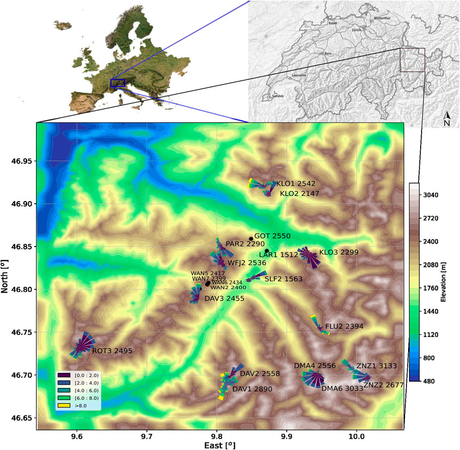
Figure 1. Map showing the domain of the 200 m resolution model and its location in the east of Switzerland. The black dots and wind roses give the locations of the stations with the name and elevation. The wind roses show the wind speed and direction of February - March 2019 measured by the corresponding station. Not all wind roses are shown as choice to not clutter the figure. The model topography is based on SRTM 1 arcsecond (National Geospatial-Intelligence Agency (NGA), 2000) and the map of Switzerland is acquired from SwissTopo (Swiss Federal Office of Topography, swisstopo, 2025).

2.1.1 Weissfluhjoch station

The WFJ station is located on a flatter section on a south-east facing slope at 2,536 m a.s.l. in the Parsenn ski area. Three peaks surround this field site: Weissfluhjoch (2,686 m a.s.l.) to the north, Salezerhorn (2,536 m a.s.l.) to the southeast, and Schafläger (2,681 m a.s.l.) to the southwest. On the research site, a Young RE-8500 sonic anemometer combined with a Li-COR 7500A gas analyzer is set up at a height of 3 m above snow-free ground. During the experiment, the effective height of the sensor varied between 95 cm and 0 cm above the snow surface, being partially buried in the snow on a few occasions. The measuring frequency of the sonic anemometer and the gas analyzer is 10 Hz. The research field site also contains an automatic weather station measuring temperature, wind speed, snow surface temperature, longwave radiation, and reflected shortwave radiation. These measurements are used for the computation of fluxes using the Monin-Obukhov bulk method (further discussed in Section 2.3.2).

The predominant wind directions at WFJ are either from the southeast or the northwest, which corresponds to up- and down-slope winds, respectively.

2.1.2 IMIS and wannengrat stations

The IMIS stations, operated by SLF, are situated at high-elevation locations to provide meteorological data for operational avalanche forecasts and warnings. There are thirteen IMIS stations located within the simulation domain of Figure 1. Ten of them are ‘snow’ stations and they provide snow depth, wind speed, air temperature, humidity, surface temperature, and reflected shortwave radiation, used as input for the surface model SNOWPACK. They are typically placed in more wind sheltered environments. The other three stations are ‘wind’ stations, typically placed on more wind exposed locations at a ridge. Here, they are only used for the comparison of air temperature, wind speed and relative humidity. More information on these stations can be found in Lehning et al. (1999).

Five additional automatic weather stations, which recorded data in February and March 2019, are located at the Wannengrat area, in Dischma valley and in Laret. Here, these stations are only used for air temperature, wind speed, relative humidity, and if available, surface temperature comparisons. For all stations, the wind speed is corrected to a height of 10 m using the logarithmic wind profile for comparison to the model results.

2.2 Event selection

To investigate the variability of turbulent fluxes depending on the synoptic flow, we selected three distinct weather patterns: a South Föhn, a North Föhn, and a calm day. Föhn is defined as a large-scale downslope wind induced by terrain characteristics that brings drier and warmer air to the lee side of the mountain range (Elvidge and Renfrew, 2016).

Davos, located in an inner valley on the north side of the main divide of the Alps, experiences different impacts depending on the direction of the föhn. During south föhn events, Davos is on the lee side, experiencing warm and dry descending air. In contrast, during north föhn events, the region is located more on the windward side, receiving moist, rising air often associated with precipitation. By comparing flux measurements during these föhn events to those recorded on a calm day, we aim to analyze the high-resolution spatial distribution of turbulent fluxes under varying meteorological conditions. Due to the high computational cost associated with running complex models at a 200 m resolution, we selected a single representative day for each event to simulate. The analysis is based on data from February and March 2019, a period characterized by a long dry spell in February and frequent precipitation events in March.

2.2.1 South föhn event

We define south föhn events in the months of February and March 2019 with an automatic detection with the following conditions at the WFJ site:

• constant wind direction from the south-west to south-east throughout the day,

• 30-min average wind speeds exceeding 5 m ${\text{s}}^{-1}$,

• low relative humidity (30%–60%),

• increasing 2 m air temperatures during the event.

Additionally, the maximum air temperature of the day should not exceed 0 °C at Weissfluhjoch as we want to avoid surface melting of snow, which may add further complexity to our conclusions. In these 2 months, 6 days are classified as south föhn events which we use in the analysis in Section 3.2. For the model simulation, we selected the sixth of March 2019. This day was characterized by a strong föhn event, and more than 80% of the sonic anemometer and gas analyzer data passed quality tests. On this day, the snow height at WFJ was 2.25 m, which means the sonic anemometer was 0.75 m above ground level. A rough flux footprint estimation based on Kljun et al. (2015) gives a maximum at 2.1 m.

2.2.2 North föhn event

For the automatic detection, north föhn events are defined based on the following conditions observed at the WFJ weather station:

• predominant wind direction from the north,

• 30-min average wind speeds exceeding 5 m ${\text{s}}^{-1}$,

• high relative humidity (close to 100%),

• decreasing 2 m air temperatures during the event.

Seven days in February and March 2019 met these criteria.

North föhn events are often accompanied by snowfall. Snow particles that pass through the sensor of the ultrasonic anemometer can influence the measurements by increasing the amount of spikes in wind and temperature values which makes the data unreliable (Sigmund et al., 2022). For the model simulation, we chose an event that was not accompanied by snowfall, as to have the largest amount of reliable EC data to compare with. One of the few days in February and March where a significant portion of the day showed reliable data from the sonic anemometer, was the 25th of March 2019. However, most of the gas analyzer data did not pass data quality control tests. Instead of obtaining latent heat flux from the high-frequency data, we computed the latent heat flux using the C-method, first introduced by Businger (1986) and revisited by González-Herrero et al. (2024). This method assumes that turbulent eddies transport heat and moisture in the same way, and thus the turbulent exchange coefficients for sensible and latent heat are equal $(C_l=C_s)$. Accordingly, the method requires only high-frequency measurements from the sonic anemometer, supplemented by low-frequency meteorological observations. The snow height at WFJ on this day was 2.6 m, corresponding to a sonic anemometer height of 0.4 m above the ground. A rough flux footprint estimation based on Kljun et al. (2015) gives a maximum at 2.0 m.

2.2.3 Calm event

To compare the synoptic flux-driven events to a day mainly driven by small turbulent fluxes, we selected calm days with wind speeds of less than 3 m ${\text{s}}^{-1}$ at the WFJ station. From the 20 days in February and March 2019 that met this criterion, we selected the 20th of February 2019 for the simulation. On this day, the Alps were under the influence of a high pressure zone, which resulted in quiescent wind in the study area. The snow depth at WFJ was 2.2 m, placing the sonic anemometer at an effective height of 0.8 m above the snow surface. A rough flux footprint estimation based on Kljun et al. (2015) gives a maximum at 1.6 m. A 2D flux footprint estimation for all three events is given in Supplementary Figure S1.

2.3 Data processing

2.3.1 Eddy covariance method

Before computing fluxes from high-frequency eddy covariance data, we applied a rigorous data pre-processing protocol. This included applying plausibility limits, despiking all high-frequency time series, correcting gas analyzer data, and performing a double rotation of the coordinate system. Turbulent fluxes were then calculated using the EddyPro software package (LI-COR, 2021). Data flagged as poor quality were excluded from further analysis. As a result of these quality control measures, only 57% of the data were retained for north föhn days, 75% for south föhn days, and 55% for calm days. A detailed description of the processing steps is provided in the Supplementary Material 1.

2.3.2 Monin-Obukhov parametrization

At the IMIS stations, as only low frequency data is available, we compute turbulent fluxes using the Monin-Obukhov Similarity Theory (MOST). For this we use the physics-based model SNOWPACK (Lehning et al., 2002). We force this model with snow depth, air temperature, wind speed, relative humidity, and reflected shortwave radiation. The SNOWPACK model, described in more detail below, solves the following equations for sensible ($Q_s$, W ${\text{m}}^{-2}$) and latent heat flux ($Q_l$, W ${\text{m}}^{-2}$), with Equations 1, 2, respectively:

$Q_s=-C_s\bar{U}{\rho }_a{c}_p\left(T_z-T_s\right),C_s=\frac{{\kappa }^2}{\left[ln\left(\frac{z}{z_0}\right)-{\varphi }_s\left(\zeta \right)\right]\left[ln\left(\frac{z}{z_0}\right)-{\varphi }_m\left(\zeta \right)\right]},(1)$

$Q_l=-C_l\bar{U}{\rho }_a{L}_s\left(q_z-q_s\right),C_l=\frac{{\kappa }^2}{\left[ln\left(\frac{z}{z_0}\right)-{\varphi }_q\left(\zeta \right)\right]\left[ln\left(\frac{z}{z_0}\right)-{\varphi }_m\left(\zeta \right)\right]},(2)$

where $\bar{U}$ is the mean wind speed (m ${\text{s}}^{-1}$), ${\rho }_a$ the air density (${\text{kgm}}^{-3}$), $c_p$ and $L_s$, the heat capacity and the latent heat of sublimation (${\text{Jkg}}^{-1}{\text{K}}^{-1}$ and ${\text{Jkg}}^{-1}$), respectively, $(T_z-T_s)$ and $(q_z-q_s)$ the temperature and humidity gradient between height $z$ and the surface, respectively, $\kappa$ the von Karman constant, and $z_0$ the roughness length (m). ${\varphi }_m,{\varphi }_s,{\varphi }_q$ are the stability functions for scalar quantities of momentum, sensible, and latent heat as a function of stability $\zeta$, which is dependent on the Richardson number (Foken, 2006).

CRYOWRF uses SNOWPACK as the land surface model (Sharma et al., 2021), therefore the offline SNOWPACK flux simulations are comparable to the ones from CRYOWRF. For the stability correction, we use the expressions of $\varphi$ by Holtslag and De Bruin (1988). This stability correction is one of the most widely used corrections and is recommended for very stable conditions (Andreas, 2002; Schlögl et al., 2017). The roughness length is set to $z_0=0.01$ m for all stations. This roughness length lies between the values computed by Judith and Doorschot (2004) for WFJ, and typical roughness lengths for snow (Clifton et al., 2006).

Roughness length computation from available high-frequency sonic anemometer data from WFJ resulted in similar values. For these computations, first a strong selection criteria for $u\ast$ is used to remove values of high $\frac{{\sigma }_w}{u\ast }$, which resulted in 635 measurements of $u\ast$ being used. Roughness length can be obtained in two ways. First by solving the logarithmic wind equation, which resulted in a roughness lengths of $z_0=0.032$ m. The second method, described by Panofsky (1984), considers integral turbulence characteristics, for which González-Herrero et al. (2024) argues that this yields better results. The computation of roughness length is done with Equation 3:

$z_0=z/exp\left(1.25\kappa \frac{\bar{U}}{{\sigma }_w}\right),(3)$

with ${\sigma }_w$ being the standard deviation of the horizontal wind velocity, $\bar{U}$ the mean wind horizontal wind velocity, and $\kappa$ the von Karman constant. This method yields $z_0=0.013$ m, which is about half the magnitude of values obtained from the logarithmic wind profile. As a trade-off between roughness lengths found by Judith and Doorschot (2004), (Clifton et al., 2006), and the two methods of roughness length calculation, we chose to use the roughness length of $z_0=0.01$ m for all stations.

2.4 Model setup

To estimate the spatial variability of the turbulent heat fluxes, we use the model CRYOWRF developed by the Snow and Avalanche Research Institute SLF and the EPFL Laboratory of Cryospheric Sciences. CRYOWRF couples the atmospheric model Weather Research and Forecasting (WRF) with the surface model SNOWPACK (Sharma et al., 2021). WRF is a widely used, non-hydrostatic, and fully compressible model. The model is resolved on Eulerian mass dynamic cores.

CRYOWRF is set up with a vertical grid of 65 layers on terrain-following hydrostatic-pressure coordinates, the first vertical grid point is set to $\sim$30 m and the domain extends up to 200 hPa. We use a total of 4 nested domains to run the model. The first domain has a resolution of 9 km and a total grid size of 1,080 km by 1,080 km. The following domains have a smaller domain size and a resolution of 3 km, 1 km, and 200 m, respectively. The computation timestep of the smallest domain is 0.06 s. For the output, data variables are averaged over 5-min intervals. The boundary conditions and the input for the first time step are extracted from ERA-5 Land with a resolution of 9 km, equal to the first domain. This domain has a spin-up time of 2 days. Sequentially, the next domains start with boundary conditions given by the previous domain, until the highest resolution domain starts 3 h prior to the day of interest. For the smallest domain, we use a topography resolution by STMR with 1 arcsecond (National Geospatial-Intelligence Agency NGA, 2000). A terrain smoothing option of 1-2-1 is applied 6 times, which is needed to smooth slopes over ${45}^o$. An example of a namelist. input file of a WRF run is given in the Supplementary Material 2.

WRF allows for a wide choice of physics and dynamics options, including several different land-surface models, planetary boundary layer (PBL) schemes, cloud microphysics schemes, and cumulus parameterizations. In this work, the PBL scheme is parametrized with the Yonsei University scheme (YSU) (Dudhia, 2010) for the first 3 domains, and domain 4 is run in Large Eddy Simulation (LES) mode. The YSU scheme is a first-order nonlocal scheme, with a countergradient term and an explicit entrainment term in the turbulence flux equation. Mixing terms are evaluated in physical space and the sub-grid-scale turbulence is solved by the horizontal Smagorinsky first-order closure. At the same time, the vertical diffusion is taken care of by the PBL scheme.

The surface model in CRYOWRF, SNOWPACK, is a one-dimensional model representing the snowpack at each grid point by a multi-layer column. SNOWPACK is able to merge snowpack layers if they are similar enough keeping the computational demand at a reasonable level. The model solves the heat equation, together with snow compaction and water percolation (Wever et al., 2014). WRF provides the surface meteorological variables to the snowpack part of the model every 5 min. SNOWPACK then calculates the sensible and latent fluxes, albedo and surface temperature which it then returns to WRF.

CRYOWRF additionally implements an blowing snow scheme as described by Sharma et al. (2021), which models the aeolian transport of snow particles, their sublimation, and re-deposition. The blowing snow model is a double-moment scheme that solves Eulerian advection-diffusion-type equations for the mass and number mixing ratios of blowing snow particles. This is done on an additional fine mesh grid between the surface layer and the first WRF layer. This scheme runs at every WRF timestep. The amount of snow eroded from the surface is computed by SNOWPACK based on the saltation mass flux from Sørensen (2004). The snow mass flux in saltation is then input into the lowest blowing snow fine mesh gridpoint for vertical advection.

3 Comparison between observed and modeled turbulent fluxes

3.1 Temporal variability of turbulent fluxes

The timeseries of turbulent fluxes during the three selected events of South Föhn, North Föhn, and a calm day in Figure 2 shows the temporal evolution of meteorological variables and sensible and latent heat fluxes derived from EC measurements. The South Föhn event is characterized by strong winds and enhanced turbulent exchange, with sensible heat flux directed towards the surface reaching values of up to −120 W ${\text{m}}^{-2}$. Latent heat fluxes during this event are also high, indicating substantial sublimation, up to 100 W ${\text{m}}^{-2}$. These increased sublimation magnitudes are consistent with reported fluxes under strong föhn conditions over snow (MacDonald et al., 2018; Francis et al., 2023).

Figure 2

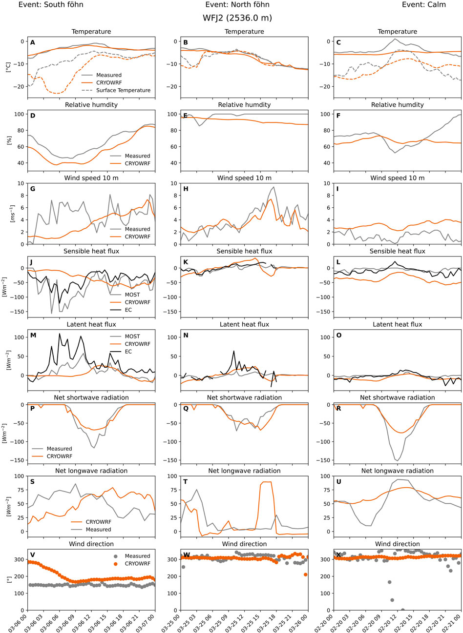
Figure 2. Measured and modeled variables for air and surface temperature (A–C) relative humidity (D–F) wind speed (G–I) sensible heat flux (J–L) latent heat flux (M–O) net shortwave radiation (P–R) net longwave radiation (S–U) and wind direction (V–X) for the WFJ station during three different events of a South Föhn (2019-03-06), North Föhn (2019-03-25), and a Calm day (2019-02-20). For the turbulent fluxes, both measurements from MOST and EC are given.

In contrast, during the North Föhn event the turbulent fluxes remain generally weaker. Sensible heat flux values are closer to zero and change between positive and negative values, reflecting reduced exchange compared to the South Föhn case. The latent heat flux shows lower sublimation estimates than during the South Föhn.

Under calm conditions, both sensible and latent heat fluxes are of low magnitude and display limited temporal variability and both fluxes show similar sign changes, positive during the day and negative at night. The weak turbulent exchange is consistent with stable near-surface stratification and reduced wind forcing.

3.2 MOST in complex terrain

Since MOST is widely used in numerical weather models such as CRYOWRF, we compare this method to the more direct EC technique for measuring turbulent fluxes and discuss the associated limitations. This allows us to estimate the source of errors from the computation method. From Figure 2, the panels J–O compare sensible and latent heat fluxes computed using EC and MOST, revealing that the two methods capture similar trends throughout the day. Sign changes in the fluxes are consistently captured by both methods, demonstrating agreement in the direction of the turbulent fluxes. However, the most notable differences lies in the magnitude of the latent heat fluxes, where EC shows a greater magnitude in general.

Combining multiple days classified as days with a south föhn, north föhn, or calm conditions (criteria described in Section 2.2), Figure 3 presents scatter plots of the 30-min averaged sensible and latent heat fluxes measured with EC against those computed using MOST. The correlation between the two methods varies considerably across weather events. For sensible heat flux, the highest correlation occurs during north föhn days, while the lowest is observed on calm days. For latent heat flux, the highest correlation occurs during south föhn days.

Figure 3

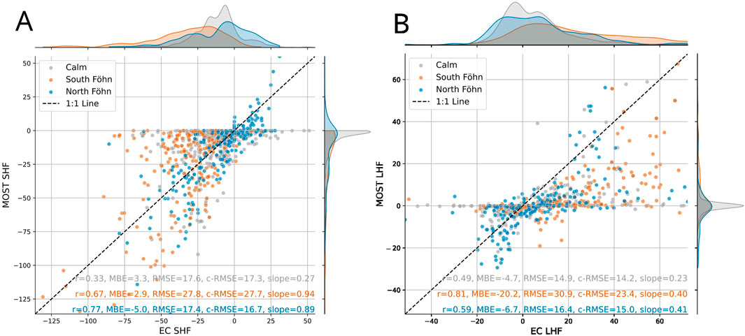
Figure 3. Scatter plot comparing MOST and EC 30-min averaged sensible heat flux (A) and latent heat flux (B) at the WFJ station. The colors show different events of days with a South Föhn, North Föhn, and calm days. The metrics show the correlation coefficient (r), mean bias error (MBE), root mean squared error (RMSE), centered root mean squared error (c-RMSE), and slope. The MBE values indicate a systematic underestimation of turbulent flux magnitudes by MOST. Note that for the North Föhn event, the MBE of the sensible-heat flux has the opposite sign compared with the other events, as both positive and negative flux values occur during this period.

The flux distributions for these events provide further insight into how each method captures variability. While MOST and EC yield similar overall ranges for both sensible and latent heat fluxes, their distributions differ markedly. MOST tends to produce a more normally distributed set of flux values, while EC captures a broader distribution, indicating greater variability. The Mean Bias Error (MBE) reveals that MOST generally underestimates turbulent flux magnitudes relative to EC. This bias arises because MOST values are more tightly clustered around the median, often closer to zero, whereas EC reflects a wider range of flux intensities.

Positive sensible heat fluxes over snow-covered surfaces are rare because surface temperatures usually do not exceed air temperatures. However, such cases can occur, particularly during cold air advection under cloudy conditions, which leads to rapid cooling of the air temperature while the surface experiences high incoming longwave radiation. This change of direction in the flux is only visible in north föhn events for both EC and MOST measurements.

During south föhn and calm conditions, when surface temperatures are lower than air temperatures, positive sensible heat fluxes observed in EC measurements can be a sign of advection. This advection is associated with the horizontal transport of heat and moisture, which is not directly driven by turbulence (Stiperski and Rotach, 2016). In these cases, the advection of warmer air leads to up- and downwards motions that disrupt the local energy balance, potentially contributing to the discrepancies observed in the sensible heat flux computed by EC compared to MOST.

Additionally, the low correlation and relatively high error during calm days can be partly attributed to the lack of quality of EC data. Calm conditions can lead to errors in aligning EC measurements with the double-rotated mean wind (Stiperski and Rotach, 2016), reducing accuracy. Additionally, during both north föhn and calm days, a significant portion of EC data fails quality control checks due to moisture in the sensors, leaving only a limited dataset for comparison (Sigmund et al., 2022).

We consider the main source of the observed differences between MOST and EC to be the limitations of applying MOST in complex terrain under stable conditions, where a constant-flux layer may not exist. The absence of such a layer means that the derived fluxes depend on the measurement height. Unfortunately, multiple EC levels were not available in our dataset to evaluate this effect directly. Schlögl et al. (2017), who analyzed two EC levels at the same WFJ site in 2007, showed that the constant-flux assumption (based on Stull, 1988) is valid only about 10% of the time at this location, resulting in height-dependent MBE. Our MBE for sensible heat flux agrees well with their reported underestimations of 2.3–5.9 W ${\text{m}}^{-2}$ when using the Holtslag stability functions. This consistency suggests that this parameterizations tends to over-suppress turbulent exchange under stable, snow-covered conditions.

Although both MOST and EC methods face limitations in complex terrain, MOST remains a valuable framework for understanding the drivers of variability in turbulent fluxes. This is because MOST explicitly relates flux magnitude to wind speed, temperature, and moisture gradients, quantities that are the drivers of the turbulent exchange.

3.3 Point comparison of CRYOWRF against measurements

Our findings confirm earlier studies that MOST does not always reproduce local EC measurements (Nadeau et al., 2013). However, we argue that MOST is still applicable as a flux parameterization in (larger scale) models since local fluxes are highly temporally variable while the model needs to represent the mean surface exchange successfully. Since we do not know the flux averaged over the grid cell of a model, we can only compare how well the mean quantities are reproduced by such a model. In this context, we evaluate the skill of CRYOWRF in reproducing measured values by comparing atmospheric and surface variables from CRYOWRF against those from 21 meteorological stations in the model domain. The quantities air temperature, humidity, wind and surface temperature are directly measured and turbulent fluxes are calculated using MOST. Figure 4 presents the mean absolute error (top number), correlation (bottom number), and bias (color) for key meteorological variables. These comparisons are conducted for the three simulations at two different resolutions: 1 km resolution, which is currently used in Swiss numerical weather prediction models, and at 200 m resolution, which is a very high resolution for such applications. Taylor plots showing the standard deviation, correlation and centered RMSE of both resolutions are shown in the Supplementary Figures S2, S3. The simulation resolution of 200 m is sufficient to resolve dominant length-scales of daily mean fluxes as shown in the mean daily flux semivariograms (Supplementary Figures S4, S5).

Figure 4

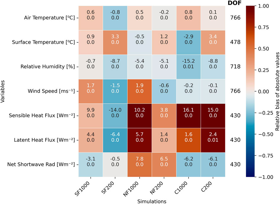
Figure 4. Mean Absolute Error (top number), correlation (bottom number), and relative bias of absolute values (color) of modeled compared to measured variables of air temperature, surface temperature, relative humidity, wind speed, sensible heat flux, latent heat flux, and shortwave radiation. The simulations represent the South Föhn, North Föhn and Calm day at resolutions of 1,000 and 200 m. The color of the squares gives the bias of model, with a red color indicating an overestimation and a blue color an underestimation in magnitude of the model. Overall, the higher resolution simulations show better metrics than coarser resolution simulations.

Overall, the higher resolution slightly improves correlations and reduces errors for variables such as air temperature, relative humidity, and wind speed, although it decreases the accuracy in surface temperature. For example, in the high-resolution simulation, the 2 m air temperature is well resolved across all events, with a correlation near 0.9, an MAE of less than 1.3 °C and a slight warm bias in air temperatures. However, the model shows a cold bias in surface temperatures, especially in the high-resolution simulation, leading to a higher temperature gradient between the surface and the air.

The model systematically underestimates relative humidity, particularly during the North Föhn event when moist air is advected from the north. At WFJ station, observations indicate near-saturated conditions (Figure 2 panels D–F), while the model fails to reproduce these, likely due to deficiencies in cloud representation–a known limitation in numerical weather prediction models (Otkin and Greenwald, 2008). This is evident in Figure 2, panel T, where the model simulates a spike in net longwave radiation, corresponding to a spurious clearing of clouds. This modeled clearing results in excessive surface cooling over a 3-h period, with net longwave losses reaching 100 W ${\text{m}}^{-2}$. Consequently, both the sensible and latent heat fluxes reverse sign—an effect not observed in either MOST or EC-derived fluxes. These errors in cloud representation impact the surface energy balance by altering incoming longwave and shortwave radiation, which in turn affects surface temperature and near-surface humidity, leading to wrong flux predictions.

Wind speed biases vary between resolutions. In the coarse-resolution simulation, wind speeds tend to be overestimated in the high wind scenarios, whereas in the high-resolution simulation, wind speeds are underestimated. This pattern holds across the entire domain, not just at individual station locations. For instance, during the South Föhn event, the mean wind speed in the coarse-resolution simulation is 6.0 m ${\text{s}}^{-1}$, while in the high-resolution simulation, it is only 2.7 m ${\text{s}}^{-1}$. We divided the stations into ‘wind’ and ‘sheltered’ categories and computed the relative bias for both resolutions, as shown in Figure 5. The coarser resolution captures wind velocities at ridge stations more accurately, whereas the higher resolution performs better at sheltered stations. This occurs because the simulated ridge–sheltered wind speed contrast is smaller than in the observations. On the calm day, this distinction disappears, as both simulations produce similar wind velocities due to the limited spatial variability in wind speed between sheltered and ridge locations. At coarser resolutions, the model smooths out complex topographic features such as ridges, valleys, and steep slopes. This leads to a less obstructed flow and, consequently, to higher modeled wind speeds in theoretically sheltered stations. In contrast, higher-resolution simulations capture finer-scale terrain features that induce flow blocking, stagnation, channeling, and turbulence, which act to reduce domain-wide wind speeds near the surface. As a result, the high-resolution simulation reflects more realistic wind interactions with terrain but may still underestimate wind speeds at ridges due to remaining unresolved features or due to misleading interpolation to station locations. Additionally, the choice of PBL scheme in the simulation contributes to wind speed differences. As studied by Zhang et al. (2021), no single PBL scheme universally outperforms others in complex terrain; rather, performance depends on specific meteorological conditions. Therefore, part of the wind speed bias in our simulations could be attributed to the PBL scheme employed.

Figure 5

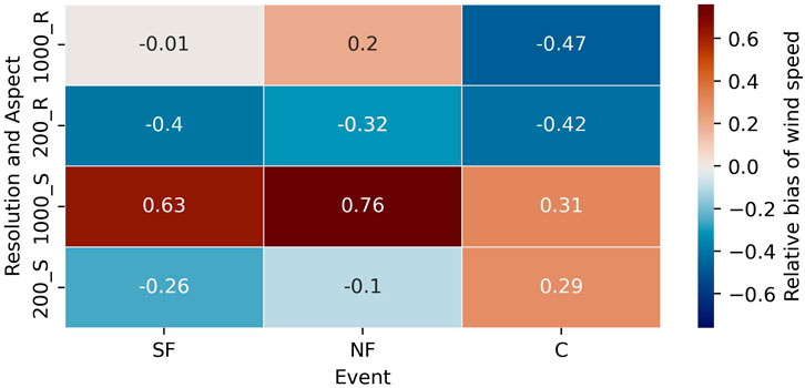
Figure 5. Relative bias of wind speed for stations located on ridges, noted by “_R″ and in sheltered locations, noted by “_S″ for all three events (SF, NF, and C) and both resolutions (200 m and 1,000 m). These metrics include 6 ridge stations and 13 sheltered stations. The 1,000 m resolution has higher wind velocities in general and represents better the ridge stations, whilst 200 m resolution represents better the sheltered stations wind lower wind velocities.

These wind biases directly translate into biases in turbulent fluxes predicted by MOST, leading to corresponding systematic errors. In turn, the underestimation of turbulent flux magnitudes in the high-resolution simulation may explain the increased surface temperature errors. A lower flux magnitude means less energy is transferred between the surface and the air, leading to stronger temperature gradients. However, this feedback takes time to develop. The South Föhn event at WFJ station exemplifies this effect, as seen in Figure 2. In the morning, the model overestimates the temperature gradient while underestimating wind speeds, resulting in lower fluxes than observed. Only later in the day does the turbulent flux magnitude increase, allowing the modeled surface temperature to match observed values.

When comparing daily mean turbulent fluxes from the WFJ station, the same station as shown in Figure 2, for EC, MOST, and model estimates, the variability in estimates is summarized in Table 1. In some cases, the model daily mean estimates align more closely with the EC means than MOST does, or the bias lies in the other direction. This suggests that, although errors in model input variables can strongly influence the results, the bias errors induced by MOST do not propagate linearly to model estimates and that the internal feedback processes in the model are effective in reproducing realistic fluxes. However, the latent heat flux does not show this compensation from feedback processes - and this shows a systematic bias from the MOST parameterizations.

Table 1

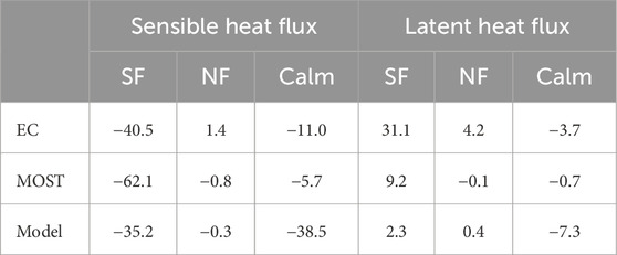
Table 1. Comparison of daily mean sensible and latent heat fluxes for the WFJ station computed with eddy covariance (EC), Monin-Obukhov (MOST), and model results for the three different events: South Föhn (SF), North Föhn (NF) and the Calm day in W ${\text{m}}^{-2}$. Gaps in EC data are filled by interpolating in time to obtain a daily mean.

In conclusion, the point comparisons highlight that higher model resolution generally improves the representation of meteorological variables such as air temperature, humidity, and wind speed. Systematic biases in wind and humidity are closely tied to terrain representation, cloud parameterizations, and the choice of PBL schemes. These biases propagate into the turbulent fluxes, which show low correlation with observations across events. Nevertheless, the time series suggests that fluxes can partially compensate for other model errors through feedback mechanisms.

4 Spatial and temporal variability of turbulent fluxes in CRYOWRF

4.1 Distribution of turbulent fluxes

Accepting the limitations in the model and keeping in mind the bias inferred from using MOST shown in the two previous sections, we can nonetheless use the model to investigate systematic spatial trends in turbulent fluxes based on the heterogeneity in the terrain which the model does resolve. To show the spatial variability within turbulent fluxes the histograms in Figure 6 illustrate the spatial range and average of daily mean turbulent flux values for the three different simulated cases across the domain. Among the three events, the South Föhn day exhibits the widest range and highest magnitudes of turbulent fluxes. The interquantile (25%–75%) range of sensible heat flux spans from −62 W ${\text{m}}^{-2}$ to −7 W ${\text{m}}^{-2}$, while the latent heat flux ranges from −1 W ${\text{m}}^{-2}$ to 16 W ${\text{m}}^{-2}$. During the North Föhn event, surface temperatures exceeded air temperatures in some locations, leading to some positive daily average values of sensible heat flux within the interquantile range of −15 W ${\text{m}}^{-2}$ and 1 W ${\text{m}}^{-2}$. The latent heat flux ranges from −3 W ${\text{m}}^{-2}$ to 7 W ${\text{m}}^{-2}$. On the calm day, the distribution of sensible heat fluxes falls between those of the two föhn events, with an interquantile range of −30 W ${\text{m}}^{-2}$ to −4 W ${\text{m}}^{-2}$. The latent heat flux distribution is shifted toward more negative values than the previous mentioned cases, ranging from −3 W ${\text{m}}^{-2}$ to 0 W ${\text{m}}^{-2}$.

Figure 6

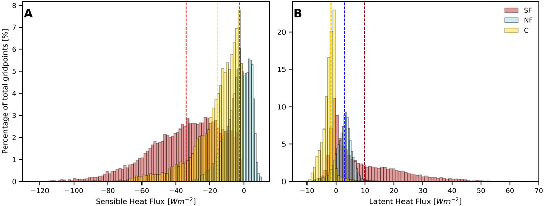
Figure 6. Distribution of spatial sensible (A) and latent (B) heat flux values averaged over a full day for each simulated case, South Föhn in red, North Föhn in blue and a Calm day in yellow. The dashed vertical lines show the mean value over all gridpoints.

For comparison, the domain-wide daily average of net shortwave radiation is 23 $\pm$ 7.7 W ${\text{m}}^{-2}$, 26 $\pm$ 8.1 W ${\text{m}}^{-2}$, and 23 $\pm$ 7.3 W ${\text{m}}^{-2}$ for the South Föhn, North Föhn, and calm day, respectively. Notably, on the South Föhn day, the daily average energy supplied to the surface by sensible heat flux exceeds that of net shortwave radiation. This highlights that an accurate representation of turbulent fluxes over snow-covered terrain is crucial, especially during midwinter when albedo is high and the sun angle is low, as they can contribute significantly to the energy exchange between the air and the snowpack.

4.2 Temporal evolution of wind and resulting flux patterns

In complex terrain, wind patterns typically follow a diurnal cycle during fair weather, driven by thermal processes (Zardi and Whiteman, 2012). These thermal wind systems are most pronounced under clear sky conditions when synoptic winds are weak. However, when synoptic winds strengthen, dynamically-forced terrain flows become more dominant (Whiteman, 2000). To examine the spatial distribution of turbulent fluxes, Figure 7 presents the sensible and latent heat fluxes, for three different times of each event. During the South Föhn event, the highest turbulent flux magnitudes are observed along ridges perpendicular to the synoptic wind and in valleys where the synoptic wind aligns with thermal flows. The wind velocities intensify throughout the day, resulting in stronger sensible heat fluxes following the same spatial trends. Valleys exhibit particularly strong turbulent flux magnitudes as wind velocities increase due to thermally driven flows. In general, sublimation dominates at midday and at lower elevations in the afternoon, whereas deposition is more frequent in the morning and at elevations above 2,700 m. However, this trend is not entirely uniform over the elevations.

Figure 7

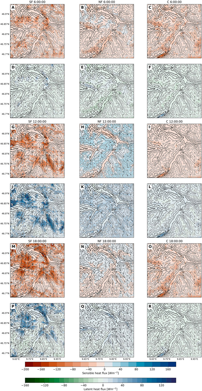
Figure 7. Maps with hourly averaged sensible heat flux (A–C,G–I,M–O) and latent heat flux (D–F,J–L,P–R) for the South Föhn (SF) (A,D,G,J,M,P) North Föhn (NF) (B,E,H,K,N,Q) and Calm day (C) (C,F,I,L,O,R) in the morning at 6:00, midday at 12:00 and afternoon 18:00. The black arrows show the velocity and direction of the wind in that hour. The contours show the topography, with lighter grey colors being higher elevations. The displayed domain corresponds to Figure 1 but with trimmed borders to minimize boundary effects. Clear variations between the events are evident: during the South Föhn, turbulent flux magnitudes increase throughout the day; during the North Föhn, fluxes change sign between midday and morning/afternoon; and during the Calm event, variations remain comparatively weak.

Unlike the South Föhn event, the North Föhn event exhibits markedly different spatial distributions throughout the day. In the morning, sensible and latent heat fluxes are predominantly negative across the domain, with some positive values in high elevation areas in the northern regions. The strongest fluxes occur on ridges, where wind velocities are high, and on south-facing slopes, where the synoptic flow aligns with downslope thermal winds, leading to descending dry air. In the midday, the pattern shifts: below approximately 1900 m, sensible heat flux remains mostly negative, whereas at higher elevations, it turns positive. Latent heat flux indicates widespread sublimation across the domain, with generally higher magnitudes at higher elevations. Notably, while elevation has little influence on turbulent fluxes in the morning, it becomes a key factor during the midday.

On the calm day, there are no substantial differences between morning and afternoon turbulent flux distributions. The wind remains predominantly from the north but is weak, allowing local thermal downslope flows to override the synoptic wind in certain areas. Similar to the North Föhn day, wind velocities are highest at ridges and south facing slopes, creating highest turbulent flux magnitudes at those wind prone locations. During midday wind velocities are particularly low, there is little turbulent exchange between the surface and the air, and only lower elevations are subject to some sublimation.

The cross-sections presented in the electronic Supplementary Material S10-12 illustrate the variability in wind velocity, where the key drivers of these fluctuations—thermally and dynamically-forced wind patterns—can be identified. The animations of potential temperature with cloud fraction and wind velocity illustrate the spatio-temporal variability of potential temperature, wind velocity, turbulent kinetic energy, and turbulent fluxes of sensible and latent heat through multiple cross-sections:

• CS2: Cross-section through two side valleys—Sertig (southwest valley) and Dischma (northeast valley) — that slope downward towards the main Landwasser valley

• CS6: North-South cross-section at 9.85°E spanning the entire domain

The wind velocity field generally aligns with the synoptic wind direction; however, local topography significantly modifies the flow. Orographic features create distinct wind patterns, including cross-ridge flows with crest speedups and recirculation zones characterized by reduced wind speeds on leeward slopes. Cross-ridge flows have been extensively studied by Lewis et al. (2008), who used automatic weather station measurements within our simulation domain near the Gaudergrat ridge, which has a typical length scale of L = 500 m. Raderschall et al. (2008) modeled these flow features using very high horizontal and vertical resolution of 25 m and $\sim$3 m in the lowest atmospheric layers, respectively. Despite the coarser resolution of our simulations, we still capture crest speed-ups near prominent ridges. One clear example is Gotschnagrat (CS6 SOUTH 19:00, 46.85 °N), where we observe a distinct acceleration of wind near the ridge crest. This localized increase in wind speed enhances turbulent energy exchange, resulting in an increase of sensible heat flux by approximately 25 W ${\text{m}}^{-2}$ and latent heat flux by 18 W ${\text{m}}^{-2}$ per 100 m of horizontal distance.

During the South Föhn event, both thermally and mechanically driven flows strongly influence wind velocity in addition to the synoptic flow, thereby affecting turbulent fluxes. Notable phenomena include gravity waves, thermally driven downslope and valley flows, the formation of cold-air pools, and their subsequent erosion.

The thermally driven downslope flows observed in the cross-valley (CS2) sections are particularly pronounced after 20:00 h, resulting in the onset of strong wind velocities in the Sertig valley (9.84 °E). A characteristic katabatic jet manifests within the valley core, where wind speeds reach up to 12 m ${\text{s}}^{-1}$. This downslope flow facilitates significant energy exchanges, formed by pronounced temperature gradient prevalent in low-elevation valleys coupled with high wind velocities, as indicated by substantial sensible heat fluxes of −200 W ${\text{m}}^{-2}$ and latent heat flux of 100 W ${\text{m}}^{-2}$. Katabatic flows exhibit a distinct vertical structure characterized by variations of turbulent fluxes with height. Specifically, negative momentum fluxes are typically present below the wind speed maximum and positive momentum flux above (Grachev et al., 2016). However, the vertical resolution of our simulation is insufficient to capture this near-surface dynamics.

In animation CS6, undulations in the potential temperature and wind fields—propagating from south to north between 06:00 and 24:00—indicate the presence of mountain-induced atmospheric gravity waves. These waves are most pronounced when the boundary layer is highly stable, such as those observed during the South Föhn event. The animation further reveals that wave troughs, where descending motions reach the surface, coincide with regions of higher surface wind speeds (e.g., at 46.75 °N at 12:00). These regions exhibit intensified and intermittent turbulence primarily driven by shear-induced mechanical mixing and turbulent kinetic energy dissipation, as the wave trough passes. Vosper et al. (2018) highlight the important role of gravity waves in modulating surface exchange and emphasize the challenges of capturing these effects in kilometer-scale NWP models. Kristianti et al. (2024) previously investigated the impact of mountain wave activity on wind power production in Switzerland, focusing on turbine heights of approximately 100 m using the high-resolution COSMO-WRF model. Their findings demonstrated an influence of mountain waves on wind production at these heights. In our simulations, we observe that the effects of mountain gravity waves extend all the way to the surface, impacting near-ground turbulent fluxes and exchange processes.

The valley between Landquart and Klosters (46.89 °N), located north of Davos, contains a stably stratified cold-air-pool (CAP) during the day, visible in CS6. When there are strong CAPs, the air within the CAP is decoupled from the overlying air, which causes weak winds in the valley, and turbulence is also weak (Mahrt, 1999; Gonzalez et al., 2019). Above the CAP, the advected air by the föhn induces strong shear-induced turbulence, which can be seen by the high turbulent kinetic energy above the CAP. The Richardson number is below 0.25 at this location. When the wind shear strengthens at the end of the day, it erodes the CAP, creating high turbulent fluxes in the valley.

During the North Föhn day, thermally driven flows are less pronounced. Unlike the South Föhn event, surface cooling in the evening is weaker due to the presence of a cloud cover and the associated increased incoming longwave radiation. As a result, the temperature gradient between the surface and the air is reduced, limiting the development of thermally driven flows. Consequently, the synoptic flow dominates, primarily governing wind velocity and direction. The spatial distribution of turbulent flux magnitudes thus coincide with dynamically-forced terrain flows.

Past studies have shown the importance of the contribution of drifting and blowing snow to total sublimation, which is defined as the sum of surface sublimation and sublimation from blowing snow particles. For example, Vionnet et al. (2014) simulated a case at Col du Lac Blanc in the French Alps and found that including blowing snow increased total sublimation by a factor of three. Similarly, Strasser et al. (2008) emphasized the importance of accounting for blowing snow sublimation in snow mass balance studies. In contrast, Groot Zwaaftink et al. (2013) found that while blowing snow sublimation can be significant on short timescales and in specific locations, its contribution is minor when averaged over a season. Their study, conducted in the 2.4 km² Wannengrat area (within our study domain), reported only a small seasonal contribution of drifting snow sublimation.

We analyzed sublimation in our CRYOWRF simulations, distinguishing between surface and blowing snow contributions. Figures showing accumulated surface and blowing snow sublimation have been added in Supplementary Material S6, S7. Our results show that, for the selected events, sublimation from blowing snow is localized and generally small. When averaged over the domain, surface sublimation dominates and is approximately an order of magnitude greater than sublimation from blowing snow in the North Föhn event and much smaller in the South Föhn event where surface sublimation values are significantly larger. These findings suggest that, while drifting snow sublimation may be important locally and during selected events, it does not significantly impact overall mass balance rates.

4.3 Terrain features driving spatial variability

The previous section showed how the wind field, both thermally and synoptically driven, shape the turbulent flux distribution. Other drivers of turbulent flux magnitude are the temperature and humidity gradients between the surface and the overlying air. During melting events, when surface temperatures remain constant at 0 °C, these gradients are governed by atmospheric properties. Pohl et al. (2006) conducted a study of the spatial variability of turbulent fluxes over melting snow in complex terrain with a simple model. In their case, they only varied the turbulent heat fluxes due to wind differences throughout the domain. In our cases, both surface and atmospheric properties play a significant role. Terrain features such as slope angle, aspect, and elevation shape both the wind field and these gradients, thereby influencing turbulent flux variability. The spatial distribution maps in Figure 7 suggest that both elevation and aspect contribute to the magnitude of turbulent fluxes. Here we attempt to quantify the extent to which this variability is driven by local wind velocities versus other terrain-induced factors.

Figure 8 presents plots of turbulent heat flux versus wind speed, categorized by elevation averaged over 12 h in the afternoon. This time division is chosen as during both wind-driven events the wind velocities associated with föhn winds peak during the afternoon. Consequently, turbulent fluxes reach higher magnitudes in the afternoon compared to the morning for the föhn cases.

Figure 8

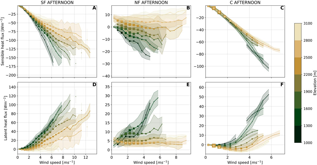
Figure 8. Sensible (A–C) and latent (D–F) heat flux against wind speed per elevation bin for each event in the afternoon 12-00. The squares give the sensible heat flux mean per 0.5 m ${\text{s}}^{-1}$ wind speed bin per elevation bin. The size of the square gives the relative amount of gridpoints in that elevation and wind speed bin. The shaded area contains 70% of the data in that bin, with a range from the 15th to 85th percentile.

Examining the elevation-dependent plots reveals a distinct variation in trends across elevation bins. In some cases the wind and flux magnitude scale linearly, for example, in the South Föhn afternoon the r-values range between −0.80 and −0.97, p-values $<$ 0.001. In other cases, such as the Calm afternoon, the curves display different functional forms but remain broadly consistent across elevations. Overall, at lower elevations, the magnitude of sensible heat flux increases more rapidly with increasing wind speeds compared to higher elevations. A similar pattern is observed for latent heat flux, though with opposite sign and a different curve shape. This pattern is less clear in the morning (not shown), when wind velocities are lower, as the higher wind velocities enhance differences in gradients between elevation in the turbulent flux magnitudes. Plots showing a breakdown by slope aspect and angle showed less variability (not shown), as the effect of elevation dominates over the effect of aspect at this resolution.

Figure 9 illustrates the temperature and water vapor mixing ratio gradients between the surface and the air at 2 m during the afternoon across different elevations. While elevation influences these gradients, wind velocity plays a dominant role in that higher wind speeds enhance turbulent mixing, thereby reducing temperature and moisture gradients. Air temperature is not influenced by wind velocity and shows a nearly perfect negative correlation with elevation, with correlation coefficients of −0.99 and −0.98. The lapse rate follows 7.2 °${\text{C km}}^{-1}$ for the South and North Föhn events, and 6.8 °${\text{C km}}^{-1}$ for the calm day, the latter being close to the moist adiabatic lapse rate. In contrast, surface temperature is controlled by wind velocity. Higher wind speeds reduce temperature gradients by enhancing turbulent mixing, which facilitates heat exchange between the surface and the atmosphere.

Figure 9

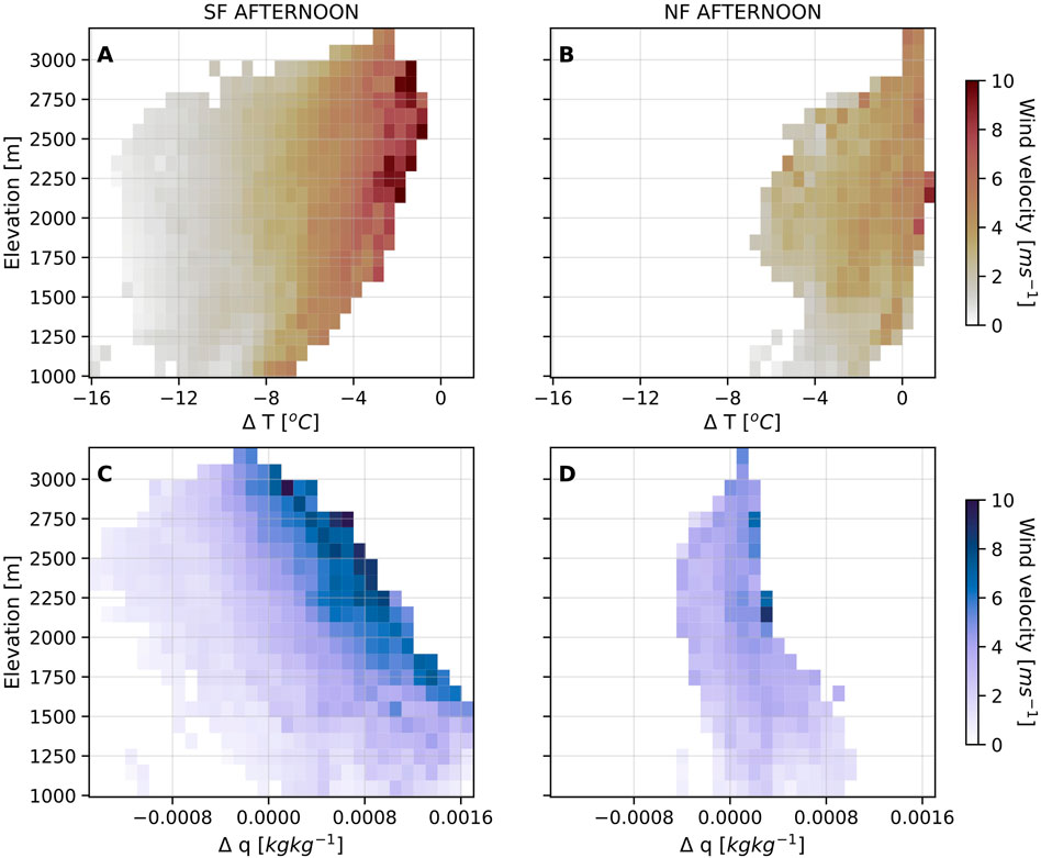
Figure 9. Temperature gradient (A,B) and water vapor mixing ratio gradient (C,D) between the surface and 2 m height for the South Föhn day and the North Föhn day in the afternoon from 12:00 to 00:00 throughout elevations. The color indicates the mean wind velocity magnitude at each elevation and gradient.

Differences in temperature gradients between south- and north-facing slopes are often attributed to variations in solar radiation. For example, a study by Robledano et al. (2021) at Col du Lautaret, France, using the 10 m resolution Rough-SEB model, demonstrated that topography, and in particular aspect, was the primary driver of surface temperature variations due to differential shortwave radiation exposure. In contrast, our simulations suggest that at our coarser resolution, aspect does not contribute as significantly to surface temperature variability. Instead, wind velocity plays a more dominant role, primarily through the feedback with turbulent fluxes. Slope aspects experiencing higher mean wind speeds exhibit enhanced surface-air mixing, which leads to lower temperature gradients. This pattern is evident in our results, shown in Supplementary Figures S8, S9 in the Supplementary Material.

On the South Föhn day, the water vapor mixing ratio gradient is primarily dictated by surface temperature. Since the water vapor content of the air remains relatively uniform across the domain, independent of air temperature, spatial variability in the gradient is driven by differences in surface temperature. In contrast, on the North Föhn day, air at higher elevations reaches relative humidity values close to 100%, causing the water vapor gradient to follow the air temperature gradient. At lower elevations, where the air is not fully saturated, air water vapor content is higher than at the surface leading to sublimation. The near-saturation of high elevation compared to lower saturation values at low elevation is typical for synoptic wind patterns which drive orographic precipitation, as discussed in Houze Jr (2012).

Although temperature and humidity gradients generally decrease with elevation—leading to a reduced potential for turbulent exchange at a given wind speed—the combined sensible and latent heat fluxes actually increase in magnitude with elevation due to stronger wind velocities, as shown in Figure 10. During both the South Föhn event and the calm day, this results in an increase in energy directed towards the snowpack with elevation, which promotes lateral energy transfer from higher to lower elevations. In contrast, during the North Föhn event, turbulent fluxes act to extract energy from the surface, with their magnitude intensifying at higher elevations. These differences throughout elevations are most pronounced when both föhn events are at their peaks in the afternoon. This highlights the dominant role of terrain features, such as elevation, driving the energy balance. Additionally, it shows that wind speed magnitudes are a stronger driver of the net turbulent flux than temperature and humidity gradients magnitudes, as the gradients decrease through the feedback with turbulent fluxes.

Figure 10

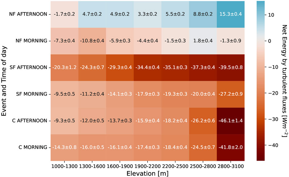
Figure 10. Sum of the sensible and latent heat fluxes and the 95% bootstrap confidence interval averaged over the morning (00:00-12:00) and the afternoon (12:00-00:00) per elevation range of bins of 300 m in W ${\text{m}}^{-2}$. The table shows a general trend of a monotonic increase in net turbulent flux with increasing elevation.

5 Discussion and conclusion

Turbulent heat fluxes play a crucial role in snow-covered environments, driving surface exchange processes that regulate snow energy balance. However, their spatiotemporal variability, particularly in complex terrain, remains insufficiently studied. Given the limited availability of direct heat flux measurements, we addressed this gap through a modeling approach. Since most numerical weather prediction models rely on flux-gradient similarity theories to estimate turbulent fluxes, which are often debated in complex terrain, we first compared the MOST prediction to EC measurements for the well-equipped WFJ site. Although both approaches generally align in terms of overall trends and flux direction, MOST underestimates flux magnitudes compared to EC measurements. This is in line with estimations from Schlögl et al. (2017) which reveal underestimations of sensible heat flux magnitude at the WFJ site between 2.3 and 5.9 W ${\text{m}}^{-2}$ with the Holtslag parametrization depending on measurement height. Our underestimation is most pronounced for latent heat fluxes, with underestimations of MBE reaching up to 20 W ${\text{m}}^{-2}$. Such systematic underestimation highlights the limitations of MOST in representing the full range of observed variability, despite its widespread application in NWP models, a finding consistent with previous studies (Sigmund et al., 2022; Nadeau et al., 2013; Stiperski and Calaf, 2023). Because MOST underestimates latent heat flux magnitudes by 4.7–20.2 W ${\text{m}}^{-2}$ and sensible heat flux by 2.9–3.3 W ${\text{m}}^{-2}$ in stable conditions, all subsequent model-based latent heat flux fields should be regarded as lower-bound estimates.

However, the comparison of daily mean turbulent fluxes from EC, MOST, and model estimates demonstrates that internal feedbacks within CRYOWRF play a key role in moderating bias propagation. While biases in the input variables or in the MOST parameterization affect individual flux components, these errors do not translate linearly into the modeled fluxes. Instead, the coupled interactions between wind speed, temperature gradients, and the surface energy balance tend to compensate for part of the imposed bias, allowing the model to reproduce more realistic daily mean fluxes. Consequently, the turbulent flux errors interact with and are partially dampened by adjustments in the mean meteorological fields, illustrating the self-regulating nature of the model’s feedback processes.

We proceed to compare CRYOWRF predictions over complex terrain of mean quantities and turbulent fluxes to values measured at 21 meteorological stations. Even though we have shown that the simulations with CRYOWRF over complex terrain was able to represent average surface exchange and therefore could produce useful estimates of mean quantities such as air and surface temperature or humidity, our findings indicate that accurately capturing dynamics at a single point in complex terrain remains challenging. When increasing the model resolution from 1 km to 200 m we see improvements in correctly representing most variables. But even the 200 m resolution, while high, is insufficient to replicate point measurements accurately. Wind speed discrepancies across model resolutions significantly influence the accuracy of turbulent flux predictions. For instance, 1 km resolution—a typical resolution for NWP models Kruyt et al. (2018) —leads to wind speed overestimations, especially at sheltered stations, while 200 m resolution tends to underestimate wind speeds, especially at stations on ridges. Consequently, inaccuracies in wind fields are the primary source of error in model-predicted turbulent fluxes, as underestimated wind velocities result in incorrect flux calculations. This, in turn, underestimates surface temperatures through a feedback from turbulent fluxes.

Although some variables are well resolved in CRYOWRF, limitations remain when applying state-of-the-art models to complex, snow-covered terrain. One constraint is the smoothing of steep slopes to prevent numerical instabilities, which reduces topographic realism. This smoothing also prevents the model from capturing small-scale terrain features such as hills or subtle convex and concave slopes- elements which can diverge wind fields or produce shading. This omission can lead to discrepancies between model output and observations, particularly in the variables of wind velocities and incoming shortwave radiation, which in turn propagate through to surface temperature and turbulent flux predictions. Additionally, the model assumes a uniform snow cover due to the coarse resolution of input data, neglecting the patchy distribution often observed at lower elevations. Patchy snow cover can substantially alter boundary layer dynamics, as extensively studied by Mott et al. (2015); Haugeneder et al. (2024a), Haugeneder et al. (2024b).

Another potential source of variability is the roughness length, which we assumed to be spatially constant over snow-covered pixels in the simulations. This simplification removes real-world variations. A previous study over East Antarctica by Amory et al. (2017) highlight that roughness length temporally varies over snow as sastrugi form. We assume, however, that the consequences on turbulent fluxes are limited as feedback effects, such as higher roughness length reducing wind speeds and consequently lowering turbulent fluxes, are potentially present. Yet, the exact impact of this interaction within the model remains uncertain. Further investigations are required to quantify these effects.

Despite these limitations, our simulations provide a first quantitative assessment of the spatial variability of turbulent fluxes over complex, snow-covered terrain using CRYOWRF. Although the terrain representation is slightly idealized due to slope smoothing and the assumption of a uniform snow surface, the results nevertheless offer valuable insights into the underlying processes governing surface–atmosphere exchange. To examine the impact of different synoptic weather patterns we focus on the spatial and temporal variability of turbulent fluxes during a south and North Föhn day, comparing them to a day without a predominant synoptic influence. The findings reveal substantial differences in both the range and spatial distribution of turbulent fluxes between these events, with the stable South Föhn event contributing significantly to energy transfer to the surface.

Other studies investigating the spatial variability of turbulent fluxes Pohl et al. (2006) or specifically sublimation Stigter et al. (2018) have highlighted the importance of wind fields in shaping spatial flux patterns. Our analysis the key role of wind fields in shaping both temporal and spatial variability of turbulent fluxes. In our case studies, wind velocities are influenced by a combination of synoptic forcing, local topography, and thermal effects. In contrast to the above-mentioned studies, our simulation does not use prescribed meteorological variables to drive the flux estimates. Instead, the model explicitly accounts for feedbacks of the computed turbulent fluxes on atmospheric and surface variables.

When examining the effects of different terrain features on mean turbulent flux magnitudes, excluding variations that arise from wind velocity, we find that elevation induces the most variability. This establishes a consistent relationship between wind speed and turbulent flux, where similar elevations exhibit comparable flux responses under similar wind conditions. Higher elevations are generally subject to lower humidity and temperature gradients, which result in lower magnitude flux for a given wind speed than lower elevation. This relationship is most pronounced when wind velocities are high, such as during the peak hours of the föhn events in the afternoon. Despite this, higher elevations still contribute more to heat extraction from the atmosphere over the snow-covered mountain terrain during both South Föhn and calm days, primarily due to the stronger wind speeds at these elevations. Conversely, during the North Föhn day, this pattern reverses and higher elevations exhibit greater heat loss from the surface to the atmosphere. Due to budgetary constraints, research on turbulent heat fluxes in complex terrain, aimed to understand snow melt or mountain boundary layer exchange, typically rely on data from only one or a few stations Litt et al. (2017); Reba et al. (2012); Cullen et al. (2007). Our results indicate the limited possibility of extending the turbulent flux estimates to areas subject to different wind velocities or at different elevations.

Given these findings, accurately resolving wind fields is the most important feature for correctly resolving the turbulent fluxes in NWP models. As demonstrated in this study, higher-resolution models offer slight improvements in wind field representation, which in turn improves the simulation of energy and mass transfer between the snowpack and the surface. This indicates that future computational capacity to compute operational high-resolution simulations will become a key factor for accurate real-time mass and energy balance estimates. Because wind fields directly influence the magnitude of turbulent fluxes, they also play a key role in regulating the temperature gradient between the surface and the air through enhanced mixing. This effect is particularly important at high elevations in midwinter, where radiative heating is limited by low solar angles and high albedo given the uniform snow cover. Under these conditions, turbulent fluxes can contribute more energy to the surface than solar radiation, with sensible heat flux even reaching double the magnitude of net solar radiation on a South Föhn day, making their accurate representation in models even more critical.

Data availability statement

Publicly available datasets were analyzed in this study. This data can be found here: The code of CRYOWRF is publicly available on gitlab at https://gitlabext.wsl.ch/atmospheric-models/CRYOWRF (v1.1). An example of the namelist. input file used for the simulation can be found in the Supplementary Material. ERA5-Land hourly reanalysis data was used to run the model and is publicly available on https://cds.climate.copernicus.eu/datasets/reanalysis-era5-pressure-levels. Meteorological data of all stations used in this study will be soon publicly available in a dataset paper in preparation by Bavay et al. and IMIS station data can be found directly on https://measurement-data.slf.ch/.

Author contributions

RE: Validation, Writing – review and editing, Investigation, Formal Analysis, Visualization, Writing – original draft, Methodology. SG-H: Conceptualization, Supervision, Writing – review and editing, Investigation. FG: Software, Investigation, Writing – review and editing. NW: Investigation, Writing – review and editing, Software. ML: Funding acquisition, Writing – review and editing, Supervision, Investigation, Conceptualization.

Funding

The author(s) declare that financial support was received for the research and/or publication of this article. The work was funded by the Swiss National Science Foundation (Project: Large-Scale Influence of Small-Scale Snow Processes; SNF-Grant: 215406), and the Swiss National Supercomputing Centre (CSCS) projects s1115, s1242, s1308.

Acknowledgements

We thank Mathias Bavay for his support in preparing and maintaining the meteorological station datasets used in this study. His efforts ensured the availability and quality of the observational data.

Conflict of interest

The authors declare that the research was conducted in the absence of any commercial or financial relationships that could be construed as a potential conflict of interest.

The handling editor MMF declared a past co-authorship with the authors NW, ML.

The author(s) declared that they were an editorial board member of Frontiers, at the time of submission. This had no impact on the peer review process and the final decision.

Generative AI statement

The author(s) declare that Generative AI was used in the creation of this manuscript. Generative AI technology (ChatGPT, GPT-4, OpenAI) was used to assist in editing and refining portions of the manuscript. All AI-generated content was thoroughly reviewed and edited by the authors to ensure accuracy and integrity.

Any alternative text (alt text) provided alongside figures in this article has been generated by Frontiers with the support of artificial intelligence and reasonable efforts have been made to ensure accuracy, including review by the authors wherever possible. If you identify any issues, please contact us.

Publisher’s note

All claims expressed in this article are solely those of the authors and do not necessarily represent those of their affiliated organizations, or those of the publisher, the editors and the reviewers. Any product that may be evaluated in this article, or claim that may be made by its manufacturer, is not guaranteed or endorsed by the publisher.

Supplementary material

The Supplementary Material for this article can be found online at: https://www.frontiersin.org/articles/10.3389/feart.2025.1640842/full#supplementary-material

References

Amory, C., Gallée, H., Naaim-Bouvet, F., Favier, V., Vignon, E., Picard, G., et al. (2017). Seasonal variations in drag coefficient over a sastrugi-covered snowfield in coastal east Antarctica. Boundary-Layer Meteorol. 164, 107–133. doi:10.1007/s10546-017-0242-5

CrossRef Full Text | Google Scholar

Andreas, E. L. (2002). Parameterizing scalar transfer over snow and ice: a review. J. Hydrometeorol. 3, 417–432. doi:10.1175/1525-7541(2002)003<0417:pstosa>2.0.co;2

CrossRef Full Text | Google Scholar

Businger, J. (1986). Evaluation of the accuracy with which dry deposition can be measured with current micrometeorological techniques. J. Appl. Meteorology Climatol. 25, 1100–1124. doi:10.1175/1520-0450(1986)025<1100:eotaww>2.0.co;2

CrossRef Full Text | Google Scholar

Clifton, A., Rüedi, J.-D., and Lehning, M. (2006). Snow saltation threshold measurements in a drifting-snow wind tunnel. J. Glaciol. 52, 585–596. doi:10.3189/172756506781828430

CrossRef Full Text | Google Scholar

Cullen, N. J., Mölg, T., Kaser, G., Steffen, K., and Hardy, D. R. (2007). Energy-balance model validation on the top of Kilimanjaro, Tanzania, using eddy covariance data. Ann. Glaciol. 46, 227–233. doi:10.3189/172756407782871224

CrossRef Full Text | Google Scholar

Dudhia, J. (2010). Wrf physics options. NCAR WRF basic Tutor. 26, 30.

Google Scholar

Elvidge, A. D., and Renfrew, I. A. (2016). The causes of foehn warming in the lee of Mountains. Bull. Am. Meteorological Soc. 97, 455–466. doi:10.1175/bams-d-14-00194.1

CrossRef Full Text | Google Scholar

Epifanio, C. C. (2007). A method for imposing surface stress and heat flux conditions in finite-difference models with steep terrain. Mon. weather Rev. 135, 906–917. doi:10.1175/mwr3297.1

CrossRef Full Text | Google Scholar

Foken, T. (2006). 50 years of the monin–obukhov similarity theory. Boundary-Layer Meteorol. 119, 431–447. doi:10.1007/s10546-006-9048-6

CrossRef Full Text | Google Scholar

Francis, D., Fonseca, R., Mattingly, K. S., Lhermitte, S., and Walker, C. (2023). Foehn winds at pine island glacier and their role in ice changes. Cryosphere Discuss. 2023, 3041–3062. doi:10.5194/tc-17-3041-2023

CrossRef Full Text | Google Scholar

Gadde, S., and van de Berg, W. J. (2024). Contribution of blowing-snow sublimation to the surface mass balance of Antarctica. Cryosphere 18, 4933–4953. doi:10.5194/tc-18-4933-2024

CrossRef Full Text | Google Scholar

Goger, B., Rotach, M. W., Gohm, A., Stiperski, I., and Fuhrer, O. (2016). “Current challenges for numerical weather prediction in complex terrain: topography representation and parameterizations,” in 2016 international conference on high performance computing and simulation (HPCS) (IEEE), 890–894.

CrossRef Full Text | Google Scholar

Goger, B., Stiperski, I., Nicholson, L., and Sauter, T. (2022). Large-eddy simulations of the atmospheric boundary layer over an alpine glacier: impact of synoptic flow direction and governing processes. Q. J. R. Meteorological Soc. 148, 1319–1343. doi:10.1002/qj.4263

CrossRef Full Text | Google Scholar

Gohm, A., Zängl, G., and Mayr, G. J. (2004). South foehn in the wipp valley on 24 October 1999 (map iop 10): verification of high-resolution numerical simulations with observations. Mon. weather Rev. 132, 78–102. doi:10.1175/1520-0493(2004)132<0078:sfitwv>2.0.co;2

CrossRef Full Text | Google Scholar

Gonzalez, S., Bech, J., Udina, M., Codina, B., Paci, A., and Trapero, L. (2019). Decoupling between precipitation processes and Mountain wave induced circulations observed with a vertically pointing k-band doppler radar. Remote Sens. 11, 1034. doi:10.3390/rs11091034

CrossRef Full Text | Google Scholar

González-Herrero, S., Sigmund, A., Haugeneder, M., Hames, O., Huwald, H., Fiddes, J., et al. (2024). Using the sensible heat flux eddy covariance-based exchange coefficient to calculate latent heat flux from moisture mean gradients over snow. Boundary-Layer Meteorol. 190, 1–22. doi:10.1007/s10546-024-00864-y

PubMed Abstract | CrossRef Full Text | Google Scholar

Grachev, A. A., Leo, L. S., Sabatino, S. D., Fernando, H. J., Pardyjak, E. R., and Fairall, C. W. (2016). Structure of turbulence in katabatic flows below and above the wind-speed maximum. Boundary-layer Meteorol. 159, 469–494. doi:10.1007/s10546-015-0034-8

CrossRef Full Text | Google Scholar

Groot Zwaaftink, C. D., Mott, R., and Lehning, M. (2013). Seasonal simulation of drifting snow sublimation in alpine terrain. Water Resour. Res. 49, 1581–1590. doi:10.1002/wrcr.20137

CrossRef Full Text | Google Scholar

Haugeneder, M., Lehning, M., Reynolds, D., Jonas, T., and Mott, R. (2023). A novel method to quantify near-surface boundary-layer dynamics at ultra-high spatio-temporal resolution. Boundary-Layer Meteorol. 186, 177–197. doi:10.1007/s10546-022-00752-3

PubMed Abstract | CrossRef Full Text | Google Scholar

Haugeneder, M., Lehning, M., Hames, O., Jafari, M., Reynolds, D., and Mott, R. (2024a). Large eddy simulation of near-surface boundary layer dynamics over patchy snow. Front. Earth Sci. 12, 1415327. doi:10.3389/feart.2024.1415327

CrossRef Full Text | Google Scholar

Haugeneder, M., Lehning, M., Stiperski, I., Reynolds, D., and Mott, R. (2024b). Turbulence in the strongly heterogeneous near-surface boundary layer over patchy snow. Boundary-Layer Meteorol. 190 (7), 7. doi:10.1007/s10546-023-00856-4

CrossRef Full Text | Google Scholar

Holtslag, A., and De Bruin, H. (1988). Applied modeling of the nighttime surface energy balance over land. J. Appl. Meteorology Climatol. 27, 689–704. doi:10.1175/1520-0450(1988)027<0689:amotns>2.0.co;2

CrossRef Full Text | Google Scholar

Houze Jr, R. A. (2012). Orographic effects on precipitating clouds. Rev. Geophys. 50. doi:10.1029/2011rg000365

CrossRef Full Text | Google Scholar

Judith, J., and Doorschot, J. (2004). Field measurements of snow-drift threshold and mass fluxes, and related mold simulations. Bound-Lay Meteorol. 113, 347–368. doi:10.1007/s10546-004-8659-z

CrossRef Full Text | Google Scholar

Kljun, N., Calanca, P., Rotach, M., and Schmid, H. P. (2015). A simple two-dimensional parameterisation for flux footprint prediction (ffp). Geosci. Model Dev. 8, 3695–3713. doi:10.5194/gmd-8-3695-2015

CrossRef Full Text | Google Scholar

Kristianti, F., Gerber, F., González-Herrero, S., Dujardin, J., Huwald, H., Hoch, S. W., et al. (2024). Influence of air flow features on alpine wind energy potential. Front. Energy Res. 12, 1379863. doi:10.3389/fenrg.2024.1379863

CrossRef Full Text | Google Scholar

Kruyt, B., Dujardin, J., and Lehning, M. (2018). Improvement of wind power assessment in complex terrain: the case of cosmo-1 in the swiss alps. Front. Energy Res. 6, 102. doi:10.3389/fenrg.2018.00102

CrossRef Full Text | Google Scholar

Lehner, M., and Rotach, M. W. (2018). Current challenges in understanding and predicting transport and exchange in the atmosphere over mountainous terrain. Atmosphere 9, 276. doi:10.3390/atmos9070276

CrossRef Full Text | Google Scholar

Lehning, M., Bartelt, P., Brown, B., Russi, T., Stöckli, U., and Zimmerli, M. (1999). Snowpack model calculations for avalanche warning based upon a new network of weather and snow stations. Cold Regions Sci. Technol. 30, 145–157. doi:10.1016/s0165-232x(99)00022-1

CrossRef Full Text | Google Scholar

Lehning, M., Bartelt, P., Brown, B., and Fierz, C. (2002). A physical snowpack model for the swiss avalanche warning: part iii: meteorological forcing, thin layer formation and evaluation. Cold Regions Sci. Technol. 35, 169–184. doi:10.1016/s0165-232x(02)00072-1

CrossRef Full Text | Google Scholar

Lewis, H., Mobbs, S., and Lehning, M. (2008). Observations of cross-ridge flows across steep terrain. Q. J. R. Meteorological. 134, 801–816. doi:10.1002/qj.259

CrossRef Full Text | Google Scholar

LI-COR (2021). Eddy covariance processing software

Google Scholar

Litt, M., Sicart, J.-E., Six, D., Wagnon, P., and Helgason, W. D. (2017). Surface-layer turbulence, energy balance and links to atmospheric circulations over a mountain glacier in the french alps. Cryosphere 11, 971–987. doi:10.5194/tc-11-971-2017

CrossRef Full Text | Google Scholar

MacDonald, M. K., Pomeroy, J. W., and Essery, R. L. (2018). Water and energy fluxes over northern prairies as affected by chinook winds and winter precipitation. Agric. For. Meteorology 248, 372–385. doi:10.1016/j.agrformet.2017.10.025

CrossRef Full Text | Google Scholar

Mahrt, L. (1999). Stratified atmospheric boundary layers. Boundary-Layer Meteorol. 90, 375–396. doi:10.1023/a:1001765727956

CrossRef Full Text | Google Scholar

Mahrt, L. (2014). Stably stratified atmospheric boundary layers. Annu. Rev. Fluid Mech. 46, 23–45. doi:10.1146/annurev-fluid-010313-141354

CrossRef Full Text | Google Scholar

Mott, R., Egli, L., Grünewald, T., Dawes, N., Manes, C., Bavay, M., et al. (2011). Micrometeorological processes driving snow ablation in an alpine catchment. Cryosphere 5, 1083–1098. doi:10.5194/tc-5-1083-2011

CrossRef Full Text | Google Scholar

Mott, R., Daniels, M., and Lehning, M. (2015). Atmospheric flow development and associated changes in turbulent sensible heat flux over a patchy mountain snow cover. J. Hydrometeorol. 16, 1315–1340. doi:10.1175/jhm-d-14-0036.1

CrossRef Full Text | Google Scholar

Mott, R., Schlögl, S., Dirks, L., and Lehning, M. (2017). Impact of extreme land surface heterogeneity on micrometeorology over spring snow cover. J. Hydrometeorol. 18, 2705–2722. doi:10.1175/jhm-d-17-0074.1

CrossRef Full Text | Google Scholar

Mott, R., Vionnet, V., and Grünewald, T. (2018). The seasonal snow cover dynamics: review on wind-driven coupling processes. Front. Earth Sci. 6, 197. doi:10.3389/feart.2018.00197

CrossRef Full Text | Google Scholar

Nadeau, D. F., Pardyjak, E. R., Higgins, C. W., and Parlange, M. B. (2013). Similarity scaling over a steep alpine slope. Boundary-layer Meteorol. 147, 401–419. doi:10.1007/s10546-012-9787-5

CrossRef Full Text | Google Scholar

National Geospatial-Intelligence Agency (NGA) (2000). Shuttle radar topography mission 1-arc second global. USGS Earth Resour. Observation Sci. (EROS).

Google Scholar

Otkin, J. A., and Greenwald, T. J. (2008). Comparison of wrf model-simulated and modis-derived cloud data. Mon. Weather Rev. 136, 1957–1970. doi:10.1175/2007mwr2293.1

CrossRef Full Text | Google Scholar

Panofsky, H. (1984). Vertical variation of roughness length at the boulder atmospheric observatory. Boundary-layer Meteorol. 28, 305–308. doi:10.1007/bf00121309

CrossRef Full Text | Google Scholar

Pohl, S., Marsh, P., and Liston, G. (2006). Spatial-temporal variability in turbulent fluxes during spring snowmelt. Arct. Antarct. Alp. Res. 38, 136–146. doi:10.1657/1523-0430(2006)038[0136:svitfd]2.0.co;2

CrossRef Full Text | Google Scholar

Raderschall, N., Lehning, M., and Schär, C. (2008). Fine-scale modeling of the boundary layer wind field over steep topography. Water Resour. Res. 44. doi:10.1029/2007wr006544

CrossRef Full Text | Google Scholar

Reba, M. L., Pomeroy, J., Marks, D., and Link, T. E. (2012). Estimating surface sublimation losses from snowpacks in a mountain catchment using eddy covariance and turbulent transfer calculations. Hydrol. Process. 26, 3699–3711. doi:10.1002/hyp.8372

CrossRef Full Text | Google Scholar

Robledano, A., Picard, G., Arnaud, L., Larue, F., and Ollivier, I. (2021). Modelling surface temperature and radiation budget of snow-covered complex terrain. Cryosphere Discuss. 2021, 1–33. doi:10.5194/tc-16-559-2022

CrossRef Full Text | Google Scholar

Rotach, M. W., and Zardi, D. (2007). On the boundary-layer structure over highly complex terrain: key findings from map. Q. J. R. Meteorological Soc. 133, 937–948. doi:10.1002/qj.71

CrossRef Full Text | Google Scholar

Schlögl, S., Lehning, M., Nishimura, K., Huwald, H., Cullen, N. J., and Mott, R. (2017). How do stability corrections perform in the stable boundary layer over snow? Boundary-Layer Meteorol. 165, 161–180. doi:10.1007/s10546-017-0262-1

CrossRef Full Text | Google Scholar

Schlögl, S., Lehning, M., and Mott, R. (2018). How are turbulent sensible heat fluxes and snow melt rates affected by a changing snow cover fraction? Front. Earth Sci. 6, 154. doi:10.3389/feart.2018.00154

CrossRef Full Text | Google Scholar

Sharma, V., Gerber, F., and Lehning, M. (2021). Introducing cryowrf v1. 0: Multiscale atmospheric flow simulations with advanced snow cover modelling. Geosci. Model Dev. Discuss. 2021, 1–46. doi:10.5194/gmd-16-719-2023

CrossRef Full Text | Google Scholar

Sigmund, A., Dujardin, J., Comola, F., Sharma, V., Huwald, H., Melo, D. B., et al. (2022). Evidence of strong flux underestimation by bulk parametrizations during drifting and blowing snow. Boundary-Layer Meteorol. 182, 119–146. doi:10.1007/s10546-021-00653-x

PubMed Abstract | CrossRef Full Text | Google Scholar

Sørensen, M. (2004). On the rate of aeolian sand transport. Geomorphology 59, 53–62. doi:10.1016/j.geomorph.2003.09.005

CrossRef Full Text | Google Scholar

Stigter, E. E., Litt, M., Steiner, J. F., Bonekamp, P. N., Shea, J. M., Bierkens, M. F., et al. (2018). The importance of snow sublimation on a himalayan glacier. Front. Earth Sci. 6, 108. doi:10.3389/feart.2018.00108

CrossRef Full Text | Google Scholar

Stiperski, I., and Calaf, M. (2023). Generalizing monin-obukhov similarity theory (1954) for complex atmospheric turbulence. Phys. Rev. Lett. 130, 124001. doi:10.1103/physrevlett.130.124001

PubMed Abstract | CrossRef Full Text | Google Scholar

Stiperski, I., and Rotach, M. W. (2016). On the measurement of turbulence over complex mountainous terrain. Boundary-Layer Meteorol. 159, 97–121. doi:10.1007/s10546-015-0103-z

CrossRef Full Text | Google Scholar

Strasser, U., Bernhardt, M., Weber, M., Liston, G., and Mauser, W. (2008). Is snow sublimation important in the alpine water balance? Cryosphere 2, 53–66. doi:10.5194/tc-2-53-2008

CrossRef Full Text | Google Scholar

Stull, R. B. (1988). “Mean boundary layer characteristics,” in An introduction to boundary layer meteorology (Springer), 1–27.

Google Scholar

Swiss Federal Office of Topography, swisstopo (2025). Swisstopo maps and geodata.

Google Scholar

Vionnet, V., Martin, E., Masson, V., Guyomarc’h, G., Naaim-Bouvet, F., Prokop, A., et al. (2014). Simulation of wind-induced snow transport and sublimation in alpine terrain using a fully coupled snowpack/atmosphere model. Cryosphere 8, 395–415. doi:10.5194/tc-8-395-2014

CrossRef Full Text | Google Scholar

Vosper, S. B., Ross, A. N., Renfrew, I. A., Sheridan, P., Elvidge, A. D., and Grubišić, V. (2018). Current challenges in orographic flow dynamics: turbulent exchange due to low-level gravity-wave processes. Atmosphere 9, 361. doi:10.3390/atmos9090361

CrossRef Full Text | Google Scholar

Wever, N., Fierz, C., Mitterer, C., Hirashima, H., and Lehning, M. (2014). Solving richards equation for snow improves snowpack meltwater runoff estimations in detailed multi-layer snowpack model. Cryosphere 8, 257–274. doi:10.5194/tc-8-257-2014

CrossRef Full Text | Google Scholar

Whiteman, C. D. (2000). Mountain meteorology: fundamentals and applications. Oxford University Press.

CrossRef Full Text | Google Scholar

Zardi, D., and Whiteman, C. D. (2012). “Diurnal mountain wind systems,” in Mountain weather research and forecasting: recent progress and current challenges, 35–119.

Google Scholar

Zhang, L., Xin, J., Yin, Y., Chang, W., Xue, M., Jia, D., et al. (2021). Understanding the major impact of planetary boundary layer schemes on simulation of vertical wind structure. Atmosphere 12, 777. doi:10.3390/atmos12060777

CrossRef Full Text | Google Scholar

Zheng, W., Ek, M., Mitchell, K., Wei, H., and Meng, J. (2017). Improving the stable surface layer in the ncep global forecast system. Mon. Weather Rev. 145, 3969–3987. doi:10.1175/mwr-d-16-0438.1

CrossRef Full Text | Google Scholar