The response of surface-borehole azimuthal induced polarization in axial electrical anisotropic media

The subsurface media in reality are often electrically anisotropic, thus it is necessary to investigate the response characteristics of surface-borehole Azimuthal induced polarization (SBIP) in principal axis anisotropic media. This paper presents a 3D forward modeling of SBIP in principal axis anisotropic media by incorporating tensor conductivity of anisotropic formations into the secondary potential method and equivalent resistivity theory, with numerical implementation through the finite element method. The accuracy of the forward algorithm was validated using an isotropic spherical model in borehole-surface configuration. By constructing multiple sets of three-dimensional (3D) principal-axis anisotropic models, we analyze the response characteristics of apparent resistivity and apparent polarizability under varying excitation azimuths. The simulation results demonstrate that the apparent resistivity and apparent polarizability exhibit the highest sensitivity to anisotropic variations along the Z-axis of the anomalous body, followed by the X-axis, while the Y-axis shows the least sensitivity. This study is not only helpful to improve the theoretical basis of azimuthal induced polarization method when the formation is electrically an-isotropic, but also has certain reference value for subsequent data processing and interpretation.

1 Introduction

The borehole induced polarization method places the source or receiver in the borehole, fully utilizing the advantages of the induced polarization method (Pan et al., 2009). Unlike conventional surface-induced polarization (IP) methods, where either the source or receiver (or both) is deployed on the surface, this approach positions one or both components within the borehole. This configuration substantially enhances the effective exploration range in practical applications, particularly in scenarios where surface-based methods exhibit limited efficacy. Such cases include near-borehole environments, blind ore bodies at the borehole bottom, and deeply concealed mineralization. The borehole induced polarization method demonstrates significant advantages in such exploration scenarios, particularly for metallic ore deposits. Notably, in prospecting weakly magnetic or non-magnetic mineral deposits, SBIP exhibits distinct technical superiority over conventional geophysical exploration methods (Spitzer and Chouteau, 2003; Osiensky et al., 2006; Pan, 2013; Li, 2016; Xue et al., 2020). In the early 1960s, researchers classified the operational modes of borehole induced polarization (IP) methods into three types based on the spatial configuration of the source and receiver: surface-borehole, borehole-surface, and borehole-borehole methods (Cai et al., 1983).

The surface-to-borehole azimuthal induced polarization (IP) method demonstrates significant advantages including high signal-to-noise ratio observations, enhanced resolution, and operational convenience of electrode deployment, exhibiting superior exploration efficacy for detecting blind orebodies adjacent to boreholes (Spitzer and Chouteau, 2003; An et al., 2018). In recent years, numerous scholars worldwide have conducted extensive research on the surface-to-borehole azimuthal induced polarization (IP) method, yielding significant advancements in both theoretical frameworks and practical applications (Su et al., 2012; Shen et al., 2017; Chen et al., 2019; Zhou et al., 2020; Chen, 2022; Mao et al., 2023). Wilkinson and Chambers successfully achieved three-dimensional resistivity imaging of mine stratigraphic structures employing surface-to-borehole 3D electrical resistivity tomography (ERT) technology (Chambers et al., 2007; Wilkinson et al., 2008). Lv Yuzeng and collaborators demonstrated the unique advantages of surface-to-borehole azimuthal induced polarization (IP) method for target localization and spatial characterization through systematic 3D forward modeling of canonical geoelectric models (e.g., cuboids, sheet-like bodies) and comprehensive analysis of multi-azimuth electrical response characteristics (Lv, 2008; Lv et al., 2012; Zhang et al., 2013; Wang et al., 2018). Li Jinghe et al. pioneered the surface-to-borehole vertical electromagnetic Walkaway profiling method. Utilizing a 3D integral equation numerical modeling platform, they systematically simulated and analyzed the quantitative relationships between target body resistivity responses, geometric parameters (size/burial depth), and spatial positions (offset from borehole) under variable surface-to-borehole offset configurations. This work established a novel technical approach for combined surface-borehole exploration in oilfield development (Li and He, 2012). Guo et al. conducted systematic investigations on the induced polarization (IP) response characteristics of spherical and sheet-like geological bodies using the analytical projection method, thereby establishing optimal survey design criteria for surface-to-borehole azimuthal IP configurations (Guo et al., 2015). Wang performed finite element modeling (FEM) of low-resistivity, high-polarization step models for borehole-surface, surface-borehole, and cross-borehole configurations, and evaluated the inversion performance of different array types using model-constrained Occam’s inversion algorithm (Wang, 2018). Currently, the forward and inverse theory research on surface-borehole induced polarization is well-developed, but it is mostly based on the assumption of isotropic media.

The above-mentioned research on surface-borehole azimuthal IP was conducted under the assumption of isotropic media, but as research deepened, it was found that the electrical characteristics of actual strata exhibit anisotropy (Mann, 1965). In recent years, scholars have conducted extensive exploration into the electrical anisotropy characteristics of underground media (Chlamtac and Abramovici, 1981; Li and Pedersen, 1991; Wang, 2002; Hou and Mallan, 2006; Yan et al., 2014; Liu et al., 2018; Yu, 2018; Liu, 2020; Zhu et al., 2021; Sun et al., 2024). Studies have shown that electrical anisotropy can increase the difficulty of subsequent data processing and interpretation. Therefore, this paper first develops a three-dimensional forward modeling algorithm for surface-borehole induced polarization considering electrical anisotropy using the finite element method and performs forward simulations by constructing geological models with different directional electrical anisotropy. The study specifically analyzes the apparent polarizability and apparent resistivity response characteristics of these models. This research is of great significance for the processing and interpretation of surface-borehole IP data when facing electrical anisotropy issues in practical exploration.

2 Methods

2.1 Theory of anisotropic media

The difference between anisotropic and isotropic media in electrical characteristics manifests in their mathematical representations: the conductivity and polarization in anisotropic media are expressed as tensors, whereas these parameters in isotropic media typically take scalar forms (Equation 1):

$\rho ={\sigma }^{-1},\sigma =\left(\begin{array}{ccc}{\sigma }_{xx}& {\sigma }_{xy}& {\sigma }_{xz}\\ {\sigma }_{yx}& {\sigma }_{yy}& {\sigma }_{yz}\\ {\sigma }_{zx}& {\sigma }_{zy}& {\sigma }_{zz}\end{array}\right),\eta =\left(\begin{array}{ccc}{\eta }_{xx}& {\eta }_{xy}& {\eta }_{xz}\\ {\eta }_{yx}& {\eta }_{yy}& {\eta }_{yz}\\ {\eta }_{zx}& {\eta }_{zy}& {\eta }_{zz}\end{array}\right)(1)$

In the actual derivation and calculation process, the general conductivity tensor σ can be obtained by applying three Euler rotations to the principal axis conductivity tensor σ0 (Equation 2). Similarly, any polarization tensor η can be derived by applying Euler rotations to the principal axis polarization tensor (Yin, 2010).

${\sigma }_0=\left(\begin{array}{ccc}{\sigma }_x& 0& 0\\ 0& {\sigma }_y& 0\\ 0& 0& {\sigma }_z\end{array}\right)(2)$

The specific derivation process is as follows: First, the principal axis conductivity tensor σ is rotated counterclockwise by an angle α around the z-axis, which is perpendicular to the x-y plane in the Cartesian coordinate system. Then, the new coordinate system is rotated counterclockwise by an angle β around the x1 axis. Finally, a third coordinate system is obtained by rotating counterclockwise by an angle γ around the z2 axis. At this point, the general conductivity tensor can be obtained (Equation 3) (Liu et al., 2018):

$\sigma =D{\sigma }_0{D}^{-T}(3)$

where $D=D_1{D}_2{D}_3$ is the rotation matrix of three counterclockwise rotations (Equations 4–6).

$D_1=\left(\begin{array}{ccc}\cos \alpha & -\sin \alpha & 0\\ \sin \alpha & \cos \alpha & 0\\ 0& 0& 1\end{array}\right)(4)$

$D_2=\left(\begin{array}{ccc}1& 0& 0\\ 0& \cos \beta & -\sin \beta \\ 0& \sin \beta & \cos \beta \end{array}\right)(5)$

$D_3=\left(\begin{array}{ccc}\cos \gamma & -\sin \gamma & 0\\ \sin \gamma & \cos \gamma & 0\\ 0& 0& 1\end{array}\right)(6)$

The angles α, β, and γ are the anisotropic strike angle, anisotropic dip angle, and anisotropic declination angle, respectively (Pek and Santos, 2006).

2.2 Anomalous potential method

In previous studies, we know that for the resistivity method, U represents the total potential value, which is often the most important parameter. In actual research, U is composed of two parts (Equation 7): the normal potential u0 and the anomalous potential u (Xu, 1994):

$U=u_0+u(7)$

In the actual numerical calculation process, the anomalous potential, generated by the anomaly body, is significantly influenced by the point source. By using the anomalous potential method, the influence of the point source can be avoided. The specific derivation process is as follows (Figure 1).

Figure 1

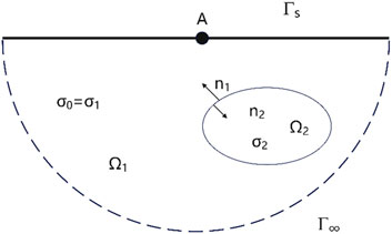
Figure 1. Uneven geoelectric cross section (Xu, 1994). (A: the point source; ${\sigma }_1$: the conductivity of the background medium; ${\sigma }_2$: the conductivity of the anomalous body; ${\mathrm{\Gamma }}_S$: the surface boundary; ${\mathrm{\Gamma }}_{\infty }$: the infinite boundary; ${\mathrm{\Omega }}_1$: the region filled by ${\sigma }_1$; ${\mathrm{\Omega }}_2$: the region filled by ${\sigma }_2$; ${\mathrm{n}}_1$: the outward direction of ${\mathrm{\Omega }}_1$; ${\mathrm{n}}_2$: the outward direction of ${\mathrm{\Omega }}_2$).

Let the region Ω consist of the ground boundary ${\mathrm{\Gamma }}_s$ and the subsurface boundary ${\mathrm{\Gamma }}_{\infty }$. When an anomalous body with conductivity σ₂ appears in the σ₁ medium, the conductivity of the surrounding medium is set as σ₁ = σ₀. σ₀ is the conductivity of the medium where the power supply is located. Ω₁, Ω₂, u₁, u₂ represent the areas where σ₁, σ₂ are located and the anomalous potential.

The relationship between the potentials u₁ and u₂ at two points infinitely close on both sides of the regions Ω₁ and Ω₂ is (Equation 8):

$u_1=u_2(8)$

At the interface, the normal component of the current density perpendicular to the interface is equal (Equation 9).

${\sigma }_1\frac{\mathrm{\partial }{u}_1}{\mathrm{\partial }\mathrm{n}}=-{\sigma }_2\frac{\mathrm{\partial }{u}_2}{\mathrm{\partial }\mathrm{n}}(9)$

Where n represents the normal direction of the interface.

On the ground surface, the normal component of the potential is zero (Equation 10) (Lv, 2008).

$\frac{\mathrm{\partial }u}{\mathrm{\partial }\mathrm{n}}=0\in {\mathrm{\Gamma }}_s(10)$

At the infinite boundary Γ_∞, the mixed boundary conditions are satisfied (Equation 11) (Lv, 2008).

$\frac{\mathrm{\partial }u}{\mathrm{\partial }\mathrm{n}}+\frac{\cos \left(r,n\right)}{r}u=0\in {\mathrm{\Gamma }}_{\infty }(11)$

In the above equation, r represents the distance between A and the spatial boundary, and n denotes the outward normal direction of the spatial boundary.

This leads to the differential equation for u and its boundary conditions (Equation 12) (Wang, 2015):

$\left\{\begin{array}{ll}\frac{\mathrm{\partial }u}{\mathrm{\partial }\mathrm{n}}=0& \in {\mathrm{\Gamma }}_s\\ u_1=u_2& \in \mathrm{\Gamma }\\ {\sigma }_1\frac{\mathrm{\partial }{u}_1}{\mathrm{\partial }{\mathrm{n}}_1}+{\sigma }_2\frac{\mathrm{\partial }{u}_2}{\mathrm{\partial }{\mathrm{n}}_2}=-\left({\sigma }_2\frac{\mathrm{\partial }{u}_0}{\mathrm{\partial }{\mathrm{n}}_1}+{\sigma }_2\frac{\mathrm{\partial }{u}_0}{\mathrm{\partial }{\mathrm{n}}_2}\right)& \in \mathrm{\Gamma }\\ \frac{\mathrm{\partial }u}{\mathrm{\partial }\mathrm{n}}+\frac{\cos \left(r,n\right)}{r}u=0& \in {\mathrm{\Gamma }}_{\infty }\\ \nabla ·\left(\sigma u\right)=-\nabla ·\left({\sigma }^{\prime }{u}_0\right)& \end{array}\right.(12)$

In the equation, σ represents the electrical conductivity of the underground space, while ${\sigma }^{\prime }$ represents its residual conductivity value.

By transforming it into a variational problem, we obtain (Equation 13) (Wang, 2015):

$\left\{\begin{array}{l}F\left(u\right)={\int }_{\mathrm{\Omega }}\left[1/2\sigma {\left(\nabla u\right)}^2+{\sigma }^{\prime }\nabla u_0·\nabla u\right]d\mathrm{\Omega }+{\int }_{\mathrm{\Gamma }\infty }\frac{\sigma u^2\cos \left(r,n\right)}{2r}\\ +\frac{{\sigma }^{\prime }{u}_{0}u\cos \left(r,n\right)}{r}d\mathrm{\Gamma }\\ \sigma F\left(u\right)=0\end{array}\right.(13)$

2.3 Equivalent resistivity method

According to Seigel’s theory (Seigel, 1959), in forward simulation, the primary field potential is solved first. Then, using the equivalent resistivity method, the original model’s anisotropic resistivity ρ is replaced by the equivalent resistivity ρ*, and a second calculation is performed to obtain the total field potential (polarization field potential). The secondary field potential is obtained by subtracting the primary field potential from the total field potential.

Where ρ*_s represent the equivalent apparent resistivity, ρ_s represent the apparent resistivity, η represent the anisotropic polarization rate, η_s represent the apparent polarization rate, and K represent the device coefficient.

The corresponding theoretical expressions are as follows (Equations 14–17):

${\rho }^{*}=\frac{\rho }{1-\eta }(14)$

${\rho }_s=K\frac{\Delta U_1}{I}(15)$

${\rho }_s^{*}=K\frac{\Delta U}{I}(16)$

${\eta }_S=\frac{\Delta U_2}{\Delta U}\times 100\%=\frac{\Delta U-\Delta U_1}{\Delta U}\times 100\%=\frac{{\rho }_s^{*}-{\rho }_s}{{\rho }_s^{*}}\times 100\%(17)$

2.4 Three-dimensional forward modeling theory of SBIP

In Figure 2, the potentials at the vertices of the tetrahedron are represented, and the potential at any point inside the tetrahedron can be obtained as u (Equation 18):

$u=\sum _{i=1}^4{N}_i{u}_i(18)$

$N_i$ is the shape function, which represents the volume ratio of the two tetrahedrons.

Figure 2

Figure 2. Tetrahedral structure.

The element matrices are assembled into the global matrix. By integrating the four terms in the variational formation of the anomalous potential method (Equation 13), the following can be obtained (Equation 19):

$F\left(u\right)=\sum \left(\frac{\sigma }{2}{u}^T{K}_{1e}u+{\sigma }^{\prime }{u}^T{K}_{1e}{u}_0+\frac{\sigma }{2}{u}^T{K}_{2e}u+{\sigma }^{\prime }{u}^T{K}_{2e}{u}_0\right)=\frac{1}{2}{u}^{T}Ku+u^T{K}^{\prime }{u}_0(19)$

Setting the variation of the above equation to zero, the following is obtained (Equation 20):

$Ku=K^{\prime }{u}_0(20)$

Equation 20 is solved using the improved symmetric successive over-relaxation preconditioned conjugate gradient iteration algorithm (SSOR-PCG) (Lin, 1998). For Ax = b, matrix A is set as an n - order symmetric positive definite matrix, and the preconditioning matrix M is represented as (Equation 21):

$M={\left(2-\omega \right)}^{-1}\left(\frac{D}{\omega }+L\right){\left(\frac{D}{\omega }\right)}^{-1}{\left(\frac{D}{\omega }+L\right)}^T(21)$

For the above equation: D is the diagonal matrix of A; L is the lower triangular matrix of A; $\mathrm{\omega }$ is the relaxation factor, which is a constant between 0 and 2.

Assuming the source is a point on the surface, and the subsurface conductivity σ = σ₀, the normal potential u₀ is (Equation 22):

$\nabla ·\left({\sigma }_0\nabla u_0\right)=-2I\delta \left(A\right)(22)$

The normal potential u₀ can be calculated analytically from Equation 23, while the anomalous potential is obtained by solving Equation 20. The sum of both gives the total potential value (Equation 23).

$u_0=\frac{\rho I}{4\pi R}(23)$

Where R represents the distance between the receiver point and the source point. It is important to note that ρ is in tensor form at this point.

3 Algorithm validation

3.1 Isotropic sphere model

This paper validates the accuracy of the surface-borehole induced polarization algorithm by constructing a uniform isotropic low-resistivity spherical model. The constructed spherical model is shown in Figure 3, where the surrounding rock has a resistivity of 100 Ω m (high-resistivity surrounding rock), and the anomaly is a 10 Ω m low-resistivity sphere (radius 1 m). The anomaly is buried at a depth of 10 m, with its center located 2 m from the borehole. The source is set 10 m from the borehole entrance on the surface, and the measurement line is located inside the borehole with 30 measurement points, spaced 1 m apart. The measurements were conducted using a three-electrode array configuration. The error analysis is performed by comparing the three-dimensional forward modeling results in this paper with the analytical solution to verify its accuracy (Lv, 2008).

Figure 3

Figure 3. Schematic diagram of a three-dimensional complex isotropic Surface-borehole spherical model.

The comparison results are shown in Figure 4. The three-dimensional forward modeling results in this paper fit very well with the analytical solution, with the maximum absolute error being only 1.2%, indicating that the azimuthal surface-borehole induced polarization forward modeling algorithm proposed in this paper has good accuracy and effectiveness.

Figure 4

Figure 4. Comparison of numerical and analytical solutions.

4 The response of BSIP

The forward simulation of the SBIP method, considering electrical anisotropy, was implemented using the geoelectric model shown in Figure 5 (other azimuthal surface-borehole models are designed according to different distances from the borehole entrance). The source A0 is set at the coordinates (0, 0, 0), which is also the location of the borehole. The anomaly is set at a depth of 610 m underground, 70 m from the borehole (measurement line), and the specific size of the anomaly is 100 m × 100 m × 50 m. The measurement line is arranged in a vertical downward direction, with the first measurement point located 450 m from the borehole entrance and the last measurement point 750 m from the borehole entrance. The distance between measurement points MN is 2 m. The measurements were conducted using a three-electrode array configuration.

Figure 5

Figure 5. Schematic diagram of Surface-borehole induced polarization model.

The surface source azimuth distribution is shown in Figure 6, where the azimuth A0 is located at the borehole entrance, A1 (200,0,0) is the primary azimuth, A2 (-200,0,0) is the reverse azimuth, and the other two azimuths, A3 (0,200,0) and A4 (0, −200,0), are auxiliary azimuths. The distance L from the azimuth to the borehole entrance is 200 m.

Figure 6

Figure 6. Schematic diagram of the azimuth distribution of Surface-boreholes (A0 (0,0,0), A1 (200,0,0), A2 (-200,0,0), A3 (0,200,0), A4 (0,-200,0)).

This paper uses a free tetrahedral mesh to discretize the model. To improve accuracy, local mesh refinement is applied at the source, measurement line, and anomaly locations. The number of mesh divisions for different azimuth models is shown in Table 1. The mesh discretization is shown in Figure 7 (Azimuths A3 and A4 have the same azimuth characteristics relative to the anomaly, and the observation results are consistent; therefore, only the A3 model is shown).

Table 1

Table 1. Mesh generation results in different directions.

Figure 7

Figure 7. Azimuth Surface-borehole model meshing diagram (a) A0 azimuth model meshing map; (b) A1 azimuth model meshing map; (c) A2 azimuth model meshing map; (d) A3 azimuth model meshing map.

4.1 Principal axis isotropic media

Before conducting the study of electrical anisotropy characteristics, it is necessary to perform a preliminary analysis of the response characteristics under isotropic conditions. Therefore, an isotropic surrounding rock and anomaly are set for the surface-borehole five-azimuth model, with the isotropic conductivity tensors set as follows: $\sigma =\left(\begin{array}{ccc}0.01& 0& 0\\ 0& 0.01& 0\\ 0& 0& 0.01\end{array}\right)S·m^{-1}$, $\sigma =\left(\begin{array}{ccc}1& 0& 0\\ 0& 1& 0\\ 0& 0& 1\end{array}\right)S·m^{-1}$

The polarization tensor of the anomaly’s principal axis with isotropic polarization rate is: $\eta =\left(\begin{array}{ccc}0.5& 0& 0\\ 0& 0.5& 0\\ 0& 0& 0.5\end{array}\right)$. The polarization rate of the surrounding rock is not considered, and the current is 50 A.

Figures 8, 9 show the forward modeling results of the surface-borehole azimuthal induced polarization model under isotropic conditions. Analyzing the surface-borehole azimuthal IP response helps understand the characteristics of the observed anomaly curves. The anomalous field caused by a horizontal plate-like body can be considered as the result of the combined effect of multiple dipole fields (Lv et al., 2012). From the anomaly curves, we can see the response characteristics of sources in different directions to anomalous bodies. When observing A0 azimuth, the influence of anomalous body can be regarded as the function of vertical electric dipole field, and the abnormal curves of apparent resistivity and apparent polarizability are symmetrically distributed. At the center of anomalous body, the direction of anomalous field is opposite to that of normal field, and both apparent resistivity and apparent polarizability will have extreme values. Near the upper and lower boundaries of the anomalous body, the direction of the anomalous field is the same as that of the normal field, and the anomalous curve as a whole shows the opposite characteristics of high resistance and low polarization. When observed in A1 azimuth, the influence of the anomaly can be regarded as the action of an inclined electric dipole field, and the anomaly curve is not symmetrical. Above the center of the anomaly, the anomaly field is opposite to the normal field, resulting in low resistance and high polarization anomaly. Near the center of the anomaly, the apparent resistivity is the smallest and the apparent polarizability is the largest. Near the lower boundary of the anomalous body, the anomalous field is in the same direction as the normal field, and there are high resistance and negative polarization. When observed in A2 azimuth, the response of anomalous body is opposite to that in A1 azimuth. When observing in A3 and A4 directions, the influence of the anomaly can be equal to that of the vertical electric dipole field, so it is basically consistent with the result of A0 response.

Figure 8

Figure 8. Anomalous curve of apparent resistivity in isotropic media.

Figure 9

Figure 9. Anomalous curve of apparent polarizability in isotropic media.

4.2 Anomalous body with isotropic polarizability and anisotropic conductivity in principal axes

First, the polarization axis of the anomaly is set to be isotropic, while its conductivity characteristics are set to be anisotropic. In this case, the conductivity tensor of the anomaly in the surface-borehole azimuthal model is represented by $\sigma =\left(\begin{array}{ccc}0.02& 0& 0\\ 0& 1& 0\\ 0& 0& 1\end{array}\right)S·m^{-1}$, $\sigma =\left(\begin{array}{ccc}1& 0& 0\\ 0& 0.02& 0\\ 0& 0& 1\end{array}\right)S·m^{-1}$, $\sigma =\left(\begin{array}{ccc}1& 0& 0\\ 0& 1& 0\\ 0& 0& 0.02\end{array}\right)S·m^{-1}$. While, its polarization tensor is set as: $\eta =\left(\begin{array}{ccc}0.5& 0& 0\\ 0& 0.5& 0\\ 0& 0& 0.5\end{array}\right)$. It should be noted that the surrounding rock is isotropic, with electrical properties as follows: the conductivity is $0.01S·m^{-1}$ and the polarization is 0. The current is 50 A. A comparative analysis is conducted on the apparent resistivity and apparent polarization response characteristics when the conductivity is anisotropic in different azimuths.

Figure 10 shows the apparent resistivity and apparent polarization curves of the principal axis anisotropy of the anomalous body conductivity when the source is in the A0 direction. From the apparent resistivity curve on the left side of Figure 10, it can be seen that the response characteristics are almost identical to the isotropic response, with little change in the primary field. Only when the anomalous body conductivity is anisotropic in the x-axis direction, the apparent resistivity response shows slight differences compared to the isotropic anomalous body. From the apparent polarization curve on the right side of Figure 10, it can be seen that when the anomalous body apparent polarization is anisotropic in the x-axis direction, the apparent polarization changes significantly compared to the isotropic case. At the center of the anomalous body, the apparent polarization increases, exhibiting high polarization anomalies, while above the anomalous body, the apparent polarization slightly decreases. When the anomalous body conductivity is anisotropic in the z-axis direction, the response change in the apparent polarization is the most significant. At the center of the anomalous body, the apparent polarization undergoes a noticeable jump, reaching up to six times that of the isotropic anomalous body, showing a high polarization anomaly. Moreover, the apparent polarization also exhibits significant deviation below and above the anomalous body. Therefore, when the anomalous body conductivity is anisotropic in the z-axis direction, the response effect on the apparent polarization is the most significant, because the anisotropic high resistance direction is consistent with the current diffusion direction, followed by the x-axis direction, while the y-axis direction has little effect. This is because the anisotropy in the horizontal direction has little influence on the current that diffuses vertically downward. The anisotropy of each principal axis does not significantly affect the apparent resistivity. The reason is that the A0 direction is closest to the anomalous body, and there is no good coupling relationship between the current diffusion direction and the anisotropy direction of the three principal axes, so the anisotropy of the principal axes has no great influence on the apparent resistivity.

Figure 10

Figure 10. A0 azimuth conductivity anisotropy anomaly plot (Left: apparent resistivity, right: apparent polarizability).

Figure 11 shows the apparent resistivity and apparent polarization curves of the anomalous body conductivity anisotropy when the source is in the A1 direction. In the apparent resistivity anomaly curve, the anisotropy response characteristics in different directions show significant differences. When the anomalous body conductivity is anisotropic in the y-axis direction, there is no obvious change in the apparent resistivity curve. When the anomalous body conductivity is anisotropic in the x-axis direction, the apparent resistivity curve shows some changes, with a slight increase in resistivity above the anomalous body and a slight decrease below it. The fundamental reason is that the x-axis anisotropy is basically parallel to the current diffusion direction. When the anomalous body conductivity is anisotropic in the z-axis direction (high resistivity in the z-axis), the apparent resistivity shows significant changes. At the center of the anomalous body, there is a large increase in resistivity, and the peak value shifts upward. Above the anomalous body, the resistivity decreases, and below the anomalous body, the resistivity first slightly increases and then decreases. Similarly, the anisotropy in the z-axis direction is basically parallel to the current diffusion direction. In the apparent polarization anomaly response curve, the anisotropic conductivity of the anomalous body in the x-axis and z-axis directions shows significant differences compared to the isotropic case, with a clear second-field response change. At the center of the anomalous body, the apparent polarization significantly increases, showing high polarization anomalies. Below the anomalous body, the apparent polarization decreases, showing low polarization anomalies, and the decrease is more significant in the z-axis direction than in the x-axis direction. Above the anomalous body, the apparent polarization increases in the x-axis direction, while it decreases in the z-axis direction. This shows that the high resistance of anomalous body in z-axis direction is basically parallel to the diffusion direction of current, so it has the greatest influence and the response effect is the most obvious.

Figure 11

Figure 11. A1 azimuth conductivity anisotropy anomaly plot (Left: apparent resistivity, right: apparent polarizability).

Figure 12 shows the apparent resistivity and apparent polarization curves of the anomalous body conductivity anisotropy when the source is in the A2 direction. In the apparent resistivity anomaly curve, the apparent resistivity response shows noticeable changes when the anomalous body conductivity is anisotropic in the x-axis direction. At the center of the anomalous body, the resistivity slightly increases. Above the anomalous body, the resistivity decreases, and below it, the resistivity increases, with the low resistivity peak shifting slightly upward. When the anomalous body conductivity is anisotropic in the z-axis direction, the change in apparent resistivity compared to the isotropic anomalous body is the most significant. At the center of the anomalous body, the resistivity increases noticeably, and the depth corresponding to the lowest resistivity value is deeper than that at the center of the anomalous body. Above and below the anomalous body, the resistivity decreases compared to the isotropic case. In the apparent polarization anomaly curve, when comparing A1 and A2 orientations, it is consistent that the electrical anisotropy in the y-direction does not cause significant changes in apparent polarization. However, the anisotropy in the x-axis and z-axis directions is more prominent, with apparent polarization increasing at the center of the anomalous body, showing high polarization anomalies. The changes in the z-axis direction are stronger than those in the x-axis direction. Above and below the anomalous body, the anisotropy in the x-axis and z-axis directions affects the apparent polarization differently. In the x-axis direction, the apparent polarization above the center suddenly decreases, and below the center, it slightly increases. In the z-axis direction, the apparent polarization decreases both above and below the center, showing small minimum values. As far as apparent resistivity and apparent polarizability are concerned, the response laws of A2 azimuthal anisotropy and A1 azimuthal anisotropy are basically the same. So the mechanistic analysis will not be elaborated herein.

Figure 12

Figure 12. A2 azimuth conductivity anisotropy anomaly plot (Left: apparent resistivity, right: apparent polarizability).

Figure 13 shows the apparent resistivity and apparent polarization curves of the anomalous body conductivity anisotropy when the source is in the A3 and A4 directions. In the apparent resistivity anomaly curve, the anisotropy in the x-axis and y-axis directions does not show significant features, but when the anomalous body conductivity is anisotropic in the x-axis direction, there are slight differences above and below the anomalous body. The response changes most significantly when the anomalous body conductivity is anisotropic in the z-axis direction. At the center of the anomalous body, the resistivity increases significantly compared to the isotropic case, and above and below the anomalous body, the resistivity decreases compared to the isotropic case. In the apparent polarization anomaly curve, by comparing the apparent polarization anomaly curves of A3, A4, and A0 orientations, it can be found that the anomaly curves are almost unchanged. Therefore, the anomalous body conductivity anisotropy in the A3 and A4 orientations has the same impact characteristics as in the A0 orientation.

Figure 13

Figure 13. A3. A4 azimuth conductivity anisotropy anomaly plot (Left: apparent resistivity, right: apparent polarizability).

4.3 Anomalous body with anisotropic polarizability and isotropic conductivity in principal axes

When the conductivity principal axis of the anomalous body is isotropic and the polarization principal axis is anisotropic, the polarization tensor of the anomalous body in the surface-borehole azimuthal model is represented as $\eta =\left(\begin{array}{ccc}0.2& 0& 0\\ 0& 0.5& 0\\ 0& 0& 0.5\end{array}\right)$, $\eta =\left(\begin{array}{ccc}0.5& 0& 0\\ 0& 0.2& 0\\ 0& 0& 0.5\end{array}\right)$, $\eta =\left(\begin{array}{ccc}0.5& 0& 0\\ 0& 0.5& 0\\ 0& 0& 0.2\end{array}\right)$. Here, its conductivity tensor is set to $\sigma =\left(\begin{array}{ccc}1& 0& 0\\ 0& 1& 0\\ 0& 0& 1\end{array}\right)S·m^{-1}$. The other conditions remain the same as previously mentioned. In actual research, it is clear that the polarization anisotropy characteristics of the subsurface anomalous body are not related to the forward calculation of apparent resistivity. Therefore, only the analysis of the anomalous body’s apparent polarization response is considered here.

Figure 14 shows the apparent polarization curves of the anomalous body under different azimuth sources. Figure 14a shows the apparent polarization curve under A0 azimuth source. From the figure, it can be seen that when the polarization anisotropy is along the x-axis, an apparent polarization extreme value appears at the center of the anomalous body, with the maximum value decreasing to some extent compared to the isotropic anomalous body. Also, the apparent polarization slightly increases above the anomalous body and slightly decreases below it. When the polarization anisotropy is along the y-axis, the apparent polarization response is almost the same as when it is isotropic, with only a slight increase at the position of the maximum value. When the polarization anisotropy is along the z-axis, the effect on the apparent polarization is the greatest, leading to a significant decrease in the maximum apparent polarization at the center of the anomalous body, and an increase in apparent polarization to some extent above and below the anomalous body.

Figure 14

Figure 14. Polarizability anisotropy apparent polarizability anomaly plot (a) A0 azimuth; (b) A1 azimuth; (c) A2 azimuth; (d) A3. A4 azimuth.

Figure 14b shows the apparent polarization curve under A1 azimuth source. From the figure, it can be observed that the polarization anisotropy along the principal axis of the anomalous body in the A1 azimuth results in the most significant changes in the apparent polarization curve. The polarization anisotropy along different principal axes causes the maximum value of the apparent polarization curve to shift upwards. The shift is most pronounced along the z-axis, followed by the y-axis, while the shift along the x-axis is not obvious. Although the shift of the extreme value along the z-axis is relatively large, the magnitude of the extreme value does not change significantly. However, for anisotropy along the x and y-axes, the extreme value increases substantially, with the increase being most notable for the y-axis, resulting in a high polarization anomaly. Above the anomalous body, the anisotropy along the y and z-axes causes a considerable increase in the apparent polarization, while below the anomalous body, anisotropy in all three directions leads to the appearance of an apparent polarization minimum.

Figure 14c shows the apparent polarization curve under A2 azimuth source. From the figure, it can be seen that the anisotropy along the y-axis does not result in significant changes. When there is polarization anisotropy along the x-axis, the maximum value of the apparent polarization decreases, and the position of the maximum value shifts slightly upwards. The apparent polarization increases above the anomalous body and decreases below it. When there is anisotropy along the z-axis, the change in the apparent polarization curve is most significant, with the maximum value decreasing substantially, and the position of the maximum value shifting significantly downwards. Below the anomalous body, the apparent polarization increases, while the change above the anomalous body is not significant.

Figure 14d shows the apparent polarization response curve under A3 and A4 azimuth sources. From the figure, it can be seen that the effect of polarization anisotropy on the apparent polarization curve is minimal for A3 and A4 azimuths. The effect is only noticeable when there is anisotropy along the z-axis, where the extreme value of the apparent polarization decreases significantly, and the apparent polarization slightly increases below the anomalous body. Anisotropy along the x and y-axes only leads to a slight decrease in the extreme value of the apparent polarization.

4.4 Anomalous body with anisotropic polarizability and anisotropic conductivity in principal axes

When the principal axis of the conductivity of the anomalous body is anisotropic and the principal axis of the polarization is also anisotropic, the conductivity tensor of the anomalous body in the surface-borehole azimuth model is represented by $\sigma =\left(\begin{array}{ccc}0.02& 0& 0\\ 0& 1& 0\\ 0& 0& 1\end{array}\right)S·m^{-1}$, $\sigma =\left(\begin{array}{ccc}1& 0& 0\\ 0& 0.02& 0\\ 0& 0& 1\end{array}\right)S·m^{-1}$, $\sigma =\left(\begin{array}{ccc}1& 0& 0\\ 0& 1& 0\\ 0& 0& 0.02\end{array}\right)S·m^{-1}$. And the polarization tensor of the anomalous body in the azimuth borehole model is represented by $\eta =\left(\begin{array}{ccc}0.2& 0& 0\\ 0& 0.5& 0\\ 0& 0& 0.5\end{array}\right)$, $\eta =\left(\begin{array}{ccc}0.5& 0& 0\\ 0& 0.2& 0\\ 0& 0& 0.5\end{array}\right)$, $\eta =\left(\begin{array}{ccc}0.5& 0& 0\\ 0& 0.5& 0\\ 0& 0& 0.2\end{array}\right)$, and the surrounding rock and source emission information remain consistent with the previously mentioned models. Similarly, only the analysis of the response of the apparent polarization is considered here.

Figure 15a shows the response curve of the apparent polarization when the principal axes of the anomaly body’s conductivity and polarization are anisotropic during A0 azimuth source. From the figure, it can be seen that the anisotropy in the x-direction causes an increase in the maximum value of the apparent polarization, while the apparent polarization shows a minimum value at the upper and lower positions of the anomaly body. The anisotropy in the z-direction results in a decrease in the maximum value of the apparent polarization compared to isotropic conditions, while the apparent polarization slightly increases at the upper and lower positions of the anomaly body. Figure 15b shows the response curve of the apparent polarization when the principal axes of the anomaly body’s conductivity and polarization are anisotropic during A1 azimuth source. It can be seen from the figure that in both the x and z directions, the maximum value of the apparent polarization when the conductivity and polarization are anisotropic is greater than in the isotropic case, with the z-direction anisotropy showing a larger increase. However, the anisotropy in the z-direction causes a decrease in the apparent polarization above the anomaly body. Figure 15c shows the response curve of the apparent polarization when the principal axes of the anomaly body’s conductivity and polarization are anisotropic during A2 azimuth source. Similar to the A1, in the x and z directions, the maximum value of the apparent polarization when conductivity and polarization are anisotropic is larger than in the isotropic case, with a greater increase in the z-direction. However, different from the A1, the anisotropy in the x and z directions causes a decrease in the apparent polarization above the anomaly body, resulting in a minimum value, which is shown as a low polarization anomaly. Below the anomaly body, the z-direction anisotropy causes a decrease in the apparent polarization, with no obvious effect from the x-direction anisotropy. Figure 15d shows the response curve of the apparent polarization when the principal axes of the anomaly body’s conductivity and polarization are anisotropic during A3 and A4 azimuth sources. From the figure, it can be seen that for both A3 and A4, when the conductivity and polarization are anisotropic in the x and z directions, the maximum value of the apparent polarization is greater than in the isotropic case, with the z-direction anisotropy showing a larger increase. However, the difference is that the anisotropy in both the x and z directions cause a decrease in the apparent polarization above and below the anomaly body, with the minimum value being smaller in the z-direction anisotropy. It is worth noting that for any orientation of the anomaly body, the response curve of the apparent polarization under anisotropy in the y-direction for conductivity and polarization is almost identical to that of the isotropic anomaly body. It is because the anisotropy in the y-axis direction has little influence on the vertical downward diffusion current, the anisotropy in the x-axis has a greater influence than the anisotropy in the y-axis, and the anisotropy in the z-axis has the same high resistance as the current diffusion direction, so it has the greatest influence.

Figure 15

Figure 15. Conductivity, polarizability, anisotropy apparent polarizability anomaly plot (a) A0 azimuth; (b) A1 azimuth; (c) A2 azimuth; (d) A3. A4 azimuth.

5 Conclusion

This paper is based on the anomalous potential method and the equivalent resistivity theory. By introducing the tensor conductivity of principal axis anisotropic media, a three-dimensional forward modeling of the borehole-surface induced polarization method for principal axis electrical anisotropic media is implemented using the finite element method. The correctness of the algorithm is verified using a uniform isotropic borehole spherical model. Considering the cases where both the conductivity and polarizability of the anomalous body are anisotropic, the response characteristics of apparent resistivity and apparent polarizability under different azimuth sources are analyzed.

1. When the anomalous body exhibits principal-axis electrical anisotropy in conductivity and isotropy in polarizability, the apparent resistivity curve at azimuth A0 is essentially consistent with that of the isotropic case, except that the minimum value of the curve is slightly higher than the isotropic case when the anomalous body is anisotropic along the x-axis. In contrast, the apparent polarizability curve is most significantly affected when the anomalous body is anisotropic along the z-axis, followed by the x-axis anisotropy, both leading to an increase in the peak value of the apparent polarizability. However, anisotropy along the y-axis has almost no influence. At azimuth A1, when the anomalous body exhibits x-axis anisotropy, the minimum value of the apparent resistivity curve is slightly higher than that in the isotropic case. Meanwhile, the apparent polarizability curve first reaches a maximum before decreasing to a minimum. In contrast, y-axis anisotropy has negligible influence on both the apparent resistivity and apparent polarizability curves. When z-axis anisotropy is present, the apparent resistivity curve first reaches a minimum followed by a maximum, while the peak value of the apparent polarizability curve increases significantly (by multiple times). At azimuth A2, both the apparent resistivity and apparent polarizability curves exhibit characteristics generally similar to those observed at A1, but with notable distinctions. Specifically, x-axis anisotropy in the anomalous body causes the apparent polarizability curve to first reach a minimum before rising to a maximum, reversing the trend seen at A1. Meanwhile, z-axis anisotropy leads to an apparent resistivity curve that initially peaks at a maximum before decreasing to a minimum, demonstrating an inverse pattern compared to the A1 response. These variations highlight the azimuth-dependent behavior of anisotropic media in borehole-surface IP surveys. At azimuths A3 and A4, the characteristics of apparent resistivity and apparent polarizability curves are essentially similar to those at azimuth A0, but z-axis anisotropy of the anomalous body causes an increase in the minimum value of the apparent resistivity curve.

2. When the anomalous body exhibits isotropic conductivity along principal axes but anisotropic polarizability, at azimuths A0 and A2, both x-axis and z-axis anisotropies of the anomalous body lead to a reduction in the peak values of the apparent polarizability curves. Notably, the z-axis anisotropy results in a more pronounced decrease in the maximum value of the apparent polarizability curve compared to x-axis anisotropy. When the anomalous body exhibits y-axis anisotropy, the apparent polarizability curve remains consistent with that of the isotropic case. At azimuth A1, both x-axis and y-axis anisotropies of the anomalous body lead to an increase in the maximum values and a decrease in the minimum values of the apparent polarizability curves. Notably, the y-axis anisotropy induces more significant variations in both the maximum and minimum values of the apparent polarizability curve compared to x-axis anisotropy. In contrast, z-axis anisotropy causes an upward shift in the extreme values of the apparent polarizability curve. At azimuths A3 and A4, the x-axis, y-axis, and z-axis anisotropies of the anomalous body all result in a reduction of the maximum values in the apparent polarizability curves. Notably, the z-axis anisotropy produces the most significant reduction in the curve’s peak value. The apparent polarizability curves for x-axis and y-axis anisotropies completely overlap, with their maximum values being lower than those observed in the isotropic case.

3. When the anomalous body exhibits principal-axis electrical anisotropy in both conductivity and polarizability, at azimuth A0, x-axis anisotropy increases the maximum value of the apparent polarizability curve while z-axis anisotropy decreases it. At azimuths A1, A2, A3, and A4, both x-axis and z-axis anisotropies increase the maximum values of the apparent polarizability curves, with z-axis anisotropy producing larger maximum values. Under all source configurations, the apparent polarizability curves for y-axis anisotropy remain identical to those in the isotropic case.

This study clearly defines the forward response characteristics of the surface-borehole azimuthal induced polarization method under electrical anisotropic conditions. The findings can serve as a theoretical foundation to aid research on borehole electromagnetic methods in anisotropic media.

Data availability statement

The raw data supporting the conclusions of this article will be made available by the authors, without undue reservation.

Author contributions

LZ: Writing – original draft, Conceptualization. TC: Data curation, Writing – review and editing. J-KZ: Writing – review and editing. GC: Software, Writing – review and editing. XW: Methodology, Writing – review and editing. YM: Validation, Writing – review and editing. LY: Project administration, Writing – review and editing.

Funding

The author(s) declare that financial support was received for the research and/or publication of this article. This study was funded by the National Natural Science Foundation of China (42274103, 42030805).

Conflict of interest

Author TC was employed by Sinopec Geophysical Corporation Jianghan Branch.

The remaining authors declare that the research was conducted in the absence of any commercial or financial relationships that could be construed as a potential conflict of interest.

The reviewer YL declared a shared affiliation with the author XW to the handling editor at time of review.

Generative AI statement

The author(s) declare that no Generative AI was used in the creation of this manuscript.

Any alternative text (alt text) provided alongside figures in this article has been generated by Frontiers with the support of artificial intelligence and reasonable efforts have been made to ensure accuracy, including review by the authors wherever possible. If you identify any issues, please contact us.

Publisher’s note

All claims expressed in this article are solely those of the authors and do not necessarily represent those of their affiliated organizations, or those of the publisher, the editors and the reviewers. Any product that may be evaluated in this article, or claim that may be made by its manufacturer, is not guaranteed or endorsed by the publisher.

References

An, R., Deng, C., Qi, X. H., Xiang, M., Zhang, F. W., and Li, J. B. (2018). Application of ground-well induced polarization method to determine bottom hole blind orebody. Coal Technol. 37 (12), 106–108. doi:10.13301/j.cnki.ct.2018.12.038

CrossRef Full Text | Google Scholar

Cai, B. L., Huang, Z. H., and Gu, S. M. (1983). Induced polarization method in borehole, in-hole IP method. Beijing: Geology Press.

Google Scholar

Chambers, J. E., Wilkinson, P. B., Weller, A. L., Meldrum, P. I., Ogilvy, R. D., and Caunt, S. (2007). Mineshaft imaging using surface and crosshole 3D electrical resistivity tomography: a case history from the east pennine coalfield, UK. J. Appl. Geophys. 62 (4), 324–337. doi:10.1016/j.jappgeo.2007.03.004

CrossRef Full Text | Google Scholar

Chen, F. (2022). Application of surface-borehole induced polarization survey in xiangyangping uranium deposit. J. East China Univ. Technol. Nat. Sci. 45 (03), 261–268. doi:10.3969/j.issn.1674-3504.2022.03.007

CrossRef Full Text | Google Scholar

Chen, H. H., Ma, H. L., and Yang, Z. C. (2019). Forward calculation of borehole IP in ground-well mode based on finite difference. Energy Technol. Manag. 44 (03), 10–12. doi:10.3969/j.issn.1672-9943.2019.03.004

CrossRef Full Text | Google Scholar

Chlamtac, M., and Abramovici, F. (1981). The electromagnetic fields of a horizontal dipole over a vertically inhomogeneous and an-isotropic earth. Geophysics 46 (6), 904–915. doi:10.1190/1.1441229

CrossRef Full Text | Google Scholar

Guo, B., Pan, H. P., Yang, H. J., and Yao, J. (2015). The application of the surface-to-borehole induced polarization method to deter-mining the spatial location of the orebody. Geophys. Geochem. Explor. 39 (06), 1167–1175. doi:10.11720/wtyht.2015.6.12

CrossRef Full Text | Google Scholar

Hou, J., Mallan, R. K., and Torres-Verdín, C. (2006). Finite-difference simulation of borehole EM measurements in 3D anisotropic media using coupled scalar-vector potentials. Geophysics 71 (5), G225–G233. doi:10.1190/1.2245467

CrossRef Full Text | Google Scholar

Li, J. L. (2016). Application of the down-hole IP method to a general survey in the jinya gold deposit. Geol. Explor. 52 (05), 924–930. doi:10.13712/j.cnki.dzykt.2016.05.013

CrossRef Full Text | Google Scholar

Li, J. H., and He, Z. X. (2012). Characteristics of electric field response of 3D reservoir development model using ground-well vertical electromagnetic walkaway profile method. Oil Geophys. Prospect. 47 (04), 653–664+682+517. doi:10.13810/j.cnki.issn.1000-7210.2012.04.012

CrossRef Full Text | Google Scholar

Li, X., and Pedersen, L. B. (1991). The electromagnetic response of an azimuthally anisotropic half-space. Geophysics 56 (9), 1462–1473. doi:10.1190/1.1443166

CrossRef Full Text | Google Scholar

Lin, S. Z. (1998). Solving finite element equations by preconditioned conjugate gradient method and programming. J. Hohai Univ. (03), 114–117.

Google Scholar

Liu, Y. J. (2020). Three-dimensional forward modeling and analysis of time-domain electromagnetic data for an anisotropic medium. Wuhan: China University of Geosciences.

Google Scholar

Liu, Y. H., Yin, C. C., Cai, J., Huang, W., Ben, F., Zhang, B., et al. (2018). Review on research of electrical anisotropy in electromagnetic prospecting. Chin. J. Geophys. 61 (08), 3468–3487. doi:10.6038/cjg2018L0004

CrossRef Full Text | Google Scholar

Lv, Y. Z. (2008). The research on 3-D fast forward and inversion of surface-borehole and borehole-surface IP methods. Hunan: Central South University.

Google Scholar

Lv, Y. Z., Ruan, B. Y., and Peng, S. P. (2012). A study on anomaly of surface-borehole direction induced polarization survey. Prog. Geophys. (in Chinese) 27 (01), 201–216. doi:10.6038/j.issn.1004-2903.2011.06.023

CrossRef Full Text | Google Scholar

Mann, J. E. (1965). The importance of anisotropic conductivity in magnetotelluric interpretation. Journal of Geophysical Research 70 (12), 2940–2942. doi:10.1029/jz070i012p02940

CrossRef Full Text | Google Scholar

Mao, Y. R., Guo, Q. M., Xie, X. B., Zhou, L., Yan, L. J., Tong, X. L., et al. (2023). Study on the influence of logging cable impedance on transmit current waveform in borehole induced polarization method. Well Logging Technology, 1–7. doi:10.16489/j.issn.1004-1338.2023.04.006

CrossRef Full Text | Google Scholar

Osiensky, J. L., Belknap, W. J., and Donaldson, P. R. (2006). Superposition ofborehole-to-surface voltage residuals for vadose zone plumedelineation. Journal of Contaminant Hydrology 82 (3-4), 241–254. doi:10.1016/j.jconhyd.2005.10.006

PubMed Abstract | CrossRef Full Text | Google Scholar

Pan, H. P. (2013). The role of borehole induced polarization/resistivity method in the exploration of mineral resources. Geophysical and Geochemical Exploration 37 (04), 620–626. doi:10.11720/j.issn.1000-8918.2013.4.10

CrossRef Full Text | Google Scholar

Pan, H. P., Ma, H. L., Cai, B. L., and Niu, Y. X. (2009). Induced polarization method in borehole, in-hole IP method. Beijing, China.

Google Scholar

Pek, J., and Santos, A. M. (2006). Magnetotelluric inversion for anisotropic conductivities in layered media. Physics of the Earth and Planetary Interiors 158 (2-4), 139–158. doi:10.1016/j.pepi.2006.03.023

CrossRef Full Text | Google Scholar

Seigel, H. O. (1959). Mathematical formulation and type curves for induced polarization. Geophysics 24 (3), 547–565. doi:10.1190/1.1438625

CrossRef Full Text | Google Scholar

Shen, M. C., Ran, J. L., Zhang, J., and Liu, J. Y. (2017). The application of ground well induced polarization logging in a polymetallic deposit in northern Shaanxi. World Nonferrous Metals (01), 92+94.

Google Scholar

Spitzer, K., and Chouteau, M. (2003). A dc resistivity and IP borehole survey at the casa berardi gold mine in northwestern Quebec. Geophysics 68 (2), 453–463. doi:10.1190/1.1567221

CrossRef Full Text | Google Scholar

Su, B. Y., Fujimitsu, Y., Xu, J. L., and Song, J. Y. (2012). A model study of residual oil distribution jointly using crosswell and bore-hole-surface electric potential methods. Applied Geophysics-Springer 9 (1), 19–26. doi:10.1007/s11770-012-0309-5

CrossRef Full Text | Google Scholar

Sun, H., Liu, Y., Wang, Z., Ji, X.J., Zhao, W., and Chen, C. (2024). Influence of two-dimensional electrical anisotropy on dimensionality analysis of magnetotelluric data. Chinese J. Geophys. 67 (12), 4794–4805. doi:10.6038/cjg2023R0020 (in Chinese)

CrossRef Full Text | Google Scholar

Wang, T. (2002). The electromagnetic smoke ring in a transversely isotropic medium. Geophysics 67 (6), 1779–1789. doi:10.1190/1.1527078

CrossRef Full Text | Google Scholar

Wang, Z. (2015). Research on forward and inversion of induced polarization in borehole and application. Wuhan: China University of Geosciences.

Google Scholar

Wang, P. X. (2018). Study on the 3-D forward and inversion of induced-polarization in borehole. Beijing: China University of Geosciences. doi:10.3969/j.issn.1000-1441.2018.06.015

CrossRef Full Text | Google Scholar

Wang, Z., Wu, A. P., and Li, G. (2018). Forward modeling of borehole-ground induced polarization method under undulating topography. Geophysical Prospecting for Petroleum 57 (06), 927–935+951.

Google Scholar

Wilkinson, P. B., Chambers, J. E., Mike, L., Wealthall, G. P., and Ogilvy, R. D. (2008). Extreme sensitivity of crosshole electrical resistivity tomography measurements to geometric errors. Blackwell Publishing Ltd. 173 (1), 49–62. doi:10.1111/j.1365-246X.2008.03725.x

CrossRef Full Text | Google Scholar

Xu, S. Z. (1994). Finite element method in geophysics. Beijing, China: Science Press.

Google Scholar

Xue, B. L., Liu, G. M., Tian, Z. B., Zhao, Q., Ren, L., and Xu, X. X. (2020). Indication significance of in-situ IP in exploration of concealed copper deposits. Geophysical and Geochemical Exploration 44 (03), 507–513. doi:10.11720/wtyht.2020.1445

CrossRef Full Text | Google Scholar

Yan, L. J., Zhou, L., Xie, X. B., and Wang, Z. G. (2014). The transient electromagnetic responsein of electrical anisotropic reservoir model. Chin. J. Eng. Geophys. 11 (03), 346–350. doi:10.3969/j.issn.1672-7940.2014.03.013

CrossRef Full Text | Google Scholar

Yin, C. C. (2010). Geoelectrical inversion for a one-dimensional anisotropic model and inherent non-uniqueness. Geophysical Journal International 140 (1), 11–23. doi:10.1046/j.1365-246x.2000.00974.x

CrossRef Full Text | Google Scholar

Yu, G. (2018). Three-dimensional magnetotelluric forward modeling for arbitrary electrical anisotropic media and practical applications. Institute of Geology, China Earthquake Administration.

Google Scholar

Zhang, G. Y., Lv, Y. Z., Liu, Z., and Zhao, H. P. (2013). Surface-borehole cross-secrion IP method numerical modeling and data Ex-planation. Chin. J. Eng. Geophys. 10 (1), 46–50. doi:10.3969/j.issn.1672-7940.2013.01.010

CrossRef Full Text | Google Scholar

Zhou, N. N., Lei, K. X., Xue, G. Q., and Chen, W. (2020). Induced polarization effect on grounded-wire transient electromagnetic data from transverse electric and magnetic fields. Geophysics 85 (4), E111–E120. doi:10.1190/geo2019-0322.1

CrossRef Full Text | Google Scholar

Zhu, J., Yin, C. C., Ren, X. Y., Liu, Y. H., Hui, Z. J., and Gu, Y. (2021). DC resistivity forward modelling for arbitrarily anisotropic media using the unstructured spectral element method. Chin. J. Geophys. 64 (12), 4644–4657. doi:10.6038/cjg2021P0199

CrossRef Full Text | Google Scholar