Enhancing landslide dam stability prediction: a data-driven framework integrating missing data imputation and optimal threshold discrimination

Introduction: Accurate prediction of landslide dam stability is critical for mitigating downstream hazards, but reliable models are hindered by incomplete inventories due to missing data. This study addresses this gap by integrating advanced imputation techniques with machine learning (ML) to enhance prediction accuracy and applicability.

Methods: We compiled a global inventory of 518 landslide dam cases (25% missing data rate) and evaluated five imputation methods: generative adversarial imputation nets (GAIN), missForest, multiple imputations by chained equations (MICE), K-nearest neighbors (KNN), and mean most-frequency (MMF). Imputed datasets were used to train four ML models (SVM, RF, XGBoost, LR), with GAIN-SVM further optimized via Youden-index-based threshold discrimination.

Results: GAIN achieved the lowest RMSE (0.205) for continuous variables and 66.0% accuracy for categorical data. The GAIN-SVM combination yielded the highest predictive performance (AUC = 0.823), surpassing traditional methods by 15.2%. Threshold optimization improved classification accuracy by 3.1−9.3% for ambiguous cases (probabilities ∼0.5).

Discussion: The framework enables robust stability assessments even with incomplete field data, supporting emergency decision-making in landslide-prone regions. Its integration into early warning systems could enhance risk mitigation in data-scarce areas.

1 Introduction

Landslide dams can cause a significant cascade of geohazards, usually as a result of large-scale slope movements in high and deep valleys (Stefanelli et al., 2015; Zhao et al., 2018). The resulting hazards include damming leading to backwater lasting for several kilometers upstream and dam failure leading to catastrophic flooding downstream (Liao et al., 2018). Statistical results indicate approximately 50% of landslide dams fail within 1 week of formation (Wang and Liu, 2013; Frigerio Porta et al., 2020), and 85% fail within 1 year of formation (Wang and Liu, 2013; Frigerio Porta et al., 2020). Therefore, rapid and accurate evaluation of the stability of landslide dams is important for early identification and hazard management.

Over the past 30 years, much research has been developed on the formation of landslide dams, and a series of methods have been proposed to evaluate the stability of landslide dams (Chen et al., 2014; Fan et al., 2014; Sica et al., 2019). These various complex methods have been used for modeling the stability of landslide dams for the purpose of explaining the factors involved as accurately as possible. These approaches can be roughly included into two types: physically-based approaches, and data-driven techniques (Zheng et al., 2021). The physically-based models concentrate on dam stability from the physical principles of rock-soil stability mechanisms and the quantitative description of the dynamic processes of dam-river interaction (Wang et al., 2013; Li et al., 2020; Nian et al., 2021). Therefore, the physically-based models have a clear, physically interpretable background. However, the high computational requirements and uncertain physical parameters, which are difficult to define properly, are the two main drawbacks of physically-based models (Strom, 2013). Hence, there are limitations in the application of these approaches for the rapid prediction of landslide dam stability. On the contrary, with the development of artificial intelligence, data-driven models have been developed to establish the relationship between the historical inventory of landslide dams and potential driving factors. The research objectives of this kind of study can be generalized into the following three parts: (1) the establishment of a landslide dam inventory database including related factors, (2) the generation of a landslide dam stability assessment framework based on data-driven methods and the hazard-related variables, and (3) the establishment of a discriminant formula for the aim of rapidly evaluating the stability of landslide dams (Liao et al., 2022). However, these data-driven methods critically depend on complete datasets, while real-world landslide dam inventories typically contain a certain number of missing values due to inaccessible terrain and rapid dam failure - a gap that the data-driven methods address through advanced imputation techniques. Early data-driven methods focused on the use of statistical techniques, considering geomorphic parameters with high computational efficiency and a relatively simple structure. Models, such as the I_b (blocked index), I_i (impoundment index), DBI (dimensionless blockage index), etc., were developed using the geometric parameters of the dam and the reservoir capacity (Korup, 2004; Dong et al., 2011; Tacconi Stefanelli et al., 2016). With the development of computer science, such studies now prefer to use the latest machine learning (ML) methods with more complex structures to assess the stability problem of landslide dams, such as logistic regression (LR) (Shan et al., 2020), extreme gradient boosting (XGBoost) (Shi et al., 2022), multilayer perceptrons (MLP) (Song et al., 2022) and Bayesian network (BN) (Tang et al., 2023). These models provide good accuracy in landslide dam stability assessment through novel artificial intelligence techniques, and have been proven to be quite successful in improving the accuracy of predictions. Different from statistical models, ML-based models are inherently non-linear, allowing the use of types of stability correlates factors to be used as input variables. Thus, novel relationships between the correlate factors and the stability state of the landslide dam can be discovered through these approaches.

Data-driven approaches are necessarily data-centric, and the performance of ML algorithms depends on the quality and quantity of available data relevant to the task. However, most of these previous assessments of landslide dam stability have been simulated using complete data sets without missing values (Dong et al., 2011; Chen and Chang, 2015; Stefanelli et al., 2018; Jin et al., 2022). This is because the use of statistical and ML algorithms to perform this task commonly requires complete data. Since 1991, when Costa and Schuster (1991) created a database of 463 landslide dam cases worldwide, a growing number of scientists have created a variety of databases containing more landslide dam cases (Korup, 2004; Tang et al., 2018; Fan et al., 2020; Shen et al., 2020). These databases have provided the basis for the use of a data-driven approach. However, the fact that landslide dams commonly occur in areas such as high mountain valleys makes investigation difficult (Ehteshami-Moinabadi and Nasiri, 2017; Frigerio Porta et al., 2020). These data gaps create critical operational bottlenecks: emergency responders often face 48–72 h delays in risk assessment when waiting for complete field surveys (Wang et al., 2022), while rushed judgments based on partial data increase false alarms by up to 40% (Zheng et al., 2021). In addition, most landslide dams are destroyed within a week of their formation, making it difficult to obtain relevant parameters difficult immediately. The prevalence of incompleteness in the collection of datasets for landslide dam stability assessment is a major challenge for specific applications, as the availability of large consistent datasets is limited. Therefore, our concern in this study stems from the problem of assessing landslide dam stability with missing values. A simple way to achieve completeness is a full case analysis using only observed (non-missing) data values. Current predictions of landslide dam stability are obtained by filtering the data to obtain a complete dataset (Fan et al., 2014; Zheng et al., 2021). This approach is appropriate when a small sample of data contains missing values, e.g., less than 10% or 15% of the total data set is missing and would otherwise produce biased results. Another approach to missing data is the process to estimate values to replace missing values using reasonable approximations learned from the observed data using statistical or machine learning techniques (Emmanuel et al., 2021; Lyngdoh et al., 2022). Simple interpolation methods replace missing values of a variable with a statistical estimate, such as the mean or median of all non-missing values of the variable. These methods replace all missing values in a variable with the same estimated value, thus underestimating the variance of the estimate and resulting in poor performance. In addition, some machine learning (ML) or deep learning (DL) techniques, such as k-nearest neighbors (KNN) (Zhang et al., 2017), artificial neural networks (ANN) (Lin et al., 2022), and decision trees (DT) (Stekhoven and Buhlmann, 2012), techniques are widely used for this purpose and have shown excellent performance. Therefore, in this study, five advanced missing data filling techniques containing one statistically-based, three ML-based, and one DL-based algorithm were introduced to perform missing data padding, namely, mean most-frequency (MMF), KNN, Multiple imputation by chained equations (MICE), missForest, and generative adversarial imputation nets (GAIN). This is because these typical models are widely used in many studies and can well embody the basic features of their corresponding model types (Lobato et al., 2015; Yoon et al., 2018; Arriagada et al., 2021; Mohammadi et al., 2021; Lyngdoh et al., 2022).

The model’s output is a continuous stability probability, which is classified into binary stability states (ST/UT) using the optimal threshold. Here, 0 indicates unstable (UT) and 1 indicates stable (ST) states, aligning with engineering conventions for landslide dam assessment. In the actual process of ML modeling, previous studies often default to using a fixed value of 0.5 as the criterion for judging stability (Dong et al., 2011; Tang et al., 2018; Jin et al., 2022). Although this method has achieved high accuracy in stability prediction in previous studies, there is a lack of research on whether 0.5 can be used as an optimal cut-off value and adapted to all prediction tasks. Therefore, this study proposes an optimal threshold determination method based on the receiver operating characteristic (ROC) curve analysis and Youden index (Monica et al., 2014; Nahm, 2022), subsequently, compares it with the traditional fixed threshold (0.5) to verify its effectiveness.

The purpose of the present study is to develop a framework for predicting the stability of landslide dams. Based on literature research, a total of 518 landslide dam cases from around the world were collected, with a missing rate of approximately 25%. Specifically, our objectives include: (i) the achievement of missing values imputation based on five imputation techniques, (ii) the achievement of landslide dam stability prediction based on four machine learning algorithms, and (iii) the analysis and validation of the performance of different imputation and ML methods by quantitative indices.

2 Materials

2.1 Landslide dam inventory

The inventory of landslide dams plays a critical role in providing detailed dam mass attributes, historical hydrology information, and current dam status. These data provide essential support for data-driven methods for modeling landslide dam stability and assessing the accuracy of prediction results. In the current study, the landslide dam inventory was mainly collected from previous literature, which involves qualitative and quantitative descriptive information of landslide dams (Costa and Schuster, 1991; Tabata et al., 2002; Erimini and Casagli, 2003; Stefanelli et al., 2015; Peng et al., 2016). The inventory was then compared with various landslide dam inventories proposed by other literature, so it can assist in calibrating the inventory information. Ultimately, the inventory compiled for this study includes 1744 landslide dam cases from around the world (Table 1).

Table 1

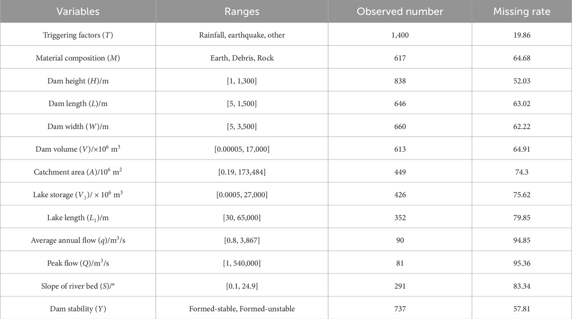
Table 1. Basic information on the landslide dam inventory.

2.2 Landslide dam stability conditioning factors

Landslide dam failure is a complex process, and to date, there is no clear consensus on the exact selection of variables to assess the stability of landslide dams. The conditioning factors of landslide dams can be may be grouped into three categories: dam properties, dam geometric parameters and hydrological factors. According to the characteristics of landslide dams and the available data in the inventory, a total of 12 typical conditioning factors widely applied for landslide dam stability assessment were presented and analyzed (Zheng et al., 2021; Shi et al., 2022). Specifically, these factors can be summarized as dam properties (landslide triggering factors (T), material composition (M)), dam geometric parameters (dam height (H), dam length (L), dam width (W), dam volume (V)), hydrological factors (catchment area (A), lake storage (V₁), lake length (L₁), average annual flow (q), peak flow (Q), slope of river bed (S)).

Landslide dam properties factors reflect the inherent internal characteristics of the dam body. Landslide triggering factors refer to the external forces that contribute to landslide occurrence. In the landslide dam inventory, the triggering factors can be grouped into three categories: heavy rainfall, earthquake and other (human activity, volcano, etc.). Earthquake-triggered landslide dams are generally considered to be more stable than those triggered by rainfall (Chen et al., 2014). This may be due to the fact that rainfall increases the water content of the dam body and thus reduces the shear strength of the soil-rock mass (Wang et al., 2022). Additionally, heavy rainfall increases the flow of the river, causing the water level to rise rapidly and increasing the likelihood of seepage or overtopping damage. The dam material composition factor provides qualitative information on the grain size of the rock-soil masses that make up a landslide dam. In this study, the material composition factor was described as: earth, debris and rock. Dams composed of large blocks of rock have superior stability due to their good supporting function (Mei et al., 2021). Whereas, dams made of loose deposits have lower shear strength and erosion resistance and are more susceptible to damage.

Dam height, dam width and dam length are the basic geometric parameters of a landslide dam, which are the vertical distance between the river bed and the lowest point of the dam top, the length of the dam along the river and the length perpendicular to the river, respectively. Dam volume refers to the volume of the landslide blocking the river section, calculated by the basic geometric parameters.

The catchment area refers to the area of the upstream river where the dam is located, which may reflect the scale of the water flow of the river. The length and volume of the lake are used to describe the magnitude of the upstream barrier lake, and their values will increase with the inflow of water from the upstream after damming (Argentin et al., 2021). The annual average flow and peak flow of rivers reflect the magnitude of the energy of the river impacting the dam, which is generally negatively correlated with dam stability.

2.3 Data preparation

Landslide dams are often formed in mountainous areas where are heavily eroded by rivers. Owing to the complex terrain, many landslide dams were difficult to be discovered, or the recorded landslide inventory was normally not comprehensive. Since there are a lot of missing data in the original landslide dam inventory, we perform some pre-processing at first.

In order to make the best possible use of the information in the database, the landslide dam cases in this study were divided into two categories: available samples and samples in need supplements. The former contains the samples where the sum of the number of dam variables is greater than or equal to three. The latter represents the samples there the sum of the number of dam variables is low than three. The need supplement samples provide too little information to perform the stability assessment of landslide dams.

Hence, for the latter landslide dam samples, they were only recorded until the other information was completed and then will be used to perform the landslide dam stability modeling. A total of 526 cases of landslide dams were collected as the available samples for the following analysis. Among these 526 samples, the missing rate of q, Q and S factors exceed 50%. Research has shown that the high missing rate of a certain variable greatly increases the uncertainty of missing value filling. Thus, for the following analysis, these three factors were first excluded from the available samples. Furthermore, in the propose of using as many influencing factors and complete samples as possible, the available dataset was determined with six factors (M, V, H, L, W and A). For the available dataset, there are 220 complete samples with only observed (no-missing) values, while the remaining 306 samples contain at least one missing value for each case. The total missing rate of the available dataset is approximately 25%. The distribution of missing data across the 526 available samples is shown in Figure 1.

Figure 1

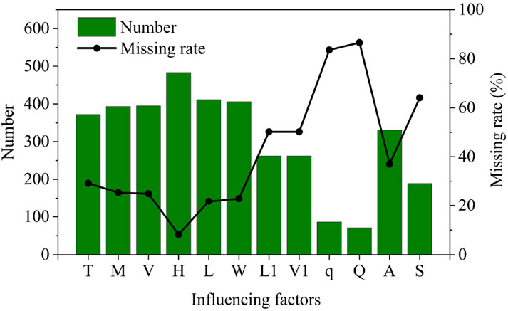
Figure 1. Distribution of missing data in the 526 available samples.

The six selected factors (material composition M, dam volume V, height H, length L, width W, and catchment area A) were prioritized for three reasons: (1) Physical relevance: These parameters collectively represent dam geometry (H, L, W, V), material properties (M), and hydrological forcing (A), which are established controls on stability in prior studies (Ermini and Casagli, 2003; Zheng et al., 2021); (2) Data availability: These factors had observed rates ≤64.9% missing (Table 1), unlike variables like peak flow (Q, 95.4% missing); and (3) Multicollinearity avoidance: VIF analysis confirmed no severe correlations (Section 4.2.1), ensuring model robustness. This balance between physical interpretability and data feasibility supports reliable imputation and prediction.

3 Methodology

To address the challenge of missing data in landslide dam stability prediction, this study develops a comprehensive framework integrating data imputation, machine learning, and threshold optimization. The methodology proceeds in four key stages: (1) preprocessing of the landslide dam inventory to handle missing values and normalize data; (2) evaluation of five imputation techniques (MMF, KNN, MICE, missForest, GAIN) to restore dataset completeness; (3) stability prediction using four machine learning models (SVM, RF, XGBoost, LR); and (4) determination of optimal classification thresholds via the Youden index. The following subsections detail each component, with validation metrics (e.g., RMSE, AUC) used to assess performance at critical stages.

3.1 Miss data imputation methods

3.1.1 Imputation using mean most-frequency (MMF)

In this method, the mean of the observed values is computed for each continuous variable for the missing values for respective variables are imputed by this mean value. For a categorical variable, the missing values are imputed by the most frequent attribute of the observed values. The MMF is a simple imputation method based on the data statistical properties of the data and is easy to implement. However, this method lacks consideration for interdependence of factors and fails to incorporate the inherent uncertainty associated with imputation procedures. This may compromise the validity of any subsequent statistical inference or modeling results that rely on the imputed data.

3.1.2 K-nearest neighbors (KNN)

Clustering is an unsupervised learning technique that relies on the similarity between different samples in the dataset (Zhang et al., 2017). The KNN imputes missing data based on the assumption that similar data points have similar patterns and thus replaces the missing values with the weighted average of the k-nearest neighbors. The weights are computed based on the inverse distance between the incomplete sample and each of its k-nearest neighbors. A higher weight is assigned to a closer neighbor. One major challenge for the configuration of a KNN imputation procedure is determining the optimal number of contributing neighbors, as a low value may lead to oversimplified imputed values, while a high value may smooth over important variations in the data. The KNN method can impute both continuous variables (the mean or weighted mean among of the K-nearest neighbors) and categorical variables (the mode among the K-nearest neighbors) (Sun et al., 2023).

3.1.3 Multiple imputation by chained equations (MICE)

MICE is an imputation approach commonly used in handling missing data in multivariate datasets (Buuren and Groothuis-Oudshoorn, 2011). It offers a comprehensive approach that combines regression models and Monte Carlo simulation to estimate the missing values in a dataset based on the observed values of other variables. This process involves imputing each missing variable sequentially, since, a series of regression models are subsequently created to predict the missing values at each iteration. In the first iteration, the missing value is initially imputed by taking the mean and most frequent of the observed values in the dataset. In the subsequent iterations, the missing values were replaced with the predicted value from the last iteration. Then generate predicted values for the incomplete variable based on its associated imputation model. The iterative process of missing features imputation will be repeated until convergence is achieved. Besides, linear regression, logistic regression and multinomial logistic regression can be interpolated separately in MICE for different variable types such as continuous or categorical variables (Buuren and Groothuis-Oudshoorn, 2011). In summary, MICE is a flexible and widely applicable imputation method. It is attractive in dealing with complex data structures and non-linear relationships between variables.

3.1.4 The missForest algorithm

The missForest algorithm is a multiple imputation approach in mixed-type data using the random forest (RF) algorithm (Stekhoven and Buhlmann, 2012; Feng et al., 2021). Defining a dataset X∈R^n×p, contains n landslide dam cases and p variables, each variable denoted by Xs. For a given variable Xs, it can be separated into two parts: observed values denoted by $Y_{obs}^s$ and missing values denoted by $Y_{mis}^s$. $Y_{obs}^s$ and $Y_{mis}^s$ correspond to m landslide dam cases and the remined n−m cases, respectively. The remined (p−1) variables are also split into two parts: $X_{obs}^s$ and $X_{miss}^s$ which are extracted for the m and n−m cases, respectively. It should be noted that $X_{obs}^s$ and $X_{miss}^s$ can contain both observations and missing values. The goal of missForest is to fill the missing values in $Y_{mis}^s$. The missing value imputation procedure is sorted by first identifying those with less missing data. Then, for each variable, train an RF to fit $Y_{obs}^s$ from $X_{obs}^s$ and then predict the missing values $Y_{mis}^s$ by using the trained RF from $X_{miss}^s$. For the missing values in $X_{obs}^s$ and $X_{miss}^s$, the missForest uses mean imputation or other simple imputation methods as an initial guess at the begin of iteration. Using the built-in out-of-bag error estimates of the RF, one can estimate the imputation error with continuous and category variables that without require a test set. The iterative procedure is repeated until the difference of the newly imputed data and the previous one increases. The $X_{imp}^t$ and $X_{imp}^{t+1}$ are imputed data of t-th and t + 1-th iteration. The difference (Δ) is calculated as follows (Stekhoven and Buhlmann, 2012):

For the continuous variables (Equation 1):

${\Delta }_t=\frac{{\sum }_{i\in X}{\left(X_{imp}^{t+1}-X_{imp}^t\right)}^2}{{\sum }_{i\in X}{\left(X_{imp}^{t+1}\right)}^2}(1)$

And for the category variables (Equation 2):

${\Delta }_t=\frac{{\sum }_{i\in X}{\sum }_{i=1}^n{I}_{X_{imp}^{t+1}\ne X_{imp}^t}}{N}(2)$

where N is the number of missing values in category variables.

3.1.5 Generative adversarial imputation nets (GAIN)

Generative Adversarial Imputation Nets (GAIN) is a powerful framework for imputing missing values using deep learning techniques. In particular, the core components of the GAIN algorithm can be summarized into two parts: a generator network G and a discriminator network D (Yoon et al., 2018). The former network learns the distribution over the observed data and generates imputation samples to fill the missing values. The latter network, D, estimates how well these generated samples match the real data and attempts to recognize which components are actually observed and which are imputed. In G, the input contains three data matrices of the same size, including a data matrix in which missing values were filled with zeros (X^M), a randomly perturbed matrix (R), and a mask matrix (M) recording the locations of the missing data. To reduce redundancy, a hint matrix (H) correlating with the missing pattern is introduced into D with the aim of ensuring discriminator forces the generator, G, to learn the desired distribution (Awan et al., 2021). Then, the adversarial training of the generator and the discriminator is performed, so that the G learns how to generate the more realistic fake samples that can fool the D. This training process repeats iteratively until convergence, at which D finally cannot distinguish the authenticity of the samples generated by the G. For the training process of GAIN, the objective of D is to maximize the probability of correctly predicting M, and for G is to minimize the probability of D predicting M. Thus, the loss function for GAIN is:

$\underset{G}{\min }\underset{D}{\max }V\left(D,G\right)=E_{X,M,H}\left[M^T\log D\left(M\right)+{\left(1-M\right)}^T\log \left(1-M\right)\right](3)$

where log is the element-wise logarithm function, $\widehat{X}$ and $\widehat{M}$ are the outputs of generator and discriminator.

The GAIN architecture was implemented using TensorFlow 2.8 (Python 3.9) on an NVIDIA RTX 3090 GPU. The dataflow architecture of GAIN is illustrated in Figure 2. The GAIN implementation featured: (1) A generator (G) and discriminator (D) with identical 3-layer architectures (256 nodes per layer, LeakyReLU activation, dropout = 0.3); (2) Input processing where missing values were zero-filled (X^M) and combined with a random mask matrix (M) and noise matrix (R); (3) A hint mechanism (H) providing 10% of mask information to D to prevent mode collapse; (4) Training for 50,000 epochs (batch size = 128) using Adam optimizer (l_r = 0.001, β₁ = 0.9, β₂ = 0.999) with gradient penalty (λ = 10); and (5) Early stopping if validation loss plateaued for 1,000 epochs. The loss function (Equation 3) balanced adversarial training (binary cross-entropy) with reconstruction loss (MSE for continuous variables, cross-entropy for categorical). Imputation quality was validated via RMSE on 20% held-out observed values. Training required ∼4.5 h for 50,000 epochs (batch size = 128) on our 518-case dataset, while imputation of missing values took approximately 12 min per experimental run. Hyperparameters included: learning rate = 0.001 (Adam optimizer), generator/discriminator layers = 3 (256 nodes each), and dropout = 0.3. Code and pretrained models are available upon request to ensure reproducibility.

Figure 2

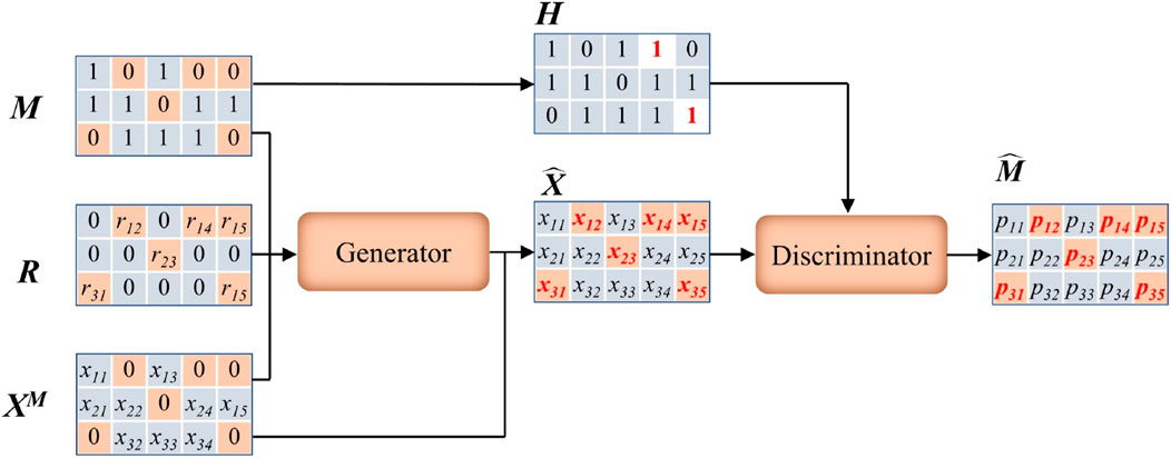
Figure 2. The dataflow of GAIN.

3.2 Support vector machine (SVM)

The SVM model is a multivariable nonlinear predictor with advantages of good generalization performance and the ability to handle high-dimensional data (Cortes and Vapnik, 1995). The principle of structured risk minimization and the theory of statistical learning are the theoretical basis of SVM. The SVM works by mapping the original input data into a higher dimensional space using kernel functions, where it can easier to find a separating hyperplane. The support vectors, which are the points closest to the hyperplane, help to separate the given dataset into classes while minimizing the classification error. This approach allows the SVM to generate an optimal separation boundary with maximum distance from the support vectors, making it robust to noise and outliers.

In the SVM model, three hyperparameters that impacted the prediction performance should be properly determined: the penalty degree, the non-sensitive loss function and the kernel function. To identify the optimal parameter combination, cross-validation and grid search (Qi et al., 2018) methods are adopted in this study. The dataset is splitting into n folds, with one fold reserved for validation and the remaining n−1 folds used for training. A parameter grid containing different hyperparameter values is defined and a grid search algorithm is applied to evaluate all combinations of these hyperparameters based on cross-validation accuracy. The optimal hyperparameters that provide the highest validation accuracy are then selected. Compared to the traditional approach, this method is helpful for overfitting problems and obtaining a more reliable estimate of the model’s performance.

3.3 Landslide dam stability discriminate using youden index

The ROC curve is a commonly used tool for evaluating the performance of binary classification models. It plots the true positive rate (TPR) against the false positive rate (FPR) at different classification thresholds, and provides a visualization of the trade-off between sensitivity (Se) and specificity (Sp) (Fawcett, 2006). Specifically, TPR or Se is the proportion of true positives that are correctly classified as such, while FPR or (1−Sp) is the proportion of false positives that are incorrectly classified as true positives. To draw a ROC curve based on predicted values and actual labels, we first use different thresholds; the confusion matrices can be constructed to calculate multiple TPR and FPR values that can be plotted as points on a ROC curve. The area under the ROC curve (AUC) gives an overall measure of classifier performance ranging from 0 to 1, with higher values indicating greater overall accuracy. The Youden index (J) describes the quantitative relationship between Se and Sp as a function of the classification threshold c (Yin and Tian, 2014). Higher J value indicates higher TPR as well as lower FPR. In other words, the selected cut-off point balances the trade-off between correctly identifying positive cases (high sensitivity) and minimizing false positives (low specificity), under the assuming that equal weighting is given to both types of errors. The optimal cut-off value (c) maximizes the following function (Equation 4) (Monica et al., 2014):

$J\left(c\right)=Se\left(c\right)+Sp\left(c\right)-1(4)$

3.4 Implementation procedure for landslide dam stability estimation

The proposed framework integrates four key phases: (1) Data preprocessing (log transformation, outlier removal via box plots, and min-max normalization); (2) Missing data imputation using five methods (GAIN, missForest, MICE, KNN, MMF) evaluated by RMSE/accuracy metrics; (3) Machine learning modeling with SVM (optimized via grid search over C = [0.1,1,10,100] and γ = [0.001,0.01,0.1,1]), RF, XGBoost, and LR, trained on 70% of data; and (4) Validation using AUC/accuracy metrics and Youden-index-based threshold optimization. All implementations used Python (TensorFlow 2.8 for GAIN; Scikit-learn for other models) with 5-fold cross-validation.

An implementation procedure of the methodology used for developing the landslide dam stability prediction in this study is shown in Figure 3. The main steps in present study are concluded into four parts: data processing, missing data imputation, landslide dam stability modeling and evaluation, and application of the proposed assessment framework to the reality cases. (1) Firstly, in the data processing part, logarithmic transformation was used to reduce the impacts of conditional factors differing by multiple orders of magnitude and the outlier detection using box plot before min-max normalization of the available samples (Jung et al., 2020), and the original data (OM) was generated for the following analysis. The OM, with a missing rate of approximately 25%, contains six the landslide dam conditioning factors and a label for landslide dam stability states. A sub-dataset (C₁) containing all 220 complete samples was then extracted from the OM. (2) In the missing data imputation part, the 25% missing rate was conducted to the C₁ for the aims of simulation the samples collected in reality and the generated new missing dataset, namely, MC. Then five imputation methods (MMF, KNN, MICE, missForest, GAIN) were used to fill the missing component in MC₁, and five different imputation datasets (C_MMF, C_KNN, C_MICE, C_missForest and C_GAIN,) were obtained. (3) In the landslide dam stability modeling part, a total of six different landslide dam datasets (C₁, C_MMF, C_KNN, C_MICE, C_missForest and C_GAIN) were obtained for landslide dam stability prediction modeling. In each dataset, 70% of the samples were randomly selected as the training dataset, and the remaining 30% were used for model validation based on ROC and accuracy analysis. (4) Finally, the landslide dam stability prediction framework will be built based on appropriate imputation method, which was selected to fill the missing values in OM dataset (518 cases), and the SVM will perform the modeling tasks. Furthermore, the Youden method will be used to identify the optimal cut-off point to distinguish formed-unstable and formed-stable landslide dams.

Figure 3

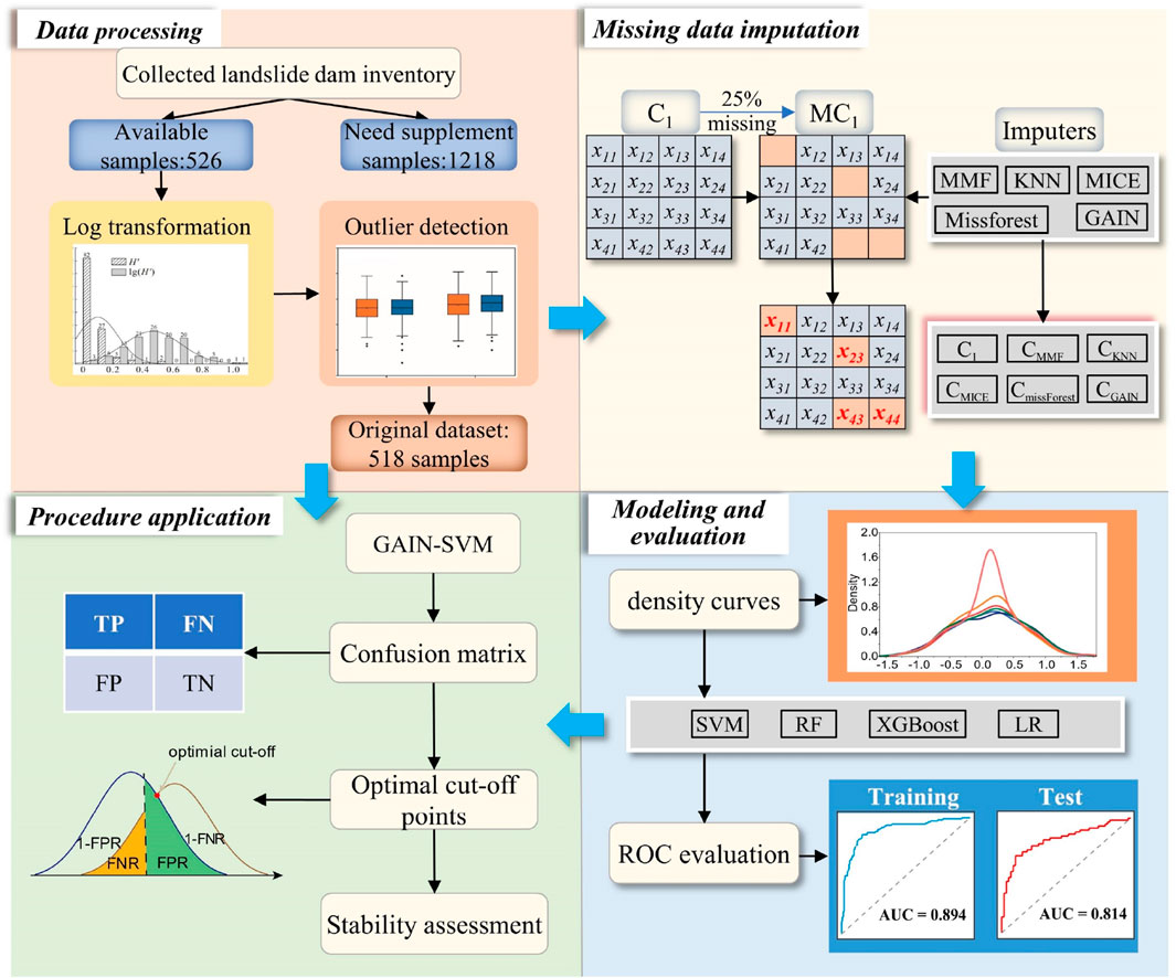
Figure 3. The framework for estimating the stability of landslide dams considering missing data imputation.

4 Results

4.1 Missing data imputation accuracy

The missing data imputation for the MC dataset (220 cases) was carried out by applying these five imputation approaches proposed in section 3.1 (MMF, KNN, MICE, missForest, GAIN). However, for both continuous and categorical variables included in the MC dataset, there are slight differences in the application of the different imputation approaches. For the GAIN and missForest methods, they can deal with mixed-type missing data, and the root mean squared error (RMSE) and proportion of correctly classified were used for error evaluation for continuous and categorical variables, respectively.

For continuous variables, RMSE was selected over MAE as the primary evaluation metric because it more severely penalizes large imputation errors - a critical consideration for landslide dam stability prediction, where extreme values of parameters like dam height or volume can disproportionately impact stability outcomes. While MAE provides a robust measure of average error magnitude, RMSE’s quadratic nature better reflects the operational reality that gross underestimations (e.g., of dam volume) could lead to catastrophic misjudgments in emergency scenarios. This aligns with standard practice in geotechnical risk assessment, where conservative error evaluation is preferred (Zhang et al., 2017). For completeness, both metrics were computed during development, but only RMSE results are reported as they more stringently differentiate imputation method performance.

For the MICE and KNN methods, the missing data imputation was first conducted on the category variable of M, and then the five continuous variables (V, H, L, W, A) were estimated. Finally, different imputation datasets were generated by the five imputation schemes. Figure 4 shows a comparison of the frequency or density curves for the imputed and observed datasets. It clearly shows that the density and frequency distributions between the imputed values for the missing data and observed values were similar for the four interpolation methods, except for the MMF method, which indicated that the interpolation results are valid. For MMF, all missing values for each variable were filled with the same value, thus showing a stronger concentration around the mean value. Furthermore, to compare the performance of the different imputation methods more intuitively, classification accuracy (ACC) and root mean square error (RMSE) were reported as evaluation metrics to measure the errors of the imputation results (Table 2). For the category variable, the MICE method outperformed the comparison imputers and produced the highest ACC value (70.2%). The following were the GAIN and missForest that had the same accuracy (66.0%), and the KNN and MMF ranked last among all methods with ACC values of 59.6% and 40.4%, respectively. Besides, for the imputation of continuous variables, the missForest had the best performance with the lowest RMSE value among the five imputers. The detailed order in the continuous variables is missForest > GAIN > MICE > KNN > MMF.

Figure 4

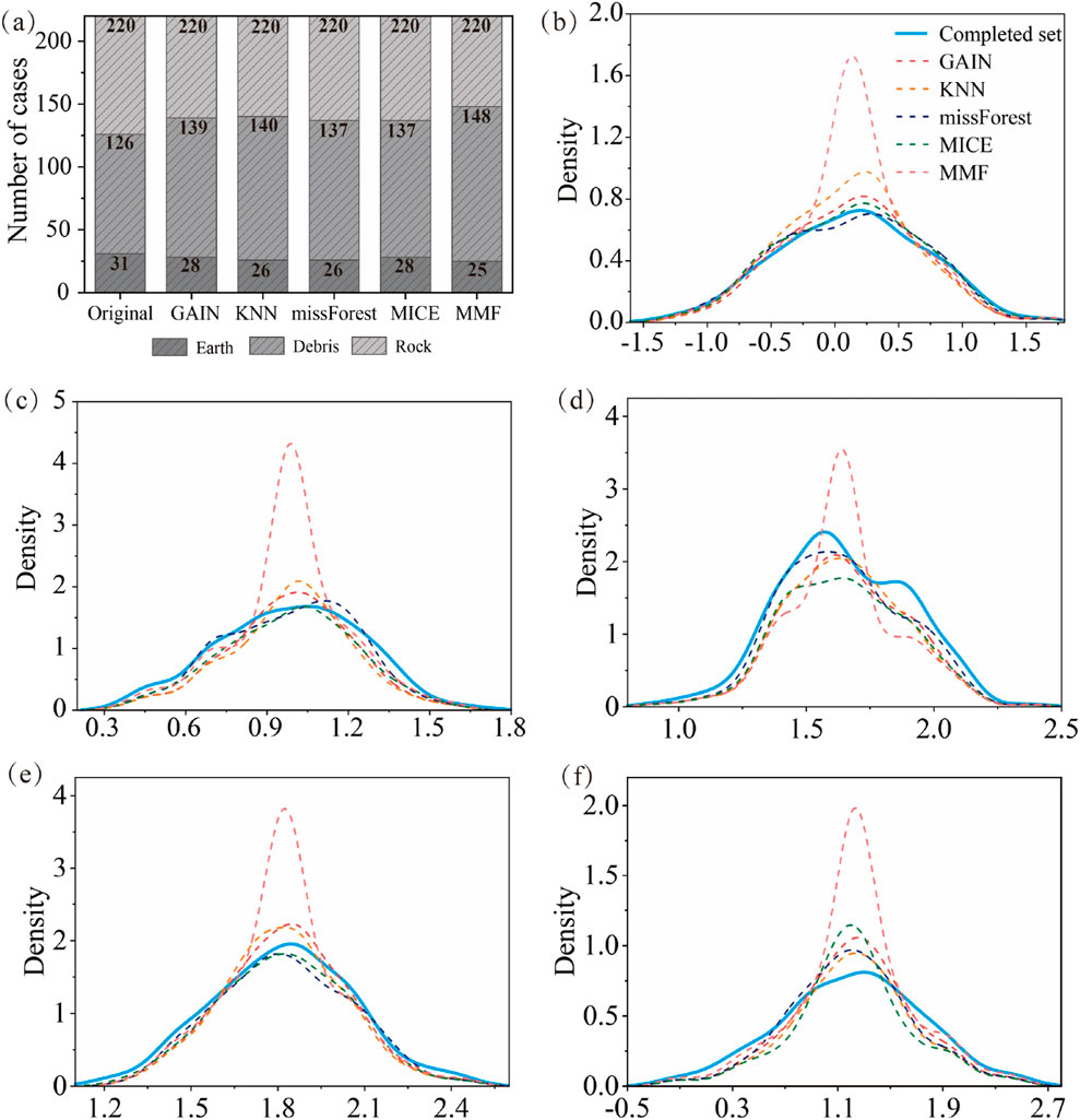
Figure 4. Comparison of frequency distribution or density curves of variables between complete data and five imputed datasets. (a) Material composition, (b) dam volume, (c) dam height, (d) dam length, (e) dam width, (f) catchment area.

Table 2

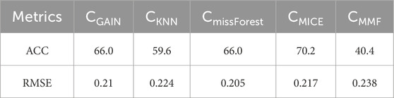
Table 2. Performance evaluation for different missing data imputation techniques.

4.2 Comparison of the predictive performance of different ML combined with imputation approaches

In this part, the landslide dam stability prediction experiments were conducted on the completed dataset (C₁) and five imputed datasets. All of these datasets have 220 completed landslide dam cases with the aim of validating the effectiveness of the proposed landslide dam stability prediction framework. In addition, to better quantitatively explain the rationality and performance of the SVM model, the other three commonly used machine learning approaches (RF, XGBoost and LR) were used for comparison.

4.2.1 Multicollinearity diagnosis

Before using these databases for the task of modeling the stability of landslide dams, a multicollinearity analysis is essential to delineate whether correlated variables exist among the variables. Indeed, considerable correlations between variables can reduce the predictive accuracy of ML models. The Variance Inflation Factor (VIF) was an effective statistics index that was used to check the multicollinearity relationships between landslide dam conditioning factors in this study (Curto and Pinto, 2010). Generally, VIF values range from 1 to 10, with a VIF greater than 10 indicating the presence of a notable multicollinearity problem. A VIF close to 1 refers to less multicollinearity. Figure 5 shows the VIF analysis the results of the VIF analysis for C₁ and the five computed datasets. It is obvious that all the conditioning variables in the six databases show similar multicollinearity relationships. Overall, the geometric variables (V, H, L, W) had higher values of VIF compared to the dam properties and hydrological variables (M and A). However, all the variables in the six databases had VIF values lower than 10, suggesting that there was no serious multicollinearity problem. Thus, all six variables in these six databases were accepted for modeling the stability of landslide dams.

Figure 5

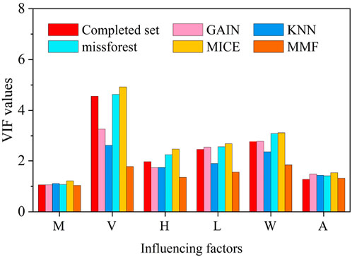
Figure 5. VIF test of the conditioning factors for six completed datasets.

4.2.2 Landslide dam stability prediction performance

The XGBoost, SVM, RF and LR algorithms were called from the Scikit-learn library in the Python environment for landslide dam stability modeling, and grid search and cross-validation techniques were used to optimize the hyper-parameters. These models calculated the probability of landslide dam stability on the completed dataset (C₁) and five imputed datasets in turn, which comprise a total of 24 modelling tests. Based on the test samples, which accounted for 30% of the total sample set, the ROC curves were produced to test each assessment result (Figure 6), from which the AUC values were calculated to quantify the prediction performance. It is to be noted that the values of the AUC values presented in Figure 6f were from ten test results, as obtained based on the 5-fold cross-validation.

Figure 6

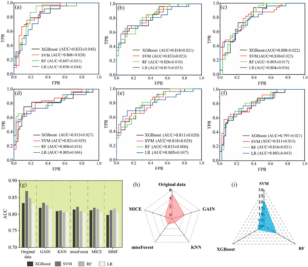
Figure 6. Prediction accuracies of ML models presented by ROC curves using the test sets for the six datasets. (a) Initial completed dataset (C₁), (b) GAIN imputed dataset, (c) KNN imputed dataset, (d) missForest dataset, (e) MICE imputed dataset, (f) MMF imputed dataset. (g) The AUC values for the 4 ML models on six datasets. (h) Improvement rate of overall AUC for different data sets compared to MMF. (i) Improvement rate of overall AUC for different MLs compared to LR.

The results of the six scenarios of various datasets suggested that the initial completed sample set-based assessments exhibited much better predictive effects with AUC values larger than 0.83 for all their prediction models. For the missing data imputation scenarios, each ML model was able to provide relatively good predictive results, since almost all models having AUC values greater than 0.8. However, compared to the initial complete dataset, the predictive performance of the four approaches for landslide dam stability modeling was slightly inferior after missing values imputation, with their overall AUC values reduced by 2.8% ∼ 4.8%. Among the five imputation approaches, the prediction performance on the GAIN imputed dataset was outperformance than other imputation techniques. The MMF and KNN approaches ranked last among all imputation approaches. In general, the ranking of ML predictive performance on different imputations was GAIN > MICE > missForest > KNN > MMF. Figure 6h compares the relative improvement ratios of the ML- (KNN, MICE, missForest) and DL-based (GAIN) imputation techniques to the statistically-based imputation method (MMF). The average relative improvement ratio of AUC between the GAIN and standard MMF was the highest reached at 2.11%. The relative improvement ratios of the KNN compared to MMF were far lower than those of the GAIN, missForest and MICE. These results indicated that the ML-based imputers, especially the DL-based imputation (GAIN), provide a better relative improvement than the statistically-based approaches of MMF. This is because DL methods focus on discovering complex decision rules and patterns from data for generalization and prediction. In contrast, traditional statistical methods emphasize explanation and inference to explore causal relationships behind observed phenomena. Hence, ML and DL techniques are often considered to have more flexible and predictive powers.

Consistent with Table 2’s imputation metrics, GAIN-SVM demonstrated the strongest predictive performance (AUC = 0.823, Figure 6f), a 15.2% improvement over baseline LR models. The ROC curves (Figures 6a–f) further validated that GAIN’s lower RMSE (Table 2) correlated with tighter confidence intervals and higher AUC values across all ML models. Specifically, the relative improvement ratios in Figure 6h mirrored the RMSE rankings from Table 2, with GAIN (2.11% gain over MMF) surpassing MICE (1.89%) and missForest (1.67%).

Furthermore, among the 4 ML modeling approaches, the SVM, RF and XGBoost showed better performance as compared to LR on most imputed datasets (Figure 6). The GAIN-SVM combination achieved the highest AUC (0.823), demonstrating a 15.2% improvement over LR (0.714) and 9.8% over MICE-RF (0.749). These quantified gains highlight its superiority for stability prediction. Furthermore, the RF showed robust performance with lower standard deviation, indicating that the RF had an excellent and robust performance in predicting the stability of landslide dams. Generally, SVM and LR models were more sensitive compared to RF and XGBoost models. The main reason is that SVM and LR models rely on support vectors or optimizing a decision boundary based on the proximity of points, which makes them sensitive to outliers. On the other hand, RF and XGBoost models tend to be relatively more robust to outliers since they are essentially ensemble algorithms that reduce volatility by constructing multiple decision trees (Webb and Zheng, 2004).

The Youden-index-based threshold optimization further enhanced accuracy by 3.1%–9.3% compared to the fixed 0.5 threshold (Table 3), particularly for cases with prediction probabilities near 0.5. This dual advancement, both imputation and classification-addresses critical limitations of traditional methods.

Table 3

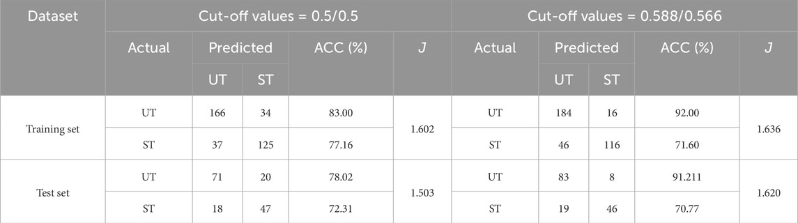
Table 3. Comparison of prediction accuracy between Youden and fixed-threshold methods in the training and test sets.

Overall, according to the statistics and ROC evaluation, the evaluation of landslide dam stability resulting from all the models showed a decent predictive performance towards the collected landslide dams. Among all the approaches, the performance of the GAIN imputation combined with the SVM model was better than the other approaches by 3.0 ∼ 13.5% for the objective of evaluating landslide dam stability with missing variables. This, therefore, suggests that it can be a powerful tool for assessing the landslide dam stability even when it contains missing values.

4.3 GAIN-SVM based stability prediction of landslide dams on MD set

In the section 4.2, the GAIN-SVM was considered the best combination for predicting the stability of landslide dams, from the perspective of ROC evaluation. Thus, GAIN was used to impute the missing values of the real landslide dam inventory with 518 cases (OM) and SVM was used to implement the modeling task.

4.3.1 Factor characteristics of the OM and GAIN imputed datasets

Figure 7 shows similar distributions for all six factors between original and GAIN-imputed datasets. Between these two datasets, the values for dam volume, dam height and dam length were larger for the ST landslide dams than those for the UT landslide dams, indicating that these three factors have a positive effect on the ST landslide dams. In contrast, the values for catchment area were lower for ST landslide dams than those for UT landslide dams. This indicates that the factor of catchment area factor was negatively correlated with the UT landslide dams. However, there were differences between the original and GAIN imputed datasets for the variable dam width. In the original data, the values of dam width for the ST landslide dams were smaller than those for the UT landslide dams, whereas the opposite was true in the GAIN imputed datasets. This result is consistent with the previous studies (Fan et al., 2020; Zheng et al., 2021). On the one side, the dam width can reflect the dams mass magnitude, and on the other side, the direction of the river flow is consistent with the direction of the dam width. Since, a larger value of dam width indicates that the difficulty of the river to damager is greater. Therefore, compared to the original dataset with missing information, the GAIN imputed dataset may contain more reasonable dam information.

Figure 7

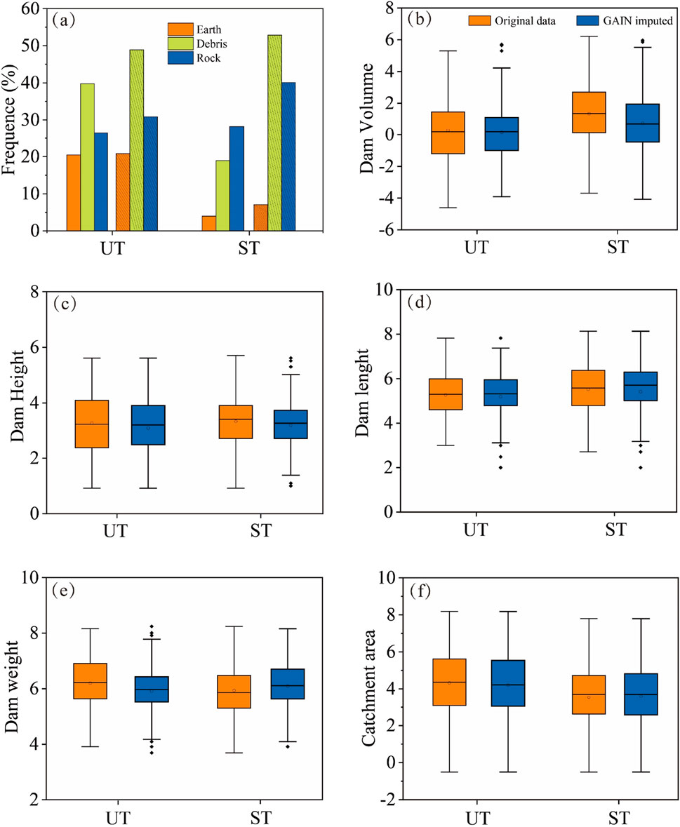
Figure 7. The influencing factors comparisons for ST and UT landslide dam on two datasets. (a) Material composition, chart with slashes lines indicates GAIN imputed set otherwise original set; (b) dam volume; (c) dam height; (d) dam length; (e) dam width; (f) catchment area. In the box-plot, the horizontal line defines the median, circle is the average value, the upper and lower limits of the box define the upper and lower quartiles (75% and 25% respectively), the whiskers are the minimum and maximum values, and the black diamonds are boxplot outliers.

4.3.2 GAIN-SVM prediction accuracy

After the GAIN imputed the missing values, the SVM approach was applied to perform the landslide dam stability modeling. It should be mentioned that in the all 518 landslide dam cases, the UT and ST cases are 291 and 227 respectively, the ratio is approximately 5:4. For the sample imbalance problem, unbalanced cost function weights were used to improve the impact of stable cases during model training. The weight ratio for unstable to stable cases was set to 4:5. In addition, multiple metrics based on the confusion matrix, including ROC curves, AUC, ACC, and the Youden index, can provide a reliable and comprehensive assessment for the GAIN-SVM model.

The quantitative evaluation of imputation methods (Table 2) revealed GAIN’s dual superiority: it achieved the lowest RMSE (0.205) for continuous variables and the second-highest accuracy (66.0%) for categorical data. This performance translated directly to predictive modeling, where GAIN-imputed data paired with SVM yielded the highest AUC (0.823, Figure 6f), outperforming other combinations by 3.0%–13.5%. Notably, the RMSE gap between GAIN and the next-best method (missForest, RMSE = 0.205 vs. 0.21) aligns with the AUC improvements observed in Figure 6h, demonstrating how imputation accuracy affects downstream prediction tasks.

First, the results of the relative contribution (RC) analysis of the conditioning factors for the SVM revealed the weighting of the causal factors (Figure 8a). The RC of the influencing factors can be ranked in the following order of decreasing importance: catchment area (RC = 0.28), landslide volume (RC = 0.22), material composition (RC = 0.17), dam height (RC = 0.15), dam length (RC = 0.10) and dam width (RC = 0.08). Overall, this probably indicates that the hydrological factors were more important than the dam geometric factors in modeling the stability of landslide dams. However, due to limitations in the available samples, the recorded data on hydrological factors were insufficient, such as the values of average annual flow and peak flow, both of which contained missing values exceeding 80%. In this study, only the catchment area was used in the SVM for describing the hydrological effect.

Figure 8

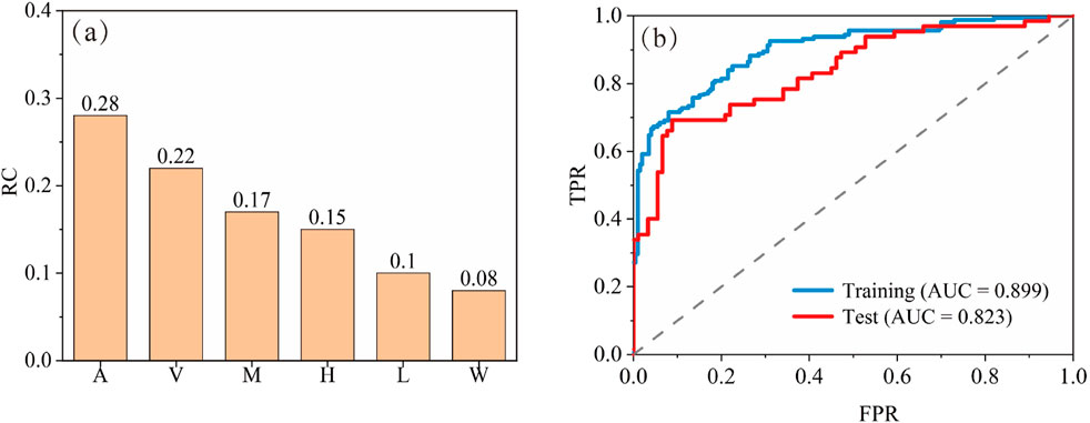
Figure 8. Evaluation of the GAIN-SVM model. (a) Variables relative contribution calculated from SVM, (b) ROC curves based on training and test dataset.

Second, ROC curves and the AUCs were calculated to evaluate the performance of the trained GAIN-SVM model on two different datasets, training and test sets respectively, which aims to estimate the fitting and prediction accuracy of the GAIN-SVM (Figure 8b). The calculation results showed that the GAIN-SVM had a decent fitting and predicting performance with the AUCs of 0.899 and 0.823, respectively. The value of the AUC obtained on the test dataset displayed slightly smaller patterns, but was comparable to those obtained on the training dataset. The reason for this can be attributed to the fact that the supervised learning process was used for the latter, whereas the former modelling process was predominantly unsupervised.

Third, based on the ROC curves, we further calculated the optimal cut-off point to recognize the ST and UT landslide dams. These optimal classification thresholds for the training and test sets were 0.588 and 0.566, respectively. The classification results showed high accuracy for both stability states: 92.00% for UT and 71.60% for ST in training, and 91.21% (UT) vs. 70.77% (ST) in testing. This demonstrates robust discrimination of stability states despite imputed data. For these two datasets, the total ACCs values were 82.87% and 82.69%. Besides, table 3 shows the comparison for the statistical results between Youden method with the traditional method which used a fixed threshold of 0.5 to classify the UT and ST landslide dams. In training and test sets, the ACC based on Youden method was improved by 3.09% and 9.32% respectively compared to the traditional discrimination method. In addition, the higher Youden index indicates the higher value of TPR or lower value of FPR. Although the numerical performance in terms of accuracy improvement was not significant, the cases of misclassification were commonly very close to the threshold point and difficult to identify. Thus, even a small increase in accuracy can lead to a large change in the optimal threshold point.

5 Discussion

5.1 Verification of missing data imputation using common rapid evaluation methods

In order to further verify the application of the imputation approach in the landslide dam stability prediction task, two commonly used rapid evaluation methods including DBI and L_s (AHWL) (Ermini and Casagli, 2003; Dong et al., 2011) were introduced to the C₁ and GAIN imputed OM databases. Because the required parameters of these two methods were included in the six imputed factors, including five geometries and one hydrological factor. On the two datasets, the C₁ contained only 220 complete cases with no missing values, while the other set imputed all missing values and generated a total of 518 landslide dam cases. As table 4 shows, the two kinds of rapid evaluation methods, DBI and L_s (AHWL), have reported similar accuracy no matters on completed cases and imputed cases. To be exact, compared with the GAIN imputed set, the performance of DBI and AHWL were slightly outperform by 5.06% and 0.106% on the C₁ set.

Table 4

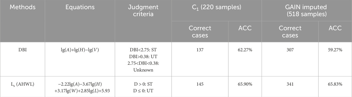
Table 4. Prediction accuracy of different rapid landslide dam stability evaluation methods on completed and GAIN imputed sets.

The slight accuracy difference (5.06% for DBI) between original and imputed data arises because observed stability states (ST/UT) reflect ground truth, while imputed values approximate missing parameters. Nevertheless, the GAIN-imputed dataset expanded usable cases by 2.35× with minimal accuracy trade-off. Nevertheless, compared to the slight loss in performance, the improvement in terms of the application of these rapid evaluation methods is significant, since the number of available cases after missing value filling is 2.35 times the number of originally completed cases. In areas prone to landslide dam formation, such as high mountain valleys, it is difficult to accurately measure all the required relevant parameters due to topographical constraints, which can limit the application of traditional rapid assessment methods. The GAIN-based missing data extrapolation method proposed in this study can generate reasonable imputation values from observed variables and contribute to the application of various rapid assessment methods for the initial assessment of landslide dam stability.

5.2 The influence of missing rate on modeling accuracy tested on C₁ set

Based on the collected landslide dam inventory, we discussed the appropriate missing data imputation technique and ML modeling for the landslide dam stability prediction. But considering the different data available, different data missing rates and missing pattern may occur. In this part, different missing rates are discussed based on the framework of GAIN-SVM. Besides, the latest landslide dam stability approach based on XGBoost (Shi et al., 2022), which has effective missing data processing ability and well prediction accuracy will be introduced for competition.

For missing rates of 5%–50%, Figure 9 compares test-set AUC values of GAIN-SVM, GAIN-XGBoost, and XGBoost-only models. It is clear that all three models illustrate a decrease in prediction accuracy as the missing rate increases, but with different patterns. The GAIN-SVM exhibit a slight decrease in performance when the missing rate is below 40%, but once the missing rate rises above 40%, the loss in performance is severe. Whereas, for GAIN-XGBoost and XGBoost only, the decline in AUC starts to accelerate as the missing rate is greater than 20%, and when the missing rate reaches 50%, the prediction accuracy drops to 0.653 and 0.673 respectively. Among these three prediction methods, the performance of GAIN imputer combined with SVM was outperformed than GAIN-XGBoost and only XGBoost approaches. Specifically, the AUC values can be improved by 3.65%∼12.25% compared to the other models. For the XGBoost model, which has a built-in handling procedure for missing values, the use of missing data imputation technique (GAIN-XGBoost) did not improve the prediction accuracy compared to the XGBoost only model. In particular, the Wilcoxon Rank Sum Test showed that there was not a significant difference in performance between XGBoost and GAIN-XGBoost (p > 0.05).

Figure 9

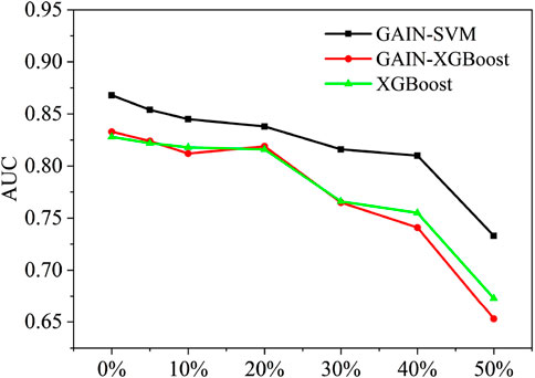
Figure 9. AUC performance in different missing rate settings on C₁ dataset.

All models exhibited declining accuracy for missing rates >40%, but GAIN-SVM maintained superior discrimination of stability states (ST/UT), with AUC drops of 15.55% vs. 21.60% for GAIN-XGBoost. The prediction accuracy of AUC values decreased by 15.55%, 21.60% and 18.71% respectively. This is since as the information contained in the observed data decreases, the difficulty and uncertainty of imputing missing values increases significantly. Hence, the results of this study suggest that the proposed GAIN-SVM can perform the landslide dam stability prediction as the total missing rate is lower than 40%.

For landslide dam datasets with >40% missing values, we recommend two hybrid approaches that integrate physical models with data-driven methods: (1) Physics-constrained imputation using sediment transport equations to estimate missing geomorphic parameters (Argentin et al., 2021); (2) Satellite-based reconstruction of dam dimensions from topographic data (Fan et al., 2020). These methods have demonstrated success in handling 50%–60% missing rates while maintaining physical plausibility, as evidenced by their applications to real landslide dam cases in peer-reviewed studies.

5.3 The relationship between missing pattern and landslide dam stability

In this part, we discussed the relationship between the occurrence of missing values and the stability of landslide dams. Besides, we proposed a ratio index (RI), which was obtained by divided the percentage of the missing values for each variable by the percentage of the cases in the two types of stability states (UT and ST). The RI value larger than 1 means that the landslide dam stability state is positively correlated with the occurrence of missing values, whereas the RI lower than 1 indicates the landslide dam stability state is negatively correlated with occurrence of missing values. The final calculated RI results for each variable were shown in Figure 10. We can see that the material composition (M) and landslide dam volume (V) were more easily to be lost when investigation and recording for the ST landslide dam. On the contrary, the values of variables that were more likely to be lost for UT landslide dams were dam height (H), dam length (L) and catchment area (A). As for dam width (W), the relationship between the missing data and the stability state of the dam is not significant. In fact, common patterns of missing landslide dam inventory are categorized into three types based on the relationship between the missing and the observed values (Emmanuel et al., 2021):

(1) Missing Completely at Random (MCAR): MCAR occurs when the missingness is completely independent of all the variables present in the data. For example, a variable that a researcher might accidentally overlook in a survey.

(2) Missing at Random (MAR): The MAR mechanism supposes the missingness is related to only the observed variables. As show in Figure 10, the landslide dam material composition has higher missing possible for the ST landslide dam.

(3) Missing Not at Random (MNAR): MNAR exists when the missingness is dependent on both the observed and missing variables.

Figure 10

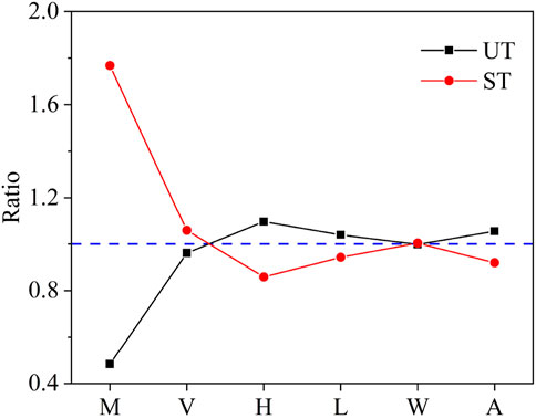
Figure 10. RI values for different variables in UT and ST landslide dam cases.

Missing data patterns in landslide dam inventories reflect both data-collection challenges and inconsistent recording standards, creating mixed missing patterns (MMMP). In the two group experiments (MCAR refers to MC, MMMP corresponds to OC), the difference in the missing pattern may be responsible for the performance variation in performance of the GAIN-SVM models between the MAR dataset and the real-word dataset (Wang and Wang, 2009; Halder et al., 2021). Thus, there is still a need to explore the patterns of missingness in dam datasets, which may contribute to identify new potential relationships between the stability of landslide dams and the factors of interest.

Geographic analysis revealed spatial performance patterns, with the framework achieving 89.2% accuracy for earthquake-triggered dams (e.g., 2008 Wenchuan cases, n = 37) versus 74.6% for rainfall-induced dams. This disparity likely stems from more consistent material properties and failure modes in seismic events (Chen et al., 2014), enhancing imputation reliability. Such regional variations highlight the value of context-specific calibration when applying the method globally.

6 Conclusion

The current landslide dam database generally contains a large amount of missing data, which has been limited the application of data-driven models in landslide dam stability prediction, including machine learning methods and statistical methods. In the current study, a novel landslide dam stability assessment framework was proposed that can account for the missing values in the dataset. Compared with previous studies, the contributions of this study mainly include two aspects: (i) the missing value imputation has extended the application of data-driven models to real dam datasets, and (ii) the optimal classification threshold based on Youden index and ROC analysis has been adopted to improve the discrimination accuracy of the models. Based on the experiences obtained from a total of 518 landslide dam cases with approximately 25% missing values, we stated that compared with the prediction accuracy of the completed cases, the prediction accuracy after imputation of missing values had decreased by 2.8%–4.8%, but the overall accuracy was still exceed 80%, which was considered acceptable, and the number of cases available for stability evaluation increased by a factor of 2.35. Specifically, a total of 24 experiments contained the four machine learning methods (XGBoost, SVM, RF, LR) performing landslide dam stability assessment on five imputed databases (GAIN, KNN, missForest, MICE and MMF) and one complete dataset. The results show that the GAIN combined with SVM has higher prediction accuracy in these competitions. Furthermore, compared with the fixed threshold discriminant method, the Youden index discriminant can improve the prediction accuracy by 3.09 ∼ 9.32%, which can also assist users to further improve the prediction accuracy of ML-based methods for existing landslide dam stability evaluation. Depending on the test results from different missing rates, the proposed procedure can achieve relatively robust performance with the missing rate lower than 40%. While accuracy declines with missing rates >40%, the framework remains viable for most practical scenarios, expanding usable cases by 2.35× compared to complete-data approaches.

By enabling reliable stability predictions with incomplete field data, this framework supports rapid prioritization of high-risk dams during emergencies, empowering authorities to allocate mitigation resources efficiently. Its integration into early warning systems could enhance community resilience in landslide-prone regions, reducing downstream infrastructure losses and saving lives.

Data availability statement

The original contributions presented in the study are included in the article/supplementary material, further inquiries can be directed to the corresponding author.

Author contributions

XL: Methodology, Writing – original draft, Software. XZ: Writing – review and editing, Formal Analysis. JH: Conceptualization, Writing – review and editing. YS: Supervision, Writing – review and editing, Data curation. YL: Validation, Writing – review and editing.

Funding

The author(s) declare that financial support was received for the research and/or publication of this article. The research was supported by the National Natural Science Foundation of China (Nos. 42272331, 41902290) and by Natural Science Foundation of Hebei Province (No. D2020202002).

Conflict of interest

The authors declare that the research was conducted in the absence of any commercial or financial relationships that could be construed as a potential conflict of interest.

Generative AI statement

The author(s) declare that no Generative AI was used in the creation of this manuscript.

Publisher’s note

All claims expressed in this article are solely those of the authors and do not necessarily represent those of their affiliated organizations, or those of the publisher, the editors and the reviewers. Any product that may be evaluated in this article, or claim that may be made by its manufacturer, is not guaranteed or endorsed by the publisher.

References

Argentin, A.-L., Robl, J., Prasicek, G., Hergarten, S., Hölbling, D., Abad, L., et al. (2021). Controls on the formation and size of potential landslide dams and dammed lakes in the Austrian Alps. Nat. Hazards Earth Syst. Sci. 21, 1615–1637. doi:10.5194/nhess-21-1615-2021

CrossRef Full Text | Google Scholar

Arriagada, P., Karelovic, B., and Link, O. (2021). Automatic gap-filling of daily streamflow time series in data-scarce regions using a machine learning algorithm. J. Hydrology 598, 126454. doi:10.1016/j.jhydrol.2021.126454

CrossRef Full Text | Google Scholar

Awan, S. E., Bennamoun, M., Sohel, F., Sanfilippo, F., and Dwivedi, G. (2021). Imputation of missing data with class imbalance using conditional generative adversarial networks. Neurocomputing 453, 164–171. doi:10.1016/j.neucom.2021.04.010

CrossRef Full Text | Google Scholar

Buuren, S. v., and Groothuis-Oudshoorn, K. (2011). Mice: multivariate imputation by chained equations in R. J. Stat. Softw. 45, 1–67. doi:10.18637/jss.v045.i03

CrossRef Full Text | Google Scholar

Chen, C.-Y., and Chang, J.-M. (2015). Landslide dam formation susceptibility analysis based on geomorphic features. Landslides 13, 1019–1033. doi:10.1007/s10346-015-0671-5

CrossRef Full Text | Google Scholar

Chen, K.-T., Kuo, Y.-S., and Shieh, C.-L. (2014). Rapid geometry analysis for earthquake-induced and rainfall-induced landslide dams in Taiwan. J. Mt. Sci. 11, 360–370. doi:10.1007/s11629-013-2664-y

CrossRef Full Text | Google Scholar

Cortes, C., and Vapnik, V. (1995). Support-vector networks. Mach. Learn. 20, 273–297. doi:10.1007/bf00994018

CrossRef Full Text | Google Scholar

Costa, J. E., and Schuster, R. L. (1991). Documented historical landslide dams from around the world. U. S. Geol. Surv. Open-file Rep., 91–239. doi:10.3133/ofr91239

CrossRef Full Text | Google Scholar

Curto, J. D., and Pinto, J. C. (2010). The corrected VIF (CVIF). J. Appl. Statistics 38, 1499–1507. doi:10.1080/02664763.2010.505956

CrossRef Full Text | Google Scholar

Dong, J.-J., Tung, Y.-H., Chen, C.-C., Liao, J.-J., and Pan, Y.-W. (2011). Logistic regression model for predicting the failure probability of a landslide dam. Eng. Geol. 117, 52–61. doi:10.1016/j.enggeo.2010.10.004

CrossRef Full Text | Google Scholar

Ehteshami-Moinabadi, M., and Nasiri, S. (2017). Geometrical and structural setting of landslide dams of the Central Alborz: a link between earthquakes and landslide damming. Bull. Eng. Geol. Environ. 78, 69–88. doi:10.1007/s10064-017-1021-8

CrossRef Full Text | Google Scholar

Emmanuel, T., Maupong, T., Mpoeleng, D., Semong, T., Mphago, B., and Tabona, O. (2021). A survey on missing data in machine learning. J. Big Data 8, 140. doi:10.1186/s40537-021-00516-9

PubMed Abstract | CrossRef Full Text | Google Scholar

Ermini, L., and Casagli, N. (2003). Prediction of the behaviour of landslide dams using a geomorphological dimensionless index. Earth Surf. Process. Landforms 28, 31–47. doi:10.1002/esp.424

CrossRef Full Text | Google Scholar

Fan, X., Dufresne, A., Subramanian, S. S., Strom, A., Hermanns, R., Kenneth, A., et al. (2020). The formation and impact of landslide dams - state of the art. Earth-Science Rev. Int. Geol. J. Bridg. Gap between Res. Articles Textb. 203, 103116. doi:10.1016/j.earscirev.2020.103116

CrossRef Full Text | Google Scholar

Fan, X., Rossiter, D. G., van Westen, C. J., Xu, Q., and Görüm, T. (2014). Empirical prediction of coseismic landslide dam formation. Earth Surf. Process. Landforms 39, 1913–1926. doi:10.1002/esp.3585

CrossRef Full Text | Google Scholar

Fawcett, T. (2006). An introduction to ROC analysis. Pattern Recognit. Lett. 27, 861–874. doi:10.1016/j.patrec.2005.10.010

CrossRef Full Text | Google Scholar

Feng, R., Grana, D., and Balling, N. (2021). Imputation of missing well log data by random forest and its uncertainty analysis. Comput. and Geosciences 152, 104763. doi:10.1016/j.cageo.2021.104763

CrossRef Full Text | Google Scholar

Frigerio Porta, G., Bebbington, M., Xiao, X., and Jones, G. (2020). Bayesian lifetime analysis for landslide dams. Landslides 17, 1835–1848. doi:10.1007/s10346-020-01388-5

CrossRef Full Text | Google Scholar

Halder, B., Ahmed, M. M., Amagasa, T., Isa, N. A. M., Faisal, R. H., and Rahman, M. M. (2021). Missing information in imbalanced data stream: fuzzy adaptive imputation approach. Appl. Intell. 52, 5561–5583. doi:10.1007/s10489-021-02741-4

CrossRef Full Text | Google Scholar

Jin, J., Chen, G., Meng, X., Zhang, Y., Shi, W., Li, Y., et al. (2022). Prediction of river damming susceptibility by landslides based on a logistic regression model and InSAR techniques: a case study of the Bailong River Basin, China. Eng. Geol. 299, 106562. doi:10.1016/j.enggeo.2022.106562

CrossRef Full Text | Google Scholar

Jung, C., Lee, Y., Lee, J., and Kim, S. (2020). Performance evaluation of the multiple quantile regression model for estimating spatial soil moisture after filtering soil moisture outliers. Remote Sens. 12, 1678. doi:10.3390/rs12101678

CrossRef Full Text | Google Scholar

Korup, O. (2004). Geomorphometric characteristics of New Zealand landslide dams. Eng. Geol. 73, 13–35. doi:10.1016/j.enggeo.2003.11.003

CrossRef Full Text | Google Scholar

Li, D., Nian, T., Wu, H., Wang, F., and Zheng, L. (2020). A predictive model for the geometry of landslide dams in V-shaped valleys. Bull. Eng. Geol. Environ. 79, 4595–4608. doi:10.1007/s10064-020-01828-5

CrossRef Full Text | Google Scholar

Liao, H.-m., Yang, X.-g., Lu, G.-d., Tao, J., and Zhou, J.-w. (2022). A geotechnical index for landslide dam stability assessment. Geomatics, Nat. Hazards Risk 13, 854–876. doi:10.1080/19475705.2022.2048906

CrossRef Full Text | Google Scholar

Liao, H.-m., Yang, X.-g., Xu, F.-g., Xu, H., and Zhou, J.-w. (2018). A fuzzy comprehensive method for the risk assessment of a landslide-dammed lake. Environ. Earth Sci. 77, 750. doi:10.1007/s12665-018-7946-9

CrossRef Full Text | Google Scholar

Lin, W.-C., Tsai, C.-F., and Zhong, J. R. (2022). Deep learning for missing value imputation of continuous data and the effect of data discretization. Knowledge-Based Syst. 239, 108079. doi:10.1016/j.knosys.2021.108079

CrossRef Full Text | Google Scholar

Lobato, F., Sales, C., Araujo, I., Tadaiesky, V., Dias, L., Ramos, L., et al. (2015). Multi-objective genetic algorithm for missing data imputation. Pattern Recognit. Lett. 68, 126–131. doi:10.1016/j.patrec.2015.08.023

CrossRef Full Text | Google Scholar

Lyngdoh, G. A., Zaki, M., Krishnan, N. M. A., and Das, S. (2022). Prediction of concrete strengths enabled by missing data imputation and interpretable machine learning. Cem. Concr. Compos. 128, 104414. doi:10.1016/j.cemconcomp.2022.104414

CrossRef Full Text | Google Scholar

Mei, S., Chen, S., Zhong, Q., and Shan, Y. (2021). Effects of grain size distribution on landslide dam breaching—insights from recent cases in China. Front. Earth Sci. 9. doi:10.3389/feart.2021.658578

CrossRef Full Text | Google Scholar

Mohammadi, H., Hosseini, S. T., Asghari, O., Silva, C. Z. d., and Boisvert, J. B. (2021). A direct sampling multiple point statistical approach for multivariate imputation of unequally sampled compositional variables and categorical data. Comput. Geosciences 156, 104911. doi:10.1016/j.cageo.2021.104911

CrossRef Full Text | Google Scholar

Monica, L.-R., Marıa, X.R.-A., Carmen, C.-S., and Francisco, G.-S. (2014). OptimalCutpoints: an R package for selecting optimal cutpoints in diagnostic tests. J. Stat. Softw. 61. doi:10.18637/jss.v061.i08

CrossRef Full Text | Google Scholar

Nahm, F. S. (2022). Receiver operating characteristic curve: overview and practical use for clinicians. Korean J. Anesthesiol. 75, 25–36. doi:10.4097/kja.21209

PubMed Abstract | CrossRef Full Text | Google Scholar

Nian, T., Li, D., Liang, Q., Wu, H., and Guo, X. (2021). Multi-phase flow simulation of landslide dam formation process based on extended coupled DEM-CFD method. Comput. Geotechnics 140, 104438. doi:10.1016/j.compgeo.2021.104438

CrossRef Full Text | Google Scholar

Peng, M., Zhang, L., and Chang, D. (2016). Dam failure mechanisms and risk assessment. John Wiley and Sons.

Google Scholar

Qi, C., Fourie, A., Du, X., and Tang, X. (2018). Prediction of open stope hangingwall stability using random forests. Nat. Hazards 92, 1179–1197. doi:10.1007/s11069-018-3246-7

CrossRef Full Text | Google Scholar

Shan, Y., Chen, S., and Zhong, Q. (2020). Rapid prediction of landslide dam stability using the logistic regression method. Landslides 17, 2931–2956. doi:10.1007/s10346-020-01414-6

CrossRef Full Text | Google Scholar

Shen, D., Shi, Z., Peng, M., Zhang, L., and Jiang, M. (2020). Longevity analysis of landslide dams. Landslides 17, 1797–1821. doi:10.1007/s10346-020-01386-7

CrossRef Full Text | Google Scholar

Shi, N., Li, Y., Wen, L., and Zhang, Y. (2022). Rapid prediction of landslide dam stability considering the missing data using XGBoost algorithm. Landslides 19, 2951–2963. doi:10.1007/s10346-022-01947-y

CrossRef Full Text | Google Scholar

Sica, S., Pagano, L., and Rotili, F. (2019). Rapid drawdown on earth dam stability after a strong earthquake. Comput. Geotechnics 116, 103187. doi:10.1016/j.compgeo.2019.103187

CrossRef Full Text | Google Scholar

Song, Y., Zhang, X., and Huang, D. (2022). Stability prediction of landslide dams based on SSA-Adam-BP neural network model. Bull. Geol. Sci. Technol. 41, 130–138. doi:10.19509/j.cnki.dzkq.2022.0040

CrossRef Full Text | Google Scholar

Stefanelli, C. T., Catani, F., and Casagli, N. (2015). Geomorphological investigations on landslide dams. Geoenvironmental Disasters 2 (1), 21. doi:10.1186/s40677-015-0030-9

CrossRef Full Text | Google Scholar

Stefanelli, C. T., Vilímek, V., Emmer, A., and Catani, F. (2018). Morphological analysis and features of the landslide dams in the Cordillera Blanca, Peru. Landslides 15, 507–521. doi:10.1007/s10346-017-0888-6

CrossRef Full Text | Google Scholar

Stekhoven, D. J., and Buhlmann, P. (2012). MissForest--non-parametric missing value imputation for mixed-type data. Bioinformatics 28, 112–118. doi:10.1093/bioinformatics/btr597

PubMed Abstract | CrossRef Full Text | Google Scholar

Strom, A. (2013). Geological prerequisites for landslide dams’ disaster assessment and mitigation in central asia. Prog. Geo-Disaster Mitig. Technol. Asia, 17–53. doi:10.1007/978-3-642-29107-4_2

CrossRef Full Text | Google Scholar

Sun, Y., Li, J., Xu, Y., Zhang, T., and Wang, X. (2023). Deep learning versus conventional methods for missing data imputation: a review and comparative study. Expert Syst. Appl. 227, 120201. doi:10.1016/j.eswa.2023.120201

CrossRef Full Text | Google Scholar

Tabata, S., Mizuyama, T., and Inoue, K. (2002). Natural landslide dams hazards. Eng. Geol. 110 (3), 162–171. doi:10.1016/S0013-7952(02)00198-X

CrossRef Full Text | Google Scholar

Tacconi Stefanelli, C., Segoni, S., Casagli, N., and Catani, F. (2016). Geomorphic indexing of landslide dams evolution. Eng. Geol. 208, 1–10. doi:10.1016/j.enggeo.2016.04.024

CrossRef Full Text | Google Scholar

Tang, R., Fan, X., Scaringi, G., Xu, Q., van Westen, C. J., Ren, J., et al. (2018). Distinctive controls on the distribution of river-damming and non-damming landslides induced by the 2008 Wenchuan earthquake. Bull. Eng. Geol. Environ. 78, 4075–4093. doi:10.1007/s10064-018-1381-8

CrossRef Full Text | Google Scholar

Tang, X., Chen, A., and He, J. (2023). Optimized variable selection of Bayesian network for dam risk analysis: a case study of earth dams in the United States. J. Hydrology 617, 129091. doi:10.1016/j.jhydrol.2023.129091

CrossRef Full Text | Google Scholar

Wang, G., Huang, R., Kamai, T., and Zhang, F. (2013). The internal structure of a rockslide dam induced by the 2008 Wenchuan (Mw7.9) earthquake, China. Eng. Geol. 156, 28–36. doi:10.1016/j.enggeo.2013.01.004

CrossRef Full Text | Google Scholar

Wang, H., and Wang, S. (2009). Discovering patterns of missing data in survey databases: an application of rough sets. Expert Syst. Appl. 36, 6256–6260. doi:10.1016/j.eswa.2008.07.010

CrossRef Full Text | Google Scholar

Wang, S.-y., and Liu, J. (2013). Modeling the risk assessment of landslide-dammed lakes based on the emergency response measures in Wenchuan earthquake, 2008, China. Nat. Hazards 67, 523–547. doi:10.1007/s11069-013-0584-3

CrossRef Full Text | Google Scholar

Wang, X. a., Chen, J., Chen, H., Chen, X., Li, S., and Zhao, W. (2022). Erosion process of multiple debris flow surges caused by check dam removal: an experimental study. Water Resour. Res. 58. doi:10.1029/2021wr030688

CrossRef Full Text | Google Scholar

Webb, G., and Zheng, Z. (2004). Multistrategy ensemble learning: reducing error by combining ensemble learning techniques. IEEE Trans. Knowl. Data Eng. 16, 980–991. doi:10.1109/tkde.2004.29

CrossRef Full Text | Google Scholar

Yin, J., and Tian, L. (2014). Joint inference about sensitivity and specificity at the optimal cut-off point associated with Youden index. Comput. Statistics and Data Analysis 77, 1–13. doi:10.1016/j.csda.2014.01.021

CrossRef Full Text | Google Scholar

Yoon, J., Jordon, J., and Schaar, M. v.d. (2018). “GAIN: missing data imputation using generative adversarial nets,” in Proceedings of the 35th International Conference on Machine Learning, 5689–5698.

Google Scholar

Zhang, S., Li, X., Zong, M., Zhu, X., and Cheng, D. (2017). Learning k for kNN Classification. ACM Trans. Intelligent Syst. Technol. 8, 1–19. doi:10.1145/2990508

CrossRef Full Text | Google Scholar

Zhao, B., Wang, Y. S., Luo, Y. H., Li, J., Zhang, X., and Shen, T. (2018). Landslides and dam damage resulting from the Jiuzhaigou earthquake (8 August 2017), Sichuan, China. R. Soc. Open Sci. 5, 171418. doi:10.1098/rsos.171418

PubMed Abstract | CrossRef Full Text | Google Scholar

Zheng, H., Shi, Z., Shen, D., Peng, M., Hanley, K. J., Ma, C., et al. (2021). Recent advances in stability and failure mechanisms of landslide dams. Front. Earth Sci. 9. doi:10.3389/feart.2021.659935

CrossRef Full Text | Google Scholar