Volume changes at Santiaguito volcano between 2011 and 2019 based on TanDEM-X InSAR data

The Santiaguito volcanic dome complex in Guatemala consists of four volcanic domes formed within the 1902 eruption crater of Santa María volcano, with only the oldest dome, Caliente, currently active. Caliente is characterized by frequent explosive eruptions, rockfalls, pyroclastic flows, and blocky lava flows. TanDEM-X data enable the generation of high-resolution digital elevation models of complex volcanic terrain. Repeated acquisitions over the same area allow for the detection and quantification of topographic changes associated with volcanic activity. This study investigates elevation and volume changes at Caliente’s southern flank and western crater region from September 2011 to April 2019 using 24 TanDEM-X-derived digital elevation models with spatial resolutions of 6.5 m (N–S) and 4 m (E–W). Between 2011 and 2016, several new lava flows were emplaced on the southern flank, while the crater region experienced a volume decrease of $(545\pm 4)\cdot 10^3$ ${\text{m}}^3$. From 2016 to 2019, significant dome growth increased the volume in the crater region again by $(354\pm 3)\cdot 10^3$ ${\text{m}}^3$, primarily in the center. Concurrently, volume decreased along the northwestern crater rim, likely due to the 2016 explosive eruption. The average volume output rate over the entire observation period is calculated as $0.18\pm 0.0004$ ${\text{m}}^3$/s. The results align with previously determined cyclic patterns at Santiaguito volcano and provide a qualitative and quantitative description of the behavioral shift during our period of observation.

1 Introduction

The Santiaguito volcanic dome complex is located 11 km southwest of Quetzaltenango, Guatemala’s second-largest city. It formed within a 1,000 m $\times$ 700 m eruption crater on the southeastern flank of Santa María volcano, created during its 1902 Plinian event (Eisen, 1903; Stoiber and Rose, 1969; Rose, 1973; Williams and Self, 1983; Gottschämmer et al., 2021). Santiaguito has been growing continuously since volcanic activity resumed in 1922, approximately 20 years after the Santa María eruption. Over time, the westward-growing dome complex has developed four distinct domes: Caliente (1922–1939), La Mitad (1939–1949), El Monje (1949–1958), and El Brujo (1958–1986) in several growth spurts (Stoiber and Rose, 1969; Rose, 1972a; Rose, 1973; Harris et al., 2003; Scott, 2013). Figure 1 shows the geographical location of the Santiaguito volcanic dome complex. Over the last decades, activity at Santiaguito has included ash eruptions, pyroclastic flows, lava discharge, and fumarolic activity (Stoiber and Rose, 1969; Global Volcanism Program, 2025).

Figure 1

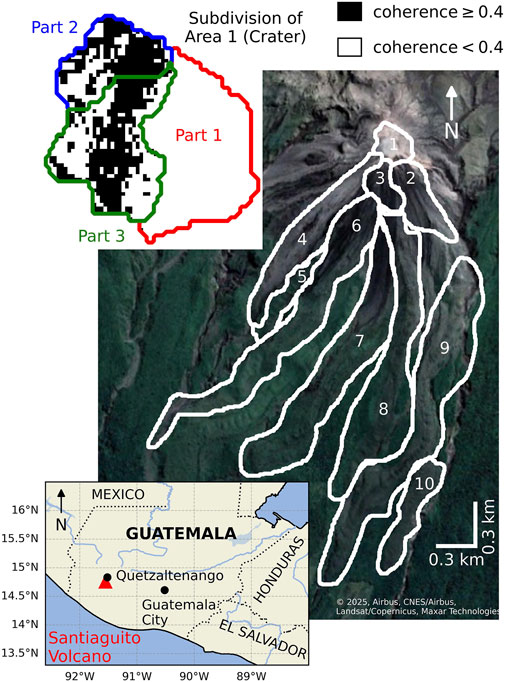
Figure 1. Definition of 10 areas to individually investigate spatio-temporal variations at Santiaguito volcano. Background image taken from Google Earth ©2025, Airbus, CNES/Airbus, Landsat/Copernicus, Maxar Technologies. The top left figure shows an additional subdivision of the crater region (Area 1) into 3 parts and the coherence in the crater region with black indicating sufficient coherence $\ge 0.4$. The coherence was extracted from the descending orbit DEMs only as these were the ones used for analysis of Area 1 as motivated in Section 2.5.2. The location of Santiaguito volcano in Guatemala, close to Quetzaltenango, is illustrated in the bottom left figure. The map was generated using the Python package Cartopy (Met Office, 2010).

Several studies have analyzed Santiaguito’s lava discharge and corresponding discharge rates (e.g., Rose et al., 1970; Rose, 1987; Harris et al., 2003; Ebmeier et al., 2012; Massaro et al., 2022), as understanding volume changes provides insight into both short- and long-term volcanic behavior. These analyses help constrain, for example, mass balance, system dynamics, source depth and conduit geometry (Rose, 1973; Harris et al., 2000; Harris et al., 2007; Ebmeier et al., 2012). Discharge rates are also key inputs for lava flow models (e.g., Pinkerton and Wilson, 1994) which can be important for hazard assessments (Ebmeier et al., 2012).

Through the continuous investigation of activity of Santiaguito, a shift in the volcano’s long-term behavior over time could be shown. Between 1922 and 1929, lava dome growth was endogenous, dominated by internal magma injection. After a transition period (1929–1958), activity became predominantly exogenous, with lava flows extruding onto the surface and down the flanks (Harris et al., 2003). A cyclic pattern in Santiaguito’s effusion rate was observed that persisted from 1922 until today (Rose, 1972b; Harris et al., 2003; Ebmeier et al., 2012). Harris et al. (2003) report, based on observations by Rose (1972b) and Rose (1987), a pattern of high discharge rates (0.6–2.1 ${\mathrm{m}}^3$/s) lasting 3–5 years, followed by phases of lower discharge (approx. 0.2 ${\mathrm{m}}^3$/s) lasting 10–12 years between 1922 and 1984. Based on these observations, Harris et al. (2003) determined an average effusion rate of 0.46 ${\mathrm{m}}^3$/s between 1922 and 1984 and furthermore found that the cyclic pattern persisted between 1987 and 2000. More recently, Ebmeier et al. (2012) determined an average effusion rate of 0.43 $\pm$  0.06 ${\text{m}}^3$/s between 2000 and 2009 and Massaro et al. (2022) calculated a rate of 0.33 $\pm 0.16$ ${\mathrm{m}}^3$/s between 2000 and 2021. The results of both studies are also consistent with prior findings of a cyclic pattern. Currently, all activity at Santiaguito is concentrated at the Caliente vent (Harris et al., 2003; Zorn et al., 2020; Gottschämmer et al., 2021). For the remainder of this paper, “Santiaguito”, therefore, refers specifically to this active vent.

In this study, we continue and build upon previous research by e.g., Harris et al. (2003) and Ebmeier et al. (2012) by analyzing elevation and volume changes at Santiaguito between September 2011 and April 2019 using InSAR (Interferometric Synthetic Aperture Radar) data. This method relies on the phase difference between radar images to assess surface deformation (Ebmeier et al., 2012). Using InSAR, Digital Elevation Models (DEMs) can be generated also over difficult terrain such as volcanoes that are often covered by clouds (Kubanek et al., 2021). Elevation changes are critical for volcanic hazard assessment (Kubanek et al., 2021) and remote sensing techniques, such as satellite-based InSAR, are widely used for this purpose (e.g., Kozono et al., 2013; Kubanek et al., 2015b; Bagnardi et al., 2016; Naranjo et al., 2016; Bonny et al., 2018; Pallister et al., 2019; Proietti et al., 2020; Galetto et al., 2025).

We analyze elevation and volume changes at Santiaguito using 24 DEMs derived from TanDEM-X satellite data, covering the period from September 2011 to April 2019. Given the limited temporal resolution of these data, we make sure to explicitly address resulting constraints, including e.g., the potential underestimation of changes due to erosion between acquisition intervals (Ebmeier et al., 2012) and the difficulty of distinguishing elevation and volume changes caused by new lava emplacement from those due to secondary transport processes such as lahars. We compare our results with published literature, activity reports, and bulletins to help mitigate these limitations and to validate our findings. Because of the challenges in defining effusion rates (Harris et al., 2007) and the limited temporal resolution relative to individual eruptions, we refrain from using the term “effusion rate.” Instead, we report “average volume output rates,” calculated over irregular acquisition intervals that do not necessarily coincide with specific volcanic events, and use these for comparison with rates from previous studies.

2 Methods

2.1 TanDEM-X satellite mission

The data used in this study (see Section 2.2) was acquired through the TanDEM-X satellite mission. The mission consists of a pair of identical satellites, TerraSAR-X and TanDEM-X, launched in 2007 and 2010 respectively, which fly in a close helix formation (Krieger et al., 2007; Krieger et al., 2013). The TanDEM-X mission was designed to generate high-precision, globally consistent DEMs (Moreira et al., 2004) and lead to the generation of the first global DEM derived from one source, called the WorldDEM. It has a spatial resolution of 12 m with a horizontal accuracy of <6 m. The relative vertical accuracy is <2 m for a slope $\le$ 20% and <4 m for a slope >20% respectively, the absolute vertical accuracy is <4 m. It was acquired in interferometric StripMap mode (Riegler et al., 2015). To generate the WorldDEM, over 4 years, the entire globe was covered at least twice by the TanDEM-X satellites (Krieger et al., 2007).

The TanDEM-X mission requirements generally specify a relative vertical accuracy of 2–4 m of the DEMs derived from the bi-static InSAR data and an absolute vertical accuracy of 10 m. At a resolution of <6 m, a 10 m horizontal accuracy is specified (Moreira et al., 2004). Because the TanDEM-X satellites acquire data simultaneously (Moreira et al., 2004) and the temporal baseline therefore being effectively zero, the resulting DEMs are not affected by sources changing the travel time of the radar signals between satellite overflights, as would be the case with repeat-pass interferometry (Kubanek et al., 2015a; Kubanek et al., 2015b). Such changes, e.g., caused by ashfall, lava flows, or dome collapses during eruptions, could prevent DEM generation or generally reduce coherence, which can be used as a measure for the quality of the data (see Section 2.2; Lu and Freymueller, 1998; Stevens et al., 2001; Wadge, 2003; Stevens and Wadge, 2004). Therefore, the two-satellite setup of the TanDEM-X mission provides a significant advantage for DEM generation from interferometric analysis, especially in areas which are prone to strong changes over a short period of time such as volcanoes (Kubanek et al., 2021).

2.2 Data

We generated the DEMs used in this study from available TanDEM-X data acquired between September 2011 and April 2019 over Santiaguito volcano. Sampling was not homogeneous over time (see Table 1), comprising 12 bistatic pairs in ascending and 12 in descending orbit. No data is available for 2017 and 2018, while only a single ascending orbit dataset was acquired in both 2012 and 2014. In 2016, all available datasets were collected in January. From February 2019 onward, the acquisition frequency increased to bi-weekly. Two descending orbit DEMs from October 2015 were excluded from this study due to their insufficient coherence across the entire area. The coherence describes the correlation between two SAR (Synthetic Aperture Radar) signals and, therefore, the consistency of phase and amplitude. Reduced coherence indicates reduced reliability of the information (Yanjie and Prinet, 2004; Zhang et al., 2008). Based on prior experience, we define a threshold of 0.4 to classify coherence as “sufficient” or “insufficient”.

Table 1

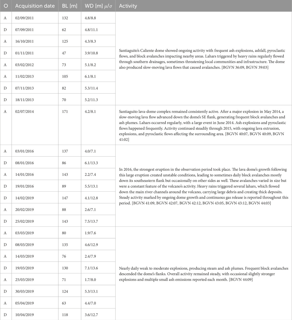
Table 1. Information on the TanDEM-X SAR images which were used for DEM generation. Provided are the acquisition date, the orbit (O, A = ascending orbit, D = descending orbit), the effective baseline (BL) in meters, the mean $\mu$ and standard deviation $\sigma$ of the difference between the individual DEMs and the WorldDEM (WD) in the reference areas in meters (see Section 2.5.3) as well as the activity within specific time intervals covered by the datasets. The activity was summarized from the bulletin reports published by the Global Volcanism Program (2025). The identifiers in the activity column provide information on the utilised Bulletin report(s) that can be consulted for more detailed information.

The DEM resolution is consistent in the North–South direction at 6.5 m for all scenes, but varies between 4 m and 6 m in the East–West direction. For analysis purposes and easy comparison, all datasets were resampled to a uniform 4 m resolution in the East–West direction. Table 1 provides further information on the data such as the effective baseline between the two TanDEM-X satellites, defined as half the length of the perpendicular baseline in the bistatic acquisition mode as well as an initial, brief overview over the activity at Santiaguito as reported in the bulletin reports of the Global Volcanism Program (2025). A detailed comparison of reported activity at Santiaguito and observations based on our data is presented in Section 4.1.

2.3 DEM generation

The DEM generation is based on InSAR, a method that uses the phase differences of two SAR images to derive information, in this case, on topographic heights. The interferogram is formed by multiplying one image with the complex conjugated of the other image and consists of amplitude and phase information. Generally, the phase information contains contributions from various factors such as surface deformation, topography and atmosphere, which have to be separated during the interferometric data processing pipeline (Hanssen, 2001). As mentioned in Section 2.1, TanDEM-X satellite products are especially well suited for volcanic regions as atmospheric effects and surface deformation are negligible (Kubanek et al., 2015a; Kubanek et al., 2015b; Kubanek et al., 2021).

Data processing and DEM generation for the present study were conducted using the open-source software DORIS (Delft Object-oriented Radar Interferometric Software; Kampes and Usai, 1999). This software was adapted by Kubanek et al. (2015b) in order to handle bistatic data. The individual processing steps are: (1) the coregistration of the two SAR images, (2) the formation of the interferogram, (3) the computation and subtraction of the reference phase and reference elevation, (4) the calculation of the coherence, (5) filtering, (6) phase unwrapping, (7) phase to height conversion and (8) geocoding and gridding. The details of the individual processing steps can be found in Kampes (1999). Unwrapping is not implemented in DORIS itself but uses the Statistical-Cost, Network-Flow Algorithm for Phase Unwrapping (SNAPHU; Chen and Zebker, 2001). The slant-to-height conversion and geocoding were performed using the Schwabisch algorithm implemented in DORIS (Schwäbisch, 1995).

Integrating a reference DEM during processing supports phase unwrapping and helps handle the underlying topographic effects and systematic distortions from the InSAR data (Hanssen, 2001; Gao et al., 2017). We initially used the WorldDEM (see Section 2.1) as a reference DEM for processing datasets from both, ascending and descending orbit. However, applying the WorldDEM to the ascending orbit datasets resulted in unwrapping errors. To address this issue, all ascending datasets were reprocessed using the DEM from 10/04/2019, as reference.

As a post-processing step, the ascending orbit DEMs, furthermore, underwent an additional vertical registration (Nuth and Kääb, 2011; Li et al., 2022) as we observed distinct discrepancies between the DEMs acquired from the different orbits. To correct for this as best as possible, individual correction ramps were applied to the ascending orbit datasets. Thereby, the WorldDEM was used as reference. The aim was to reduce the elevation difference between the individual scenes and the reference. Nevertheless, we were not able to completely remove the offset. The impact is discussed in Sections 2.5.2, 3 and 4.

2.4 Elevation and volume changes

2.4.1 Spatial subdivision of the area of interest

In this study, we investigate the elevation and volume changes both in the crater region as well as on the southern flank where, according to a manual preliminary assessment, activity concentrated during our observation period. To capture the spatio-temporal characteristics of these changes appropriately and compare the developments over time, we distinguished 10 different areas (see Figure 1). Area 1 encompasses the crater region which we furthermore subdivided into three different parts. This subdivision was based on an initial manual assessment of the spatio-temporal developments in the crater region and the resulting goal to properly account for opposing developments in different parts of the crater. Furthermore, we took the coherence in the crater region (see Figure 1) into consideration by defining Part 1 in a way that it encompasses the eastern half of the crater region without sufficient coherence for reliable analysis. The size of our Area 1 is 63,648 ${\mathrm{m}}^2$, which encompasses Part 1 of 28,626 ${\mathrm{m}}^2$, Part 2 of 12,428 ${\mathrm{m}}^2$ and Part 3 of 22,594 ${\mathrm{m}}^2$. The definition of the individual areas of Santiaguito’s southern flank is also based on an initial manual assessment of spatio-temporal elevation variations but also takes the outline of the flows included in the geologic map by Escobar Wolf et al. (2010) and the lava type map by Rhodes et al. (2018) into account. Escobar Wolf et al. (2010) present an updated version of the 1972 geological map, incorporating the evolution of the dome complex using aerial photographs, previous studies, unpublished field notes, and reports. Their map illustrates the geology of 34 distinct lava dome growth episodes and dome-collapse deposits. As a companion map to the map by Escobar Wolf et al. (2010), Rhodes et al. (2018) published the spatial distribution of lava types at Santiaguito based on aerial photographs and the results of a field campaign. Based on these two maps and our initial assessment, we define 9 areas on the southern flank with the following sizes: 142,324 ${\mathrm{m}}^2$ (Area 2), 67,392 ${\mathrm{m}}^2$ (Area 3), 290,628 ${\mathrm{m}}^2$ (Area 4), 89,544 ${\mathrm{m}}^2$ (Area 5), 534,742 ${\mathrm{m}}^2$ (Area 6), 575,328 ${\mathrm{m}}^2$ (Area 7), 562,848 ${\mathrm{m}}^2$ (Area 8), 721,968 ${\mathrm{m}}^2$ (Area 9) and 153,868 ${\mathrm{m}}^2$ (Area 10).

2.4.2 Elevation changes

By subtracting two of the generated DEMs pixel-wise, the local elevation changes in the time period between their respective dates of acquisition are derived. Applying the mask presented in Section 2.4.1 allows to evaluate the spatio-temporal patterns in elevation and volume change at Santiaguito volcano. For the flank, all available DEMs were used for analysis due to the presence of only a limited number of pixels with insufficient coherence (see Figure 2; Section 2.5.2). For the crater region, however, only DEMs acquired from the descending orbit were used as in the ascending orbit DEMs a considerable number of pixels with insufficient coherence were identified (see Figures 1, 2 as well as Section 2.5.2). The error in the observed elevation changes is determined and discussed in Section 2.5.

Figure 2

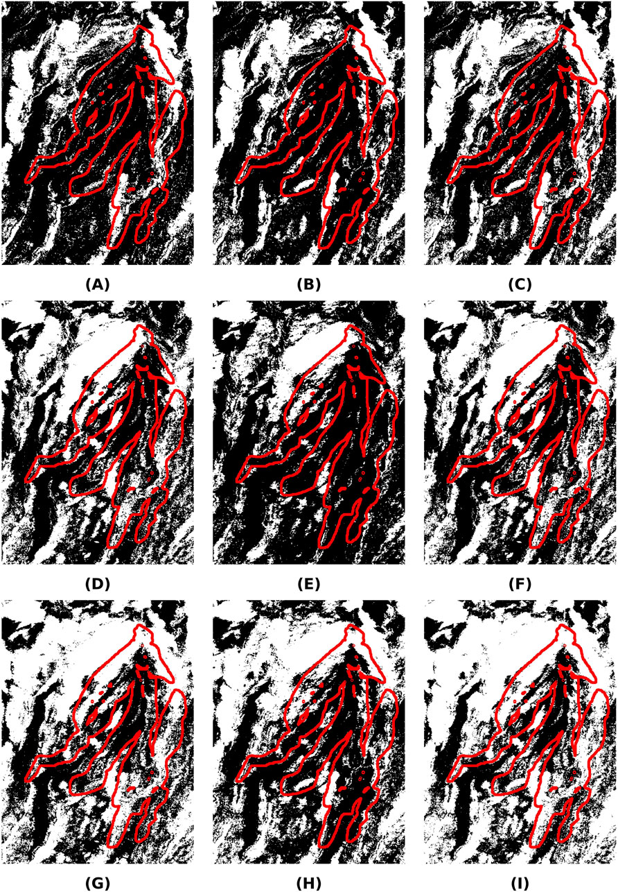
Figure 2. Coherence masks showing (A) Descending orbit DEMs (2011–2016), (B) Descending orbit DEMs (2019), (C) Descending orbit DEMs (2011–2019), (D) Ascending orbit DEMs (2011–2016), (E) Ascending orbit DEMs (2019), (F) Ascending orbit DEMs (2011–2019), (G) All DEMs (2011–2016), (H) All DEMs (2019) and (I) All DEMs (2011–2019). Coherence masks show in black all pixels that are equal or above the set coherence threshold of 0.4 for all considered DEMs. The red line marks the outline of the Areas 1–10 introduced in Figure 1.

2.4.3 Volume changes

Based on the local elevation changes determined for the individual areas shown in Figure 1, the corresponding volume changes $\mathrm{\Delta }{V}_i$ in ${\text{m}}^3$ can be computed using

$\mathrm{\Delta }{V}_i={\displaystyle \sum _{j=1}^n}A\cdot \mathrm{\Delta }{h}_j(1)$

where $n$ is the number of pixels in area $i$, $A$ represents the area of a single pixel in ${\text{m}}^2$, and $\mathrm{\Delta }{h}_j$ denotes the elevation change in pixel $j$ in m. Before calculating the volume changes, we remove pixels which, according to the coherence, show less reliable information and interpolate their values linearly from the remaining pixels.

From the volume changes in a specific time interval, the average volume output rate $\mathrm{\Delta }{V}_{i,avg}$ in ${\text{m}}^3$/s can be calculated as

$\mathrm{\Delta }{V}_{i,avg}=\mathrm{\Delta }{V}_i/\mathrm{\Delta }t(2)$

where $\mathrm{\Delta }$t is the time in seconds between the acquisition of the two DEMs used to derive $\mathrm{\Delta }{V}_i$. A negative average volume output rate corresponds to a volume decrease.

2.5 Errors in the determined elevation changes

2.5.1 Relative elevation errors

Assessing the magnitude of the errors contained in the determined elevation and volume changes is essential to correctly interpret the results. In this study, we follow an approach introduced by Kubanek et al. (2017). We define 6 reference areas (A- F, see Figure 3) that we assume are stable in elevation, i.e., they are not affected by volcanic or other natural changes over the time of the study. As a basis for defining these areas, we first consulted our data to rule out areas affected by significant elevation changes either due to volcanic activity or secondary transport processes. Furthermore, satellite images helped constrain landmarks unsuitable to be included in the reference areas such as large river beds. The elevation change determined from two “perfect” DEMs would, therefore, yield 0 m in these reference areas. As a consequence, the actually occurring elevation changes in the reference areas act as a way to quantify the error. This approach does not indicate the absolute errors of the individual DEMs but only assesses the relative error in the difference between two DEMs. For the investigations of elevation and volume changes as conducted in this study this approach of error determination is well suited as only the elevation differences are being analyzed and not single DEMs. Because much of the area surrounding Santiaguito is vegetated defining suitable reference areas proved challenging. We placed reference areas of various sizes in mostly vegetation-free regions, though some include vegetation. As the initial investigation of the DEMs revealed no changes on other parts of Santiaguito apart from the southern flank and crater, two reference areas are also located on the northern and western flank respectively.

Figure 3

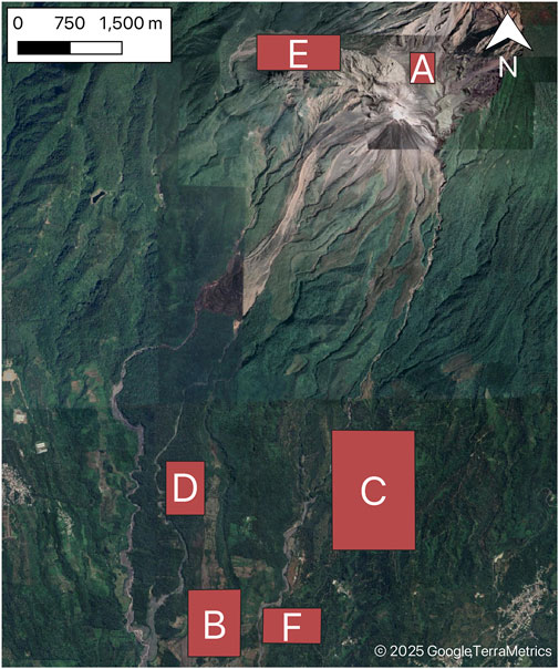
Figure 3. Location and size of the 6 reference areas A- F defined for determining the errors contained in the determined elevation changes. Background image: ©2025, Google TerraMetrics.

We determined the relative error for each pair of DEMs used to derive elevation or volume change information in this paper. Each pixel within each reference area was assessed and from all pixels, the mean and standard deviation were then calculated over all reference areas. Figure 4 shows the results for pairs of consecutive DEMs and DEM combinations with the first DEM of the observation period as reference. The mean deviation varies between −3.8 m and 4.6 m. The standard deviation ranges from 2.5 m to 7.3 m. Following Kubanek et al. (2017), we integrate the standard deviation as magnitude of errors in the elevation changes. These errors represent random errors resulting, e.g., from noise. We assume that they apply uniformly across the entire scene. Additional error sources, such as systematic topographic effects caused, for example, by geometrical decorrelation in steep terrain, are not considered. The error of the calculated volume change in area $i$, $\mathrm{\Delta }{V}_{i,E}$ in ${\text{m}}^3$, can consequently be calculated as follows:

$\mathrm{\Delta }{V}_{i,E}=n\cdot A\cdot E$

where $n$ is the number of pixels in $i$, $A$ represents the area of a single pixel in ${\text{m}}^2$, and $E$ denotes the error in the elevation change in m.

Figure 4

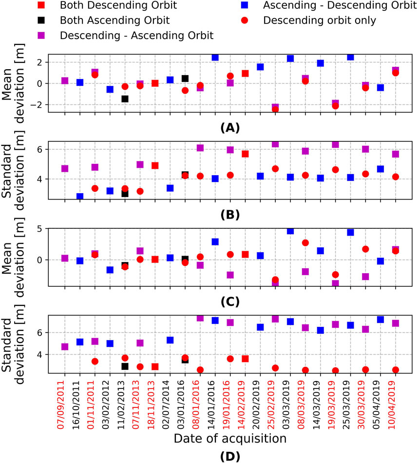
Figure 4. The figure shows the magnitude of errors contained in the differences between the DEMs used in this study to assess elevation and volume changes. It includes both differences between consecutive DEMs (C,D) and differences relative to the first DEM (A,B). In (C,D), square markers correspond to errors calculated relative to the previous DEM in time, regardless of orbit, whereas round markers refer to errors relative to the previous descending orbit DEM. In (A,B), square markers are referenced to 02/09/2011, while round markers refer to 07/09/2011. The red dates of acquisition in the axis label mark the DEMs acquired from the descending orbit. The color-coding of the markers refers to the combination of orbits.

2.5.2 DEM quality based on coherence information

Section 3 highlights notable discrepancies between the results derived from ascending and descending orbit DEMs, particularly in the western part of the southern flank (Areas 4 and 5). They likely stem from offsets that are still contained in the DEMs of the ascending orbit despite the applied vertical correction efforts (see Figure 5). We attribute these offsets primarily to topographic effects such as geometrical decorrelation.

Figure 5

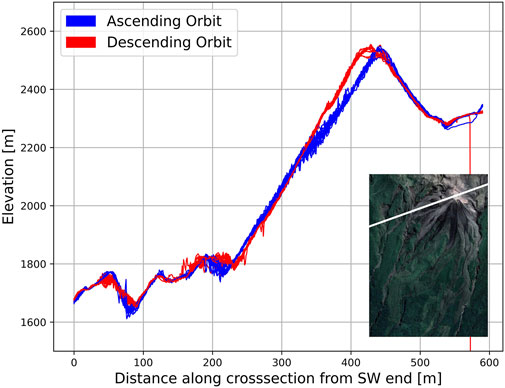
Figure 5. Elevation along a crosssection extracted from all DEMs. The color-coding distinguishes between the orbits of the DEMs. The location of the crosssection is illustrated as a white line in the image at the bottom right corner. Image: ©2025, Google satellite, Airbus, CNES/Airbus, Landsat/Copernicus, Maxar Technologies.

Coherence masks, derived separately for ascending and descending orbit data, provide information on spatial coherence variations. To generate these masks, we consider the pixel-wise coherence values of all relevant scenes. A threshold of 0.4 is used to classify coherence as “sufficient” or “insufficient,” based on prior experience. Pixels are marked as having insufficient coherence if at least one scene shows a value below this threshold. Figure 2 displays the resulting coherence masks for ascending and descending orbit DEMs, as well as a combined mask for all DEMs. Pixels with insufficient coherence (i.e., below the threshold in any DEM) are shown in white.

Analysis of these masks reveals that ascending orbit scenes generally exhibit slightly fewer pixels with sufficient coherence than descending orbit scenes, particularly in the west and northeast. This might be an indication that for the above mentioned Areas 4 and 5 in the western part of the flank the descending orbit data might provide more reliable results than the DEMs of the ascending orbit. This does less affect the visual interpretation of elevation changes but rather the calculated volume changes (see Section 3.2.2). Nevertheless, overall, we conclude that the southern flank remains a reliable area for analysis using DEMs from both orbits. During volume change calculation, we identify pixels of low coherence, and use the surrounding pixels of sufficient coherence for their interpolation. Thereby, we only access the low coherence pixels of either of the two DEMs included in the volume change determination and not all pixels with insufficient coherence in the aggregated coherence masks shown in Figure 2 that consider all DEMs. As a result, the coherence masks for pairs of DEMs used for volume change determination, generally, contain significantly more pixels with sufficient coherence. When discussing our results in Section 4, we consider the spatial coherence distribution in our interpretation to avoid misinterpretation of unreliable data.

Discrepancies in coherence between the orbits are particularly pronounced in the crater region. While descending orbit scenes display sufficient coherence in the western half of the crater, ascending scenes lack the quality needed for reliable analysis. We assume this to be related to the anomalous behavior in ascending orbit data near the crater as visible in Figure 5. As a result, the crater region is analyzed using only descending orbit DEMs. However, due to insufficient coherence in the eastern half, our assessment is limited to the western half of the crater.

Figure 2 distinguishes between DEMs from the periods 2011–2016, 2019, and 2011–2019. A comparison of the coherence masks from different periods reveals no significant change in coherence patterns. Therefore, the reliability of the DEMs can be assumed to remain consistent throughout the observation period.

2.5.3 DEM quality with respect to the WorldDEM

Even though this study is purely based on the relative elevation changes of the produced DEMs that were generated under equal circumstances, we applied the reference areas defined in Section 2.5.1 for comparison of the individual DEMs with the WorldDEM (see Section 2.1). This comparison is not intended as a full accuracy validation but rather as an independent indication of DEM quality and consistency. Since no significant elevation changes due to volcanic activity are expected in the reference areas, differences relative to the WorldDEM provide a reasonable benchmark for assessing the internal consistency of our DEMs.

Table 1 reports the mean and standard deviation of the differences of all pixels in the six reference areas. The DEMs exhibit a positive bias relative to the WorldDEM (mean difference >0 m for all DEMs), indicating a slight upward offset. The standard deviations range from 7.0 m to 13.7 m. Compared to the mean and standard deviation values presented in Section 2.5.1 (see Figure 4), the maximum standard deviations of the present comparison are slightly higher. We can also observe a dependence on the acquisition orbit with the standard deviation being smaller for ascending orbit DEMs.

Comparing all mean and standard deviations in Table 1 shows that their variations are sufficiently small to support the claim of similar quality among all DEMs. This is the most essential information for our study, as we focus on substantial elevation changes that are significantly larger than the standard deviations shown in Figure 4. Thus, while the detected offsets would need to be considered if combining these DEMs with external elevation datasets, for our relative-change analysis they do not significantly affect the reliability of the results.

3 Results

3.1 Developments in the crater region

3.1.1 Elevation changes

As discussed in Section 2.4.2, 2.5.2, the elevation changes in the crater region were investigated only based on the descending orbit DEMs (see Table 1) due to insufficient coherence of the DEMs acquired from the ascending orbit. For the same reason, the descending orbit DEMs were only evaluated in the western half of the crater region, which was further distinguished in the northern Part 2 and southern Part 3 (see Section 2.4.1). Figure 6 shows the changes in elevation in the crater region in selected time intervals. Figure 7 respectively illustrates the spatio-temporal developments with respect to the first DEM of the descending orbit acquired on 07/09/2011.

Figure 6

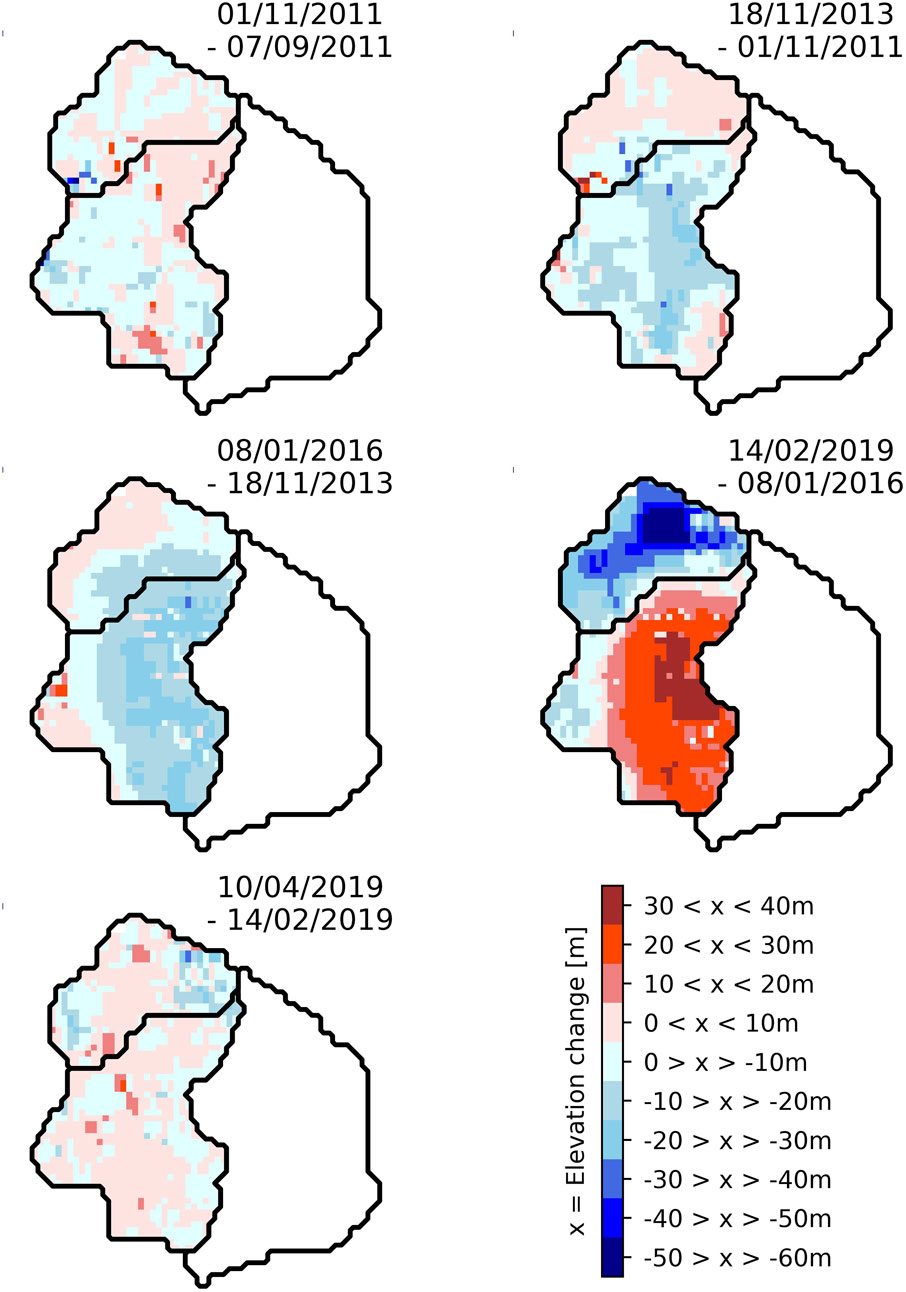
Figure 6. Elevation changes in the western half of the crater region (Area 1) determined from the two DEMs acquired on the provided dates. Values were discretized for better visibility.

Figure 7

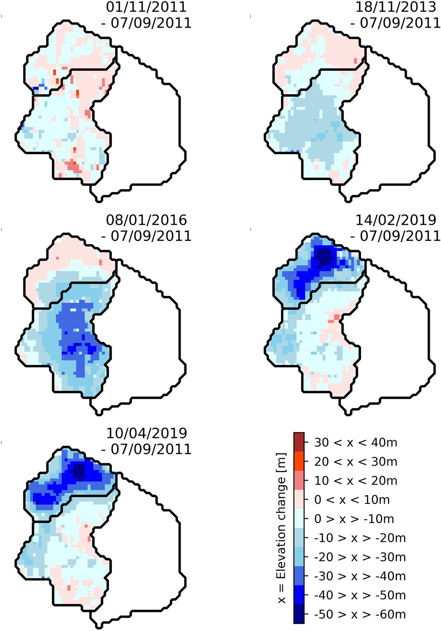
Figure 7. Elevation changes in the western half of the crater region (Area 1) between the DEMs acquired on the provided dates and the first DEM of the descending orbit acquired on 07/09/2011. Values were discretized for better visibility.

Between 2011 and 2016, elevation reduced around 40 m towards the center of the crater region (Part 3). Between 2016 and 2019, we observed an increase in elevation, again, especially towards the middle of the crater (Part 3), almost leveling the previous reduction in elevation. In the same time period, the north-western crater rim (Part 2) decreased by almost 60 m. In the first 4 months of 2019, which also mark the end of the observation period, a slight increase in elevation of the crater region can be observed. However, comparably small developments of up to $\pm$10 m, which are, therefore, close to the determined uncertainties in the elevation differences (see Section 2.5), need to be interpreted with caution.

3.1.2 Volume changes

Based on Equation 1, we determined the spatio-temporal volume changes. Figure 8 illustrates the volume changes in Part 2, 3 and the entire western half of the crater region between consecutive DEMs. Figure 9 illustrates the development with respect to the first DEM acquired from the descending orbit.

Figure 8

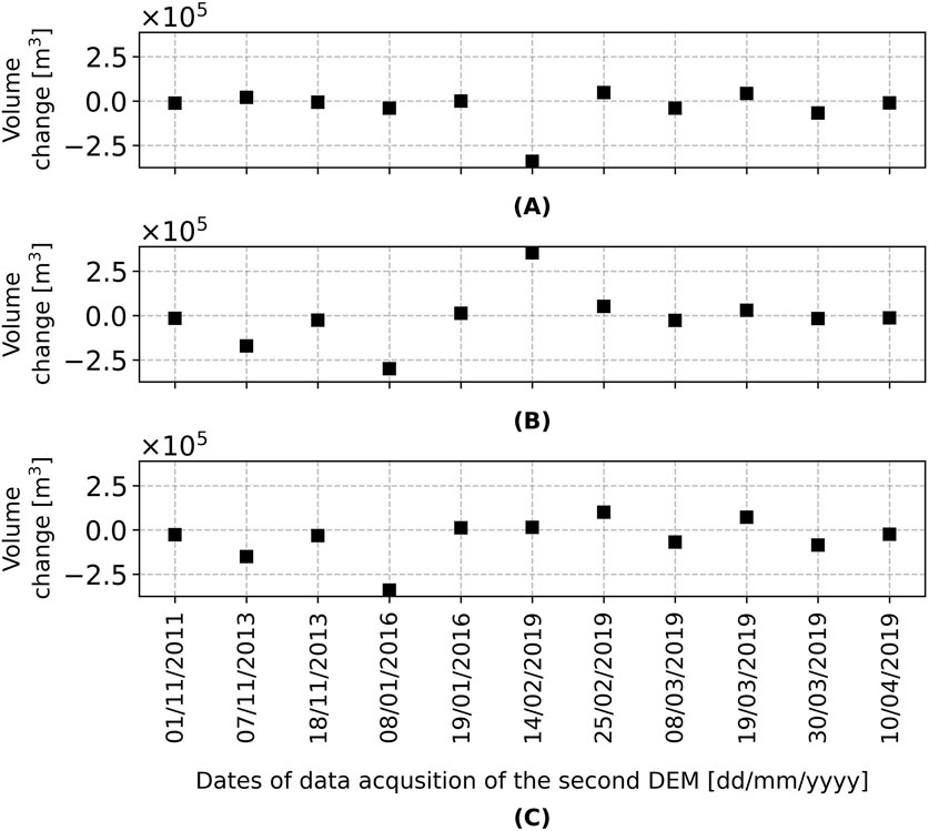
Figure 8. Volume changes in the crater region between two consecutive DEMs of the descending orbit in (A) Part 2, (B) Part 3 and (C) the entire western half of the crater region. The markers are assigned to the later date of acquisition involved in the assessment.

Figure 9

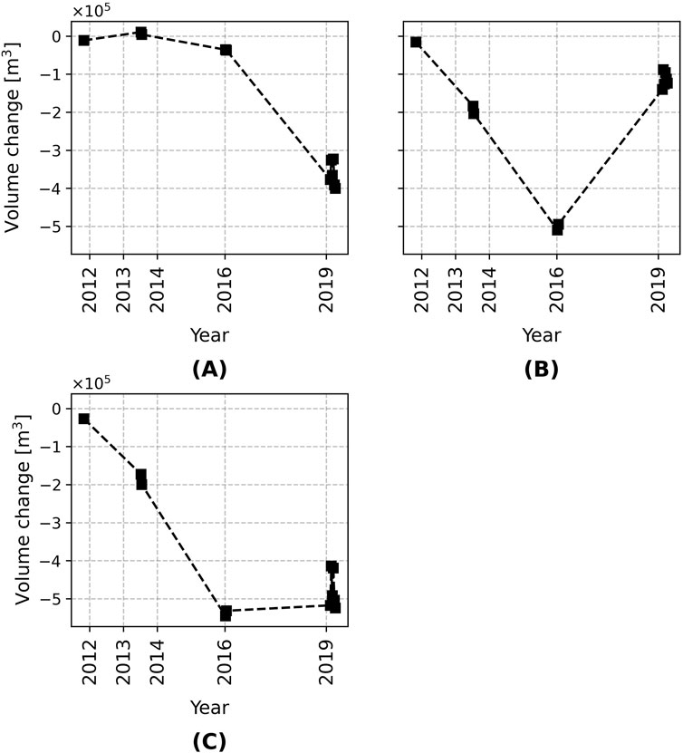
Figure 9. Volume changes with respect to the first DEM of the descending orbit acquired on 07/09/2011 in (A) Part 2, (B) Part 3 and (C) the entire western half of the crater region.

The volume change patterns in the crater align with the elevation changes described in Section 3.1.1. In Part 2, no significant change occurs until 2016, when the north-western crater rim drops, reducing the volume by (377 $\pm$ 2)$\cdot 10^3$ ${\mathrm{m}}^3$. Part 3 shows a volume decrease until early 2016, totaling (495 $\pm$ 4)$\cdot$ ${10}^3$ ${\mathrm{m}}^3$. Volume increase begins in 2016, and by 2019, the volume difference compared to the start of observations comes out at only (−140 $\pm$ 4)$\cdot 10^3$ ${\mathrm{m}}^3$. The magnitude of these opposing changes in Part 2 and 3 nearly balances out, resulting in no significant overall volume increase or decrease between 2016 and the end of the observation period. However, the developments in Part 3 mark the volcanologically more relevant development.

The average volume output rate in the crater region calculated from consecutive DEMs using Equation 2 is shown in Figure 10, distinguishing between the entire western crater region and individual Parts 2 and 3. The largest change, a decrease of 3.93 $\pm$ 0.04 ${\text{m}}^3$/s, occurred mainly in Part 3 between 18/11/2013 and 08/01/2016. Between 19/01/2016 and 14/02/2019, the overall average output rate is nearly zero, but this results from opposite developments in Parts 2 and 3. With an average volume output rate of 4.1 ${\mathrm{m}}^3$/s in Part 3, however, the most significant changes in the crater region occurred during this time interval.

Figure 10

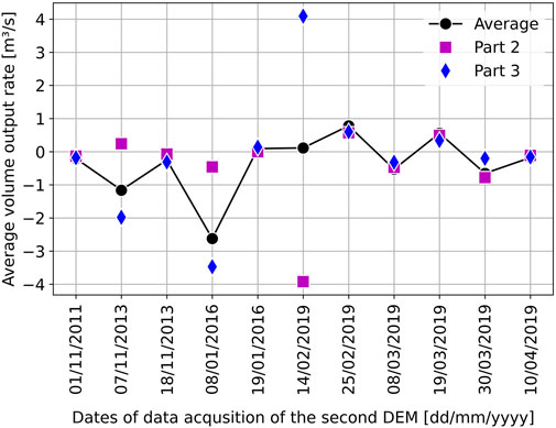
Figure 10. Average volume output rate as calculated from the crater region. Values were determined between two consecutive DEMs of the descending orbit. The markers are assigned to the later date of acquisition involved in the assessment.

Figure 11 shows the average volume output rate relative to the first DEM from 07/09/2011. Over the entire observation period, the average volume output rate was (−219 $\pm$ 2) $\cdot 10^{-5}$ ${\mathrm{m}}^3$/s. The output rates are predominantly negative, reflecting the substantial volume loss in the western half of the crater region, first in Part 3 and then in Part 2. However, the magnitudes of these crater-derived output rates are small and do not significantly influence Santiaguito’s overall volume output rate (compare Section 3.2.2).

Figure 11

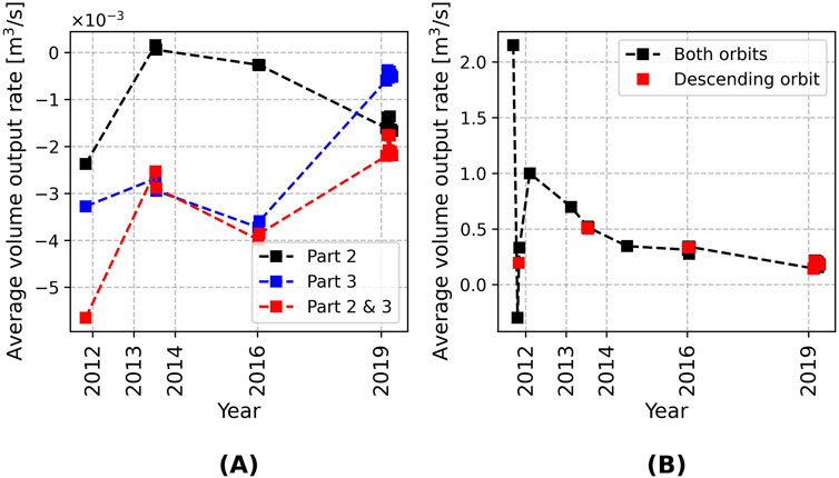
Figure 11. Average volume output rate (A) in the crater region and (B) on the southern flank. The output was determined with respect to the first DEM of the considered orbit, i.e. 07/09/2011 for the crater region and the descending orbit assessment for the southern flank and otherwise 02/09/2011 for the southern flank in general. For the southern flank, Areas 2, 4 and 5 are not included (see Section 4.1).

3.2 Developments on Santiaguito’s southern flank

3.2.1 Elevation changes

Figure 12 shows the elevation changes on the flank relative to the DEM acquired on the date of the preceding image. The changes on the first image were determined with respect to the first DEM of the observation period. Figure 13 illustrates the spatio-temporal elevation changes between the provided date of acquisition and the first DEM of the observation period.

Figure 12

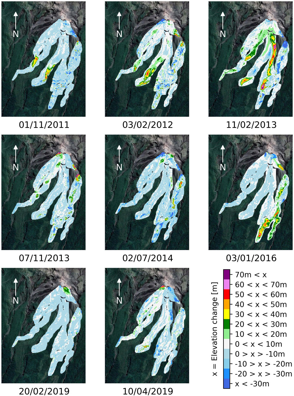
Figure 12. Elevation changes on the southern flank (Areas 2–10). Values were discretized for better visibility. The elevation changes were determined between the DEM acquired on the provided date and the DEM acquired on the date of the preceding image. The first image was determined with respect to the first DEM of the observation period. Background images ©2025, Airbus, CNES/Airbus, Landsat/Copernicus, Maxar Technologies.

Figure 13

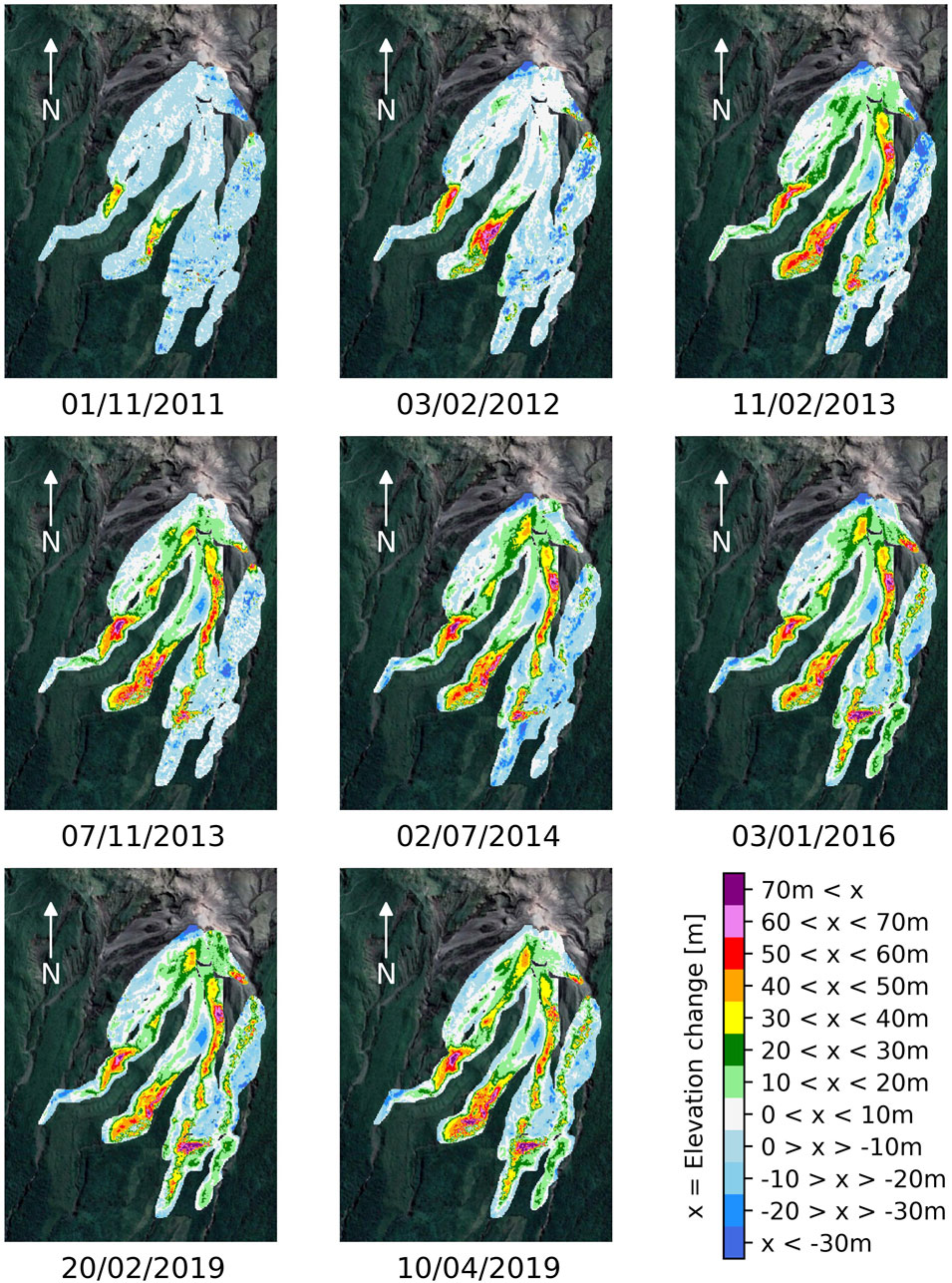
Figure 13. Elevation changes on the southern flank (Areas 2–10). Values were discretized for better visibility. Displayed is the elevation change at selected points in time with respect to the first DEM of the observation period. Background images ©2025, Airbus, CNES/Airbus, Landsat/Copernicus, Maxar Technologies.

The majority of the displayed elevation changes is colored either white or light blue, indicating comparably small magnitudes of up to $\pm 10$m. Given the uncertainties in the elevation changes discussed in Section 2.5, we interpret these changes with caution. We will focus on the prominent changes that are significantly larger than the determined errors. In the first 2 months of the observation period, an accumulation of material can be observed in Areas 6 and 7. This accumulation increased until the beginning of 2012. More extensive elevation changes occurred between February 2012 and February 2013. In Area 8, material accumulated several hundreds of meters down the slope. We observed also material accumulation in the upper half of Area 6. Furthermore, the accumulation of material in Area 7 extended in size further down the slope. Through 2013 until July 2014 only little change is visible. Between July 2014 and the beginning of 2016 changes occurred mainly in Areas 9 and 10 in the eastern part of the flank. From 2016 onward, hardly any material accumulated on the flank with most changes occurring close to the crater in Area 2.

3.2.2 Volume changes

Similarly to the crater region in Section 3.1.2, we determined the volume changes on Santiaguito’s southern flank for each of the 9 areas individually. We based our analysis on volume changes relative to the first DEM from 02/09/2011, as this makes the observed developments easier to interpret than changes between consecutive DEMs. Figure 14 illustrates the volume changes in the individual areas with respect to the first DEM of the observation period.

Figure 14

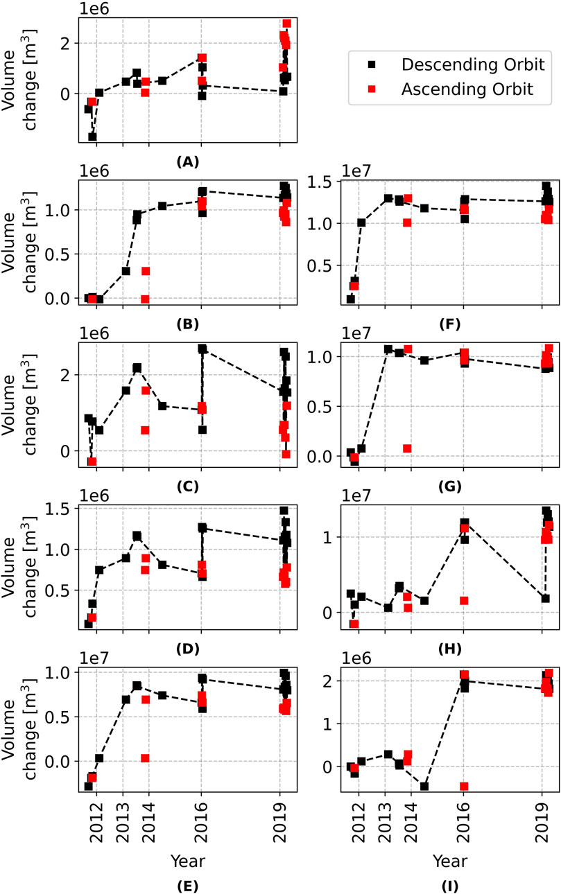
Figure 14. Volume changes on Santiaguito’s flank for (A) Area 2, (B) Area 3, (C) Area 4, (D) Area 5, (E) Area 6, (F) Area 7, (G) Area 8, (H) Area 9 and (I) Area 10. Values were determined with respect to the first DEM of the observation period. The color indicates the orbit of the non-reference DEM. For interpretation of results diverging due to the analysis of DEMs acquired from different orbits, refer to Section 2.5.2.

The spatio-temporal pattern of volume change follows the pattern of the elevation changes described in Section 3.2.1. The largest changes occurred in Areas 6, 7, 8 and 9, as these are also the largest areas. We observe that the determined volume changes are affected by the combination of DEMs, i.e., the orbits from which they were acquired (see Section 2.5.2).

Figure 11 shows the average volume output rate with respect to the first DEM of the observation period determined using Equation 2. The average volume output rate decreases in the second half of the observation period, matching the pattern of reduced lava emplacement on the flank. The strong fluctuations of the average volume output rate determined from DEMs of both orbits between September 2011 and the beginning of 2012 most likely result from the temporally closely spaced DEMs that were acquired from different orbits and contain the discrepancies discussed in Section 2.5.2. Therefore, following the descending orbit-only average output provides a reliable trend assessment of the average volume output rate. Based on this, we determined a rate of 0.2 $\pm 0.0004$ ${\mathrm{m}}^3$/s over the entire observation period. When excluding Areas 2, 4 and 5 due to volume changes potentially caused by secondary transport processes and reduced reliability as indicated by insufficient coherence (see Sections 2.5.2, 4), the average volume output rate is 0.18 $\pm 0.0004$ ${\mathrm{m}}^3$/s. Between 2011 and 2016, the rate is calculated as 0.4 $\pm 0.001$ ${\mathrm{m}}^3$/s or 0.3 $\pm 0.0008$ ${\mathrm{m}}^3$/s respectively.

4 Discussion

4.1 Comparison with volcanic activity reported in literature

This study uses TanDEM-X-derived DEMs to quantify elevation and volume changes at Santiaguito between 2011 and 2019. Although the datasets were acquired at irregular intervals, the observed cumulative changes provide meaningful insights into the volcano’s morphological evolution during this period. In the following, we compare our observations with reports from the Global Volcanism Program (2025) and several published studies on Santiaguito’s development. Overall, these reports describe similar activity at Santiaguito during our period of observation compared to previous decades. They also highlight the variety of activity at the volcano that can lead to changes in elevation including primary processes, such as lava flows and secondary transport processes like lahars. The strongest eruption during our observation period occurred in 2016 which is described in detail by the Global Volcanism Program (2025) and Lamb et al. (2019). While the irregular temporal coverage of the data limits our ability to attribute changes to specific eruptive events, integrating diverse sources supports us in distinguishing between surface changes related to lava emplacement and those driven by other processes. Furthermore, these external sources allow an assessment of the validity of our results.

In the western crater region, we observe two contrasting developments during the periods 2011 to 2016 and 2016 to 2019 which are visible in Figures 6–9. Between 2011 and 2016, Part 3, which includes parts of the crater center, experienced significant subsidence and associated volume loss. This trend intensified between 2013 and 2016 (see Figure 9). The volume decrease during this period may be attributed to dome collapse processes, as discussed by Calder et al. (2002) and Carr et al. (2022). The reports by the Global Volcanism Program (2025) describe dome collapse events in the summers of 2012 and 2013. Lamb et al. (2019), based on field observations and geophysical monitoring from 2014 to 2017, also document a dome collapse on 9 May 2014, primarily affecting the eastern part of the crater, which, however, is outside our analysis area. Massaro et al. (2022) describe episodic activation of the shallow and intermediate magmatic systems between 2011 and 2015, which they attribute to likely involving pressurization and depressurization cycles, a process associated with dome instability (Voight and Elsworth, 2000). The degassing observations in the summers of 2013 and 2014, as reported by the Global Volcanism Program (2025), may support their claim. In 2015–2016 Santiaguito experienced increased eruptive intensity, which Wallace et al. (2020) link to the influx of hotter, volatile-rich magma. Comparing the DEMs from 2016 to 2019, we observe significant volume loss in the northwestern crater region (Part 2), potentially consistent with Lamb et al. (2019) and the Global Volcanism Program (2025), who report significant morphological changes including rim excavation in the crater region following Santiaguito’s strong 2016 eruption. Meanwhile, in Part 3, which previously experienced volume loss, we now observe renewed material accumulation. This aligns with descriptions by Lamb et al. (2019) and the Global Volcanism Program (2025), who report dome growth and increasing material accumulation in the crater during this period. Overall, the agreement between our DEM-derived results and published observations supports the reliability of our data and interpretation for the crater region, even in the absence of event-level temporal resolution.

On the southern flank, we observe the emplacement of several lava flows especially between 2011 and 2016, while there were hardly any changes between 2016 and 2019 (see Figures 12–14). From the beginning of the observation period until February 2012, we observe localized mass accumulation at the southern ends of Areas 6 and 7. These changes are spatially limited and occur well outside the crater region. The lava type map in Rhodes et al. (2018) as well as the study by Ebmeier et al. (2012) mention lava flow emplacement in mid-2011 in these areas. Given the distal location of the observed accumulation, our observed volume changes are more likely associated with secondary transport processes of previous deposits than direct eruptive deposition. This is reasonable as reports from the Global Volcanism Program (2025) document instances of material displacement by lahars, pyroclastic flows and avalanches from lava flows during this time period. Between 2012 and 2013, Area 6 experienced volume increase again, however, on the upper part of the slope. Therefore, these changes can be interpreted as new material emplacement. The most significant change of this period occurred in Area 8 where mass accumulation occurred over its entire length, which we attribute to the same lava flow event resulting in the accumulation in the north of Area 6. This interpretation is generally supported by the Global Volcanism Program (2025) that reports in the week of 5–11 December 2012 the emplacement of a new 700 m long lava flow in this time period on the southern flank. In Area 7, the strongest changes occur at the southern end of the area. As they are far from the crater and further up the slope elevation decrease is visible, we interpret these changes as due to secondary mass transport as well. Further material accumulation at the northern end of the area, however, is new lava being emplaced just as in Areas 6 and 8.

Between 2013 and July 2014, we did not observe much activity on the flank, apart from some changes in Area 9. Investigations of the DEMs involved in the assessment show slightly lower coherence in Area 9 than later DEM pairs, so the patchy-pattern changes might not reflect in full actual elevation changes but might be partially due to artifacts. Between July 2014 and January 2016, at the southern end of Area 2 as well as over the entire length of Area 9 and 10, we observe material accumulation. Thereby, most material was added on the southern end of Area 9 and in Area 10. The map by Rhodes et al. (2018) provides the onset of the lava flow in Areas 9 and 10 for May 2014. When Lamb et al. (2019) discuss the collapse of the lava dome in May 2014, the authors identify the resulting changes in the eastern crater rim as the origin of the lava flows in Areas 9 and 10. This is supported also by the reports by the Global Volcanism Program (2025) that describe the descend of lava flows in the east following the 9 May 2014 eruption. This shows that this mass accumulation is due to lava flow activity. Overall, the lack of changes reported by Rhodes et al. (2018) and Lamb et al. (2019) previous to mid-2014 in Areas 9 and 10 support the claim above that the volume changes that we previously observed in this area in our data are a result of artifacts. Later observations of the development of a lava flow in these areas between 2014 and 2016 are, however, in accordance with literature.

Between 2016 and 2019, hardly any change can be observed on the flank apart from accumulation of material in Area 2 close to the crater region. The long interval between DEM acquisitions may have led to the loss of detailed information on developments such as those associated with the 2016 Santiaguito eruption. Erosion in-between acquisition intervals, for example, can cause an underestimation of derived volume change patterns (Ebmeier et al., 2012).

Figures 12–14 show that, in contrast to the crater region, there is no prolonged, systematical volume decrease visible on the southern flank. The maps show that most decreases range close to the determined elevation errors (see Figure 4) and therefore need to be interpreted with caution. We account the elevation decrease visible in the NW corner of Area 4 to be an artifact due to the in Figure 5 displaced discrepancy between both orbits’ DEMs in this area. Similarly, as also outlined above, we interpret elevation reductions in Area 9 with caution. Ebmeier et al. (2012) who investigated also subsidence at Santiaguito between 2000 and 2009 found in their study a subsidence rate of up to 6 cm/year, which is too small to be recognized in our study. Therefore, we attribute any reliable volume decrease to secondary mass transport.

Overall, the strong agreement between our results and the volcanic activity discussed in literature and reports for both the crater region as well as the flank strengthens the trust in our study. However, both the literature and our own data show that activity is primarily concentrated in the crater region and on the S and SE flank. We could not identify sources clearly discussing mass movements in Areas 4 and 5. This may indicate that any changes observed may be due to secondary mass movement. However, especially Area 4 but also Area 5 overall across all DEM differences have the lowest coherence indicating a reduced reliability. Area 2 also shows a reduced coherence in the DEM differences, even though the elevation change patterns in this area seem reasonable. Nevertheless, this shows that caution should be exercised when interpreting these areas. The ambiguous development of the volume changes in Figure 14 in these areas may on the one hand be attributed to the lack of sufficient coherence but, especially for Areas 4 and 5, could also support the interpretation as changes due to secondary transport processes.

4.2 Average volume output rates

Harris et al. (2003) reported a discharged volume of (1.1–1.3)$\cdot 10^{10}$ ${\mathrm{m}}^3$ between 1922 and 2000, and Ebmeier et al. (2012) determined a volume increase of (1.2 $\pm$ 0.1)$\cdot 10^8$ ${\mathrm{m}}^3$ from 2000 to 2009. Massaro et al. (2022), who investigated the development of the discharge rates of Santiaguito from 1922 to 2021 based on published literature and satellite thermal data, found a volume increase of (202 $\pm$ 101)$\cdot 10^6$ ${\mathrm{m}}^3$ between 2000 and 2021. Over our entire observation period, we observed material accumulation of (44 $\pm$ 0.1)$\cdot 10^6$ ${\mathrm{m}}^3$ when excluding Areas 2, 4 and 5 and (46 $\pm$ 0.1)$\cdot 10^6$ ${\mathrm{m}}^3$ when including all areas. Compared to the published literature our results seem reasonable. The exclusion of Areas 2, 4, and 5 is motivated in Section 4.1, which shows that these areas are particularly affected by low coherence and, in the case of Areas 4 and 5, may reflect secondary mass movements rather than primary volcanic deposition. However, due to their limited spatial extent, omitting these areas has only a minor impact on the overall volume estimates.

We determined the average volume output rate over the entire observation period to be 0.18 $\pm$ 0.0004 ${\mathrm{m}}^3$/s without considering Areas 2, 4 and 5 and 0.2 $\pm$ 0.0004 ${\mathrm{m}}^3$/s including all areas. These values match the average output rate during the low discharge sequence of Santiaguito’s cyclic pattern determined by Harris et al. (2003). However, we observed changes of the average volume output rate over the observation period. With 0.5 $\pm$ 0.001 ${\mathrm{m}}^3$/s (without Areas 2, 4 and 5) and 0.6 $\pm$ 0.002 ${\mathrm{m}}^3$/s (all areas), the rate between 2011 and November 2013 corresponds with a phase of high discharge. Ebmeier et al. (2012) state that 2000 to 2005 as well as 2011 to early 2012 were intervals of high discharge. Hornby et al. (2019) observed that discharge declined through 2014 and then ceasing in December. A similar temporal development has been found by Massaro et al. (2022). Our results showing first high discharge at the beginning of our observation period followed by a drop in the average volume output rate aligns with these previous observations. The total length of the high discharge period then aligns also with the typical length of such a period as given in Harris et al. (2003). The drop then might indicate the start of a period of low discharge. However, the significant discharge in Part 3 in the crater region between 2016 and 2019 (see Figure 10) due to the strong dome growth should not be disregarded.

Harris et al. (2003) observed that the eruption rate for each cycle decreased over time and cycle duration increased. Furthermore, the authors describe a reduction of the maximum discharge rates during each cycle after 1958. Our data seem to be in agreement with the discharge rates published by Harris et al. (2003) and Ebmeier et al. (2012). The average volume output rate between 2011 and 2013 is at the lower end of or slightly below the interval of rates associated with the phase of high discharge, potentially supporting the assumed long-term decrease of discharge rates.

4.3 Conclusion

This study used TanDEM-X derived DEMs to quantify elevation and volume changes at Santiaguito volcano between 2011 and 2019. Our analysis demonstrates that bistatic InSAR is a valuable tool for monitoring active volcanoes and capturing their morphological evolution over time.

Over the entire observation period, we detected a cumulative volume increase of $(44\pm 0.1)\cdot 10^6$ ${\mathrm{m}}^3$, corresponding to an average volume output rate of $0.18\pm 0.0004$ ${\mathrm{m}}^3$/s (excluding low coherence areas). We interpret these values to be consistent with previously published long term discharge and corresponding discharge rates. Our results indicate a phase of elevated volcanic activity between 2011 and 2013, with an average volume output rate of $0.5\pm 0.001$ ${\mathrm{m}}^3$/s (without low coherence areas). After 2013, a decline in discharge suggests a transition into a lower activity phase. This temporal pattern aligns with previous studies reporting cyclicity at Santiaguito. In the western crater region, we observed subsidence between 2011 and 2016. Following a major eruptive event in 2016 and a possible shift in magmatic activity (Lamb et al., 2019; Wallace et al., 2020), we detected substantial renewed material accumulation and dome growth, especially near the crater center. On the southern flank, lava emplacement was largely observed in the period from 2011 to 2016, with limited activity thereafter. Our interpretation of these flank changes, distinguishing between primary lava emplacement and secondary mass transport as best as possible given the limitations of the study, is supported by coherence analyses and independent literature.

Despite limitations such as irregular DEM acquisition intervals and lower coherence in some areas, the strong agreement between our results and external data sources confirms the validity of our approach and our results. Overall, this study contributes to a more detailed understanding of Santiaguito’s recent evolution, and demonstrates the potential of TanDEM-X data for long term volcano monitoring.

Data availability statement

The data analyzed in this study is subject to the following licenses/restrictions: We accessed the TanDEM-X data, provided by the German Aerospace Center (DLR), under proposals NTI_INSA0405 and OTHER0653. Our work is subject to DLR’s data access and usage guidelines. Requests to access these datasets should be directed to https://tandemx-science.dlr.de/.

Author contributions

A-KE: Formal Analysis, Writing – review and editing, Writing – original draft. JKu: Methodology, Data curation, Supervision, Writing – review and editing. EG: Project administration, Writing – review and editing, Supervision, Conceptualization. AD: Writing – review and editing, Supervision. MW: Project administration, Methodology, Conceptualization, Supervision, Writing – review and editing. JKo: Resources, Writing – review and editing. AR: Project administration, Supervision, Conceptualization, Writing – review and editing.

Funding

The author(s) declare that financial support was received for the research and/or publication of this article. Open access funding provided by the Open Access Publishing Fund of RWTH Aachen University.

Acknowledgments

We would like to thank Hansjörg Kutterer and Bettina Kamm (both from the Karlsruhe Institute of Technology) for their support and supervision. We thank the reviewers for their constructive feedback, which helped us to improve this manuscript. This study was performed as part of the Helmholtz School for Data Science in Life, Earth and Energy (HDS-LEE).

Conflict of interest

The authors declare that the research was conducted in the absence of any conflict of interest.

Generative AI statement

The author(s) declare that no Generative AI was used in the creation of this manuscript.

Any alternative text (alt text) provided alongside figures in this article has been generated by Frontiers with the support of artificial intelligence and reasonable efforts have been made to ensure accuracy, including review by the authors wherever possible. If you identify any issues, please contact us.

Publisher’s note

All claims expressed in this article are solely those of the authors and do not necessarily represent those of their affiliated organizations, or those of the publisher, the editors and the reviewers. Any product that may be evaluated in this article, or claim that may be made by its manufacturer, is not guaranteed or endorsed by the publisher.

References

Bagnardi, M., González, P. J., and Hooper, A. (2016). High-resolution digital elevation model from tri-stereo Pleiades-1 satellite imagery for lava flow volume estimates at fogo volcano. Geophys. Res. Lett. 43, 6267–6275. doi:10.1002/2016GL069457

CrossRef Full Text | Google Scholar

Bonny, E., Thordarson, T., Wright, R., Höskuldsson, A., and Jónsdóttir, I. (2018). The volume of lava erupted during the 2014 to 2015 eruption at holuhraun, Iceland: a comparison between satellite-and ground-based measurements. J. Geophys. Res. Solid Earth 123, 5412–5426. doi:10.1029/2017JB015008

CrossRef Full Text | Google Scholar

Calder, E., Luckett, R., Sparks, R., and Voight, B. (2002). Mechanisms of lava dome instability and generation of rockfalls and pyroclastic flows at Soufrière hills volcano, montserrat. London: Geological Society. doi:10.1144/GSL.MEM.2002.021.01.08

CrossRef Full Text | Google Scholar

Carr, B. B., Lev, E., Vanderkluysen, L., Moyer, D., Marliyani, G. I., and Clarke, A. B. (2022). The stability and collapse of lava domes: insight from photogrammetry and slope stability models applied to sinabung volcano (Indonesia). Front. Earth Sci. 10, 813813. doi:10.3389/feart.2022.813813

CrossRef Full Text | Google Scholar

Chen, C. W., and Zebker, H. A. (2001). Two-dimensional phase unwrapping with use of statistical models for cost functions in nonlinear optimization. JOSA A 18, 338–351. doi:10.1364/josaa.18.000338

PubMed Abstract | CrossRef Full Text | Google Scholar

Ebmeier, S., Biggs, J., Mather, T., Elliott, J., Wadge, G., and Amelung, F. (2012). Measuring large topographic change with InSAR: lava thicknesses, extrusion rate and subsidence rate at santiaguito volcano, Guatemala. Earth Planet. Sci. Lett. 335, 216–225. doi:10.1016/j.epsl.2012.04.027

CrossRef Full Text | Google Scholar

Eisen, G. (1903). The earthquake and volcanic eruption in Guatemala in 1902. Bull. Am. Geogr. Soc. 35, 325–352. doi:10.2307/197952

CrossRef Full Text | Google Scholar

Escobar Wolf, R., Matias Gomez, R., and Rose, W. (2010). Geologic map of santiaguito volcano. Guatemala: Geological Society of America Digital Map and Chart, 8. doi:10.1130/2010.DMCH008

CrossRef Full Text | Google Scholar

Galetto, F., Lobos Lillo, D., and Pritchard, M. E. (2025). The use of high-resolution satellite topographic data to quantify volcanic activity at raung volcano (Indonesia) from 2000 to 2021. Bull. Volcanol. 87, 1–19. doi:10.1007/s00445-024-01781-1

CrossRef Full Text | Google Scholar

Gao, X., Liu, Y., Li, T., and Wu, D. (2017). High precision dem generation algorithm based on insar multi-look iteration. Remote Sens. 9, 741. doi:10.3390/rs9070741

CrossRef Full Text | Google Scholar

Global Volcanism Program (2025). “Santa Maria (342030),” in Volcanoes of the world. Editor E. Venzke (Washington, DC: Smithsonian Institution).

Google Scholar

Gottschämmer, E., Rohnacher, A., Carter, W., Nüsse, A., Drach, K., De Angelis, S., et al. (2021). Volcanic emission and seismic tremor at Santiaguito, Guatemala: new insights from long-term seismic, infrasound and thermal measurements in 2018–2020. J. Volcanol. Geotherm. Res. 411, 107154. doi:10.1016/j.jvolgeores.2020.107154

CrossRef Full Text | Google Scholar

Hanssen, R. F. (2001). Radar interferometry: data interpretation and error analysis, vol. 2. Springer Science and Business Media.

Google Scholar

Harris, A., Murray, J., Aries, S., Davies, M., Flynn, L., Wooster, M., et al. (2000). Effusion rate trends at Etna and Krafla and their implications for eruptive mechanisms. J. Volcanol. Geotherm. Res. 102, 237–269. doi:10.1016/S0377-0273(00)00190-6

CrossRef Full Text | Google Scholar

Harris, A. J., Rose, W. I., and Flynn, L. P. (2003). Temporal trends in lava dome extrusion at Santiaguito 1922–2000. Bull. Volcanol. 65, 77–89. doi:10.1007/s00445-002-0243-0

CrossRef Full Text | Google Scholar

Harris, A. J., Dehn, J., and Calvari, S. (2007). Lava effusion rate definition and measurement: a review. Bull. Volcanol. 70, 1–22. doi:10.1007/s00445-007-0120-y

CrossRef Full Text | Google Scholar

Hornby, A. J., Lavallée, Y., Kendrick, J. E., De Angelis, S., Lamur, A., Lamb, O. D., et al. (2019). Brittle-ductile deformation and tensile rupture of dome lava during inflation at santiaguito, guatemala. J. Geophys. Res. Solid Earth 124, 10107–10131. doi:10.1029/2018JB017253

CrossRef Full Text | Google Scholar

Kampes, B. (1999). Delft object-oriented radar interferometric software: users manual and technical documentation. Delft: Delft University of Technology, 1.

Google Scholar

Kampes, B., and Usai, S. (1999). “Doris: the delft object-oriented radar interferometric software,” in Proceedings of the 2nd international symposium on operationalization of remote sensing (Enschede, Netherlands: Citeseer), 1620.

Google Scholar

Kozono, T., Ueda, H., Ozawa, T., Koyaguchi, T., Fujita, E., Tomiya, A., et al. (2013). Magma discharge variations during the 2011 eruptions of Shinmoe-dake volcano, Japan, revealed by geodetic and satellite observations. Bull. Volcanol. 75, 695–13. doi:10.1007/s00445-013-0695-4

CrossRef Full Text | Google Scholar

Krieger, G., Moreira, A., Fiedler, H., Hajnsek, I., Werner, M., Younis, M., et al. (2007). TanDEM-X: a satellite formation for high-resolution SAR interferometry. IEEE Trans. Geoscience Remote Sens. 45, 3317–3341. doi:10.1109/TGRS.2007.900693

CrossRef Full Text | Google Scholar

Krieger, G., Zink, M., Bachmann, M., Bräutigam, B., Schulze, D., Martone, M., et al. (2013). TanDEM-X: a radar interferometer with two formation-flying satellites. Acta Astronaut. 89, 83–98. doi:10.1016/j.actaastro.2013.03.008

CrossRef Full Text | Google Scholar

Kubanek, J., Richardson, J. A., Charbonnier, S. J., and Connor, L. J. (2015a). Lava flow mapping and volume calculations for the 2012–2013 Tolbachik, Kamchatka, fissure eruption using bistatic TanDEM-X InSAR. Bull. Volcanol. 77, 106–113. doi:10.1007/s00445-015-0989-9

CrossRef Full Text | Google Scholar

Kubanek, J., Westerhaus, M., Schenk, A., Aisyah, N., Brotopuspito, K. S., and Heck, B. (2015b). Volumetric change quantification of the 2010 Merapi eruption using TanDEM-X InSAR. Remote Sens. Environ. 164, 16–25. doi:10.1016/j.rse.2015.02.027

CrossRef Full Text | Google Scholar

Kubanek, J., Westerhaus, M., and Heck, B. (2017). TanDEM-X time series analysis reveals lava flow volume and effusion rates of the 2012–2013 tolbachik, Kamchatka fissure eruption. J. Geophys. Res. Solid Earth 122, 7754–7774. doi:10.1002/2017JB014309

CrossRef Full Text | Google Scholar

Kubanek, J., Poland, M. P., and Biggs, J. (2021). Applications of bistatic radar to volcano Topography—A review of ten years of TanDEM-X. IEEE J. Sel. Top. Appl. Earth Observations Remote Sens. 14, 3282–3302. doi:10.1109/JSTARS.2021.3055653

CrossRef Full Text | Google Scholar

Lamb, O. D., Lamur, A., Díaz-Moreno, A., De Angelis, S., Hornby, A. J., Von Aulock, F. W., et al. (2019). Disruption of long-term effusive-explosive activity at santiaguito, Guatemala. Front. Earth Sci. 6, 253. doi:10.3389/feart.2018.00253

CrossRef Full Text | Google Scholar

Li, T., Hu, Y., Liu, B., Jiang, L., Wang, H., and Shen, X. (2022). Co-registration and residual correction of digital elevation models: a comparative study. Cryosphere Discuss. 2022, 5299–5316. doi:10.5194/tc-17-5299-2023

CrossRef Full Text | Google Scholar

Lu, Z., and Freymueller, J. T. (1998). Synthetic aperture radar interferometry coherence analysis over Katmai volcano group, Alaska. J. Geophys. Res. 103 (29), 29887–29894. doi:10.1029/98JB02410

CrossRef Full Text | Google Scholar

Massaro, S., Costa, A., Sulpizio, R., Coppola, D., and Soloviev, A. (2022). Detecting multiscale periodicity from the secular effusive activity at santiaguito lava dome complex (Guatemala). Earth, Planets Space 74, 107. doi:10.1186/s40623-022-01658-7

CrossRef Full Text | Google Scholar

Met Office (2010). Cartopy: a cartographic python library with a matplotlib interface. Exeter, Devon: Met Office. Available online at: https://scitools.org.uk/cartopy (Accessed 5, 2025).

Google Scholar

Moreira, A., Krieger, G., Hajnsek, I., Hounam, D., Werner, M., Riegger, S., et al. (2004). “TanDEM-X: a TerraSAR-X add-on satellite for single-pass SAR interferometry,” in 2004 IEEE international geoscience and remote sensing symposium (IEEE), 1000–1003. doi:10.1109/IGARSS.2004.1368578

CrossRef Full Text | Google Scholar

Naranjo, M. F., Ebmeier, S. K., Vallejo, S., Ramón, P., Mothes, P., Biggs, J., et al. (2016). Mapping and measuring lava volumes from 2002 to 2009 at El reventador volcano, Ecuador, from field measurements and satellite remote sensing. J. Appl. Volcanol. 5, 8–11. doi:10.1186/s13617-016-0048-z

CrossRef Full Text | Google Scholar

Nuth, C., and Kääb, A. (2011). Co-registration and bias corrections of satellite elevation data sets for quantifying glacier thickness change. Cryosphere 5, 271–290. doi:10.5194/tc-5-271-2011

CrossRef Full Text | Google Scholar

Pallister, J., Wessels, R., Griswold, J., McCausland, W., Kartadinata, N., Gunawan, H., et al. (2019). Monitoring, forecasting collapse events, and mapping pyroclastic deposits at sinabung volcano with satellite imagery. J. Volcanol. Geotherm. Res. 382, 149–163. doi:10.1016/j.jvolgeores.2018.05.012

CrossRef Full Text | Google Scholar

Pinkerton, H., and Wilson, L. (1994). Factors controlling the lengths of channel-fed lava flows. Bull. Volcanol. 56, 108–120. doi:10.1007/BF00304106

CrossRef Full Text | Google Scholar

Proietti, C., Coltelli, M., Marsella, M., Martino, M., Scifoni, S., and Giannone, F. (2020). Towards a satellite-based approach to measure eruptive volumes at mt. Etna using pleiades datasets. Bull. Volcanol. 82, 35–15. doi:10.1007/s00445-020-01374-8

CrossRef Full Text | Google Scholar

Rhodes, E., Kennedy, B. M., Lavallée, Y., Hornby, A., Edwards, M., and Chigna, G. (2018). Textural insights into the evolving lava dome cycles at santiaguito lava dome, Guatemala. Front. Earth Sci. 6, 30. doi:10.3389/feart.2018.00030

CrossRef Full Text | Google Scholar

Riegler, G., Hennig, S., and Weber, M. (2015). WorldDEM–a novel global foundation layer. Int. Archives Photogrammetry, Remote Sens. Spatial Inf. Sci. 40, 183–187. doi:10.5194/isprsarchives-XL-3-W2-183-2015

CrossRef Full Text | Google Scholar

Rose, W. I. (1972a). Notes on the 1902 eruption of Santa Maria volcano, Guatemala. Bull. Volcanol. 36, 29–45. doi:10.1007/BF02596981

CrossRef Full Text | Google Scholar

Rose, W. I. (1972b). Santiaguito volcanic dome, Guatemala. Geol. Soc. Am. Bull. 83, 1413–1434. doi:10.1130/0016-7606(1972)83[1413:SVDG]2.0.CO;2

CrossRef Full Text | Google Scholar

Rose, W. I. (1973). Pattern and mechanism of volcanic activity at the Santiaguito volcanic dome, Guatemala. Bull. Volcanol. 37, 73–94. doi:10.1007/bf02596881

CrossRef Full Text | Google Scholar

Rose, W. I. (1987). “Volcanic activity at santiaguito volcano, 1976–1984,” in Special paper 212: decade volcanoes and recent volcanic activity. Editor J. H. Fink (Boulder, Colorado, USA: Geological Society of America), 17–28. doi:10.1130/SPE212-p17

CrossRef Full Text | Google Scholar

Rose, W. I., Stoiber, R. E., and Bonis, S. (1970). Volcanic activity at Santiaguito volcano, Guatemala June 1968–August 1969. Bull. Volcanol. 34, 295–307. doi:10.1007/BF02597792

CrossRef Full Text | Google Scholar

Schwäbisch, M. (1995). Die SAR-Interferometrie zur Erzeugung digitaler Geländemodelle. DLR, Abt: Operative Planung. Ph.D. thesis.

Google Scholar

Scott, J. A. (2013). The santiaguito volcanic dome complex. Guatemala. Available online at: https://theghub.org/resources/2268 (Accessed January 19, 2025).

Google Scholar

Stevens, N. F., and Wadge, G. (2004). Towards operational repeat-pass SAR interferometry at active volcanoes. Nat. Hazards 33, 47–76. doi:10.1023/B:NHAZ.0000035005.45346.2b

CrossRef Full Text | Google Scholar

Stevens, N. F., Wadge, G., and Williams, C. A. (2001). Post-emplacement lava subsidence and the accuracy of ERS InSAR digital elevation models of volcanoes. Int. J. Remote Sens. 22, 819–828. doi:10.1080/01431160051060246

CrossRef Full Text | Google Scholar

Stoiber, R., and Rose, W. (1969). Recent volcanic and fumarolic activity at santiaguito volcano, Guatemala. Bull. Volcanol. 33, 475–502. doi:10.1007/BF02596520

CrossRef Full Text | Google Scholar

Voight, B., and Elsworth, D. (2000). Instability and collapse of hazardous gas-pressurized lava domes. Geophys. Res. Lett. 27, 1–4. doi:10.1029/1999GL008389

CrossRef Full Text | Google Scholar

Wadge, G. (2003). “Measuring the rate of lava effusion by InSAR,” in Proceedings of Fringe 2003 Workshop, Frascati, Italy, 1-5 December, 2003.

Google Scholar

Wallace, P. A., Lamb, O. D., De Angelis, S., Kendrick, J. E., Hornby, A. J., Díaz-Moreno, A., et al. (2020). Integrated constraints on explosive eruption intensification at santiaguito dome complex, guatemala. Earth Planet. Sci. Lett. 536, 116139. doi:10.1016/j.epsl.2020.116139

CrossRef Full Text | Google Scholar

Williams, S. N., and Self, S. (1983). The October 1902 plinian eruption of Santa Maria volcano, Guatemala. J. Volcanol. Geotherm. Res. 16, 33–56. doi:10.1016/0377-0273(83)90083-5

CrossRef Full Text | Google Scholar

Yanjie, Z., and Prinet, V. (2004). “InSAR coherence estimation,” in 2004 IEEE international geoscience and remote sensing symposium (IEEE), 3353–3355. doi:10.1109/IGARSS.2004.1370422

CrossRef Full Text | Google Scholar

Zhang, T., Zeng, Q., Li, Y., and Xiang, Y. (2008). “Study on relation between InSAR coherence and soil moisture,” in Proceedings of the ISPRS congress (Beijing, China: ISPRS), 3–11.

Google Scholar

Zorn, E. U., Walter, T. R., Johnson, J. B., and Mania, R. (2020). UAS-Based tracking of the santiaguito lava dome, Guatemala. Sci. Rep. 10, 8644. doi:10.1038/s41598-020-65386-2

PubMed Abstract | CrossRef Full Text | Google Scholar