Non-destructive 3D internal structure analysis of sedimentary samples using high-resolution X-ray computed tomography

X-ray computed tomography (X-ray CT), initially developed for medical applications, has undergone continuous advancements and is now widely used in industrial and geological research as a high-resolution imaging technique. In this study, we utilized X-ray CT to visualize, extract, and quantitatively measure (volume and anisotropy) the internal structures of rod-shaped stromatolites, invertebrate burrow-bearing rocks, and deformed cobbles derived from the Cretaceous Gyeongsang Basin, Korea. Our results demonstrate that, when there is a sufficient contrast in density and/or particle size between internal structures and their surroundings, X-ray CT reliably reveals and enables quantitative analysis of these structures with high precision. However, in cases where attenuation contrast is insufficient, imaging limitations may arise. Despite these constraints, X-ray CT provides significant advantages over traditional 2D observations by enabling a non-destructive, high-resolution analysis of internal structures. This study highlights the necessity of applying X-ray CT analysis more extensively to various geological samples for a more accurate and intuitive understanding of internal structures.

1 Introduction

X-ray computed tomography (X-ray CT) is a radiographic scanning technique that has significantly advanced in recent years, along with its supporting technologies (Cnudde and Boone, 2013; Withers et al., 2021). High-resolution X-ray computed tomography (HRXCT or μCT) and image analysis have become powerful tools for non-destructive three-dimensional (3D) visualization of internal structures across various scientific fields (Cnudde and Boone, 2013; Zhang et al., 2019). In Earth sciences, X-ray CT is widely utilized for applications such as 3D pore characterization, grain analysis, fracture analysis, multi-scale imaging, ore analysis, monitoring structural dynamics, fluid flow studies, and fossil morphology characterization (Cnudde and Boone, 2013). One of its key advantages is the ability to intuitively visualize internal structures without the need for destructive sample preparation (Mees et al., 2003).

A major limitation of traditional 2D analysis methods is that cutting a sample may lead to information loss or distortion (Caso et al., 2024). HRXCT provides a crucial advantage for analyzing rare or fragile geological samples that cannot be physically altered, enabling high-resolution, non-destructive imaging when conventional destructive methods are unsuitable (e.g., Sutton, 2008; Racicot, 2016; Heřmanová et al., 2020; Hipsley et al., 2020). However, previous X-ray CT studies on sedimentary rocks have predominantly focused on analyzing pores or body fossils (e.g., Appoloni et al., 2007; Wildenschild and Sheppard, 2013; Bultreys et al., 2016; Reid et al., 2019).

In this study, we conducted HRXCT-based internal structure analysis on various sedimentary rock samples, including a rod-shaped stromatolite (RSS; S-1), three invertebrate burrow-bearing rocks (Jb-1, Hb-1, Hb-2), and three deformed cobbles (C-1, C-2, C-3). X-ray CT was utilized to reconstruct and visualize their internal structures in 3D, allowing for detailed observation and extraction of quantitative data, such as volume and anisotropy. This study aims to provide fundamental insights into the application of X-ray CT for geological research and to demonstrate its effectiveness in non-destructive 3D internal structure analysis of sedimentary rock samples.

2 Sedimentary samples

To investigate the 3D internal structures of geological samples using HRXCT, we collected various sedimentary rock samples from different Cretaceous strata in South Korea. These samples include RSS (S-1) and burrow-bearing greenish-gray sandstone (Jb-1) from the Jinju Formation (lake and lake margin) in the Bito-ri area, Sacheon-si, Gyeongsangnam-do. Additionally, we obtained burrow-bearing reddish sandstone (Hb-1) and ca. 2–3 cm-thick burrow-bearing white ash-fall tuff (Hb-2) with some reddish sandstone below the tuff bed from the Haman Formation (alluvial plain) in the Namildae area of Sacheon-si. Lastly, deformed cobbles (C-2, C-3, C-4) were collected from the Duwon Formation in Annam-ri, Goheung-gun, Jeollanam-do (Figure 1).

Figure 1

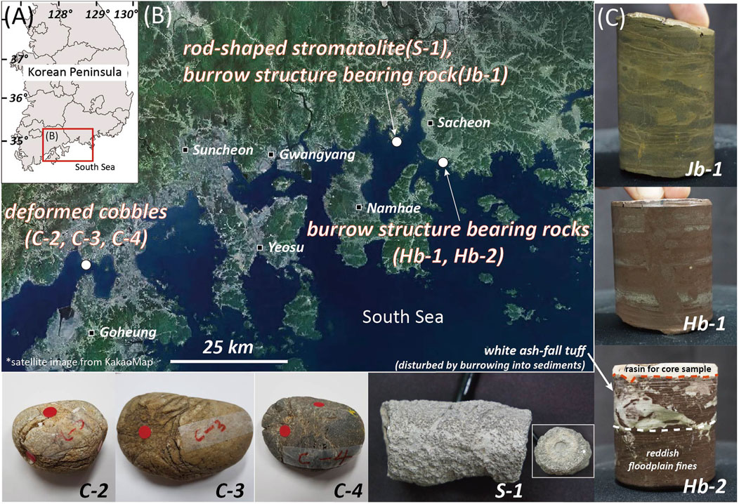
Figure 1. (A) Index map showing the Korean Peninsula with latitude and longitude coordinates. The red box indicates the area displayed in (B). (B) Sample locations in a satellite map (KakaoMap; https://map.kakao.com). Samples S-1 and Jb-1 were collected from the Bito-ri area of Sacheon-si; Hb-1 and Hb-2 from the Namildae area of the same city; and C-2, C-3, and C-4 from the Annam-ri area of Goheung-gun. (C) Photographs of collected samples. Hb-2 shows a red dashed line marking the boundary between the epoxy resin and the sample, and a white dashed line indicating the contact between the underlying floodplain fines and the overlying ash-fall tuff. The inset in S-1 displays a side view of the sample. Red stickers on C-2, C-3, and C-4 indicate areas of concentrated external deformation on the deformed cobbles. Scale reference: core samples have a diameter of approximately 55 mm, the S-1 sample is about 6.5 cm in length, and the red sticker has a diameter of 9 mm.

It is known that RSSs are rarely found worldwide, and their origin is attributed to microorganisms inhabiting the surfaces of tree fragments (e.g., twigs) (Lee and Woo, 1996; Lee and Kong, 2004; Choi, 2007). The length of the obtained RSS is approximately 6.5 cm, with the long and short axes of its vertical oval cross-section measuring 4 cm and 3 cm, respectively (Figure 1C). To the naked eye, the internal structure of the RSS in the longitudinal section is broadly divided into three areas: 1) a dimpled, light gray core; 2) a faint, light yellowish radial fabric; and 3) an outermost gray thrombolitic layer with an irregular texture (Figures 1C, 2A). The outermost surface, which is extensively exposed, exhibits a rugged texture with significant relief due to the physico-chemical differential weathering of its constituent materials (Figures 2B,D). In a specific direction along the sample’s periphery, noticeable recessed fractures are observed, caused by the development of open fractures after deposition and subsequent differential erosion of the filling materials (Figure 2B). On the a' side of the longitudinal section, the sample appears fractured and crushed (Figure 2C). On the opposite side, where fractures are less visible, traces of crushing remain (Figure 2D). Overall, the bright, light gray regions are more susceptible to weathering, resulting in engraved textures (Figure 2). Previous RSS studies have primarily relied on 2D cross-sections; however, for a more detailed morphological analysis, it is crucial to examine the internal structure through 3D-rendered imaging.

Figure 2

Figure 2. Detailed photographs of the rod-shaped stromatolite. (A,C) Both ends of the sample, showing a depressed core and a distorted core due to fracturing. (B,D) Upper and lower parts of the sample. All images share the same scale.

The samples containing burrow structures were shaped into cylindrical forms with an approximate diameter of 55 mm to allow for comparative analysis under identical conditions (Figure 1C). Their heights are approximately 90 mm for Jb-1, 70 mm for Hb-1, and 60 mm for Hb-2. Jb-1 consists of alternating layers of gray, coarse-grained siltstone and greenish-gray, medium-grained siltstone (Figure 1C). Hb-1 is composed of multiple bedding layers and laminations exhibiting normal grading, consisting of light gray, fine-grained sand to reddish silt or clay (Figure 1C). Hb-2 consists of a reddish lower bed (floodplain fines) and an upper white bed (ash-fall tuff origin: wairakite (calcium-rich zeolite mineral) and microcrystalline quartz) (Figure 1C). Both beds show evidence of bioturbation caused by invertebrate burrowing.

The deformed cobbles from the Duwon Formation exhibit four distinct types of deformation: (1) faint contact marks, (2) pitted marks without fractures, (3) pitted marks accompanied by radial or sub-parallel fractures surrounding the pits, and (4) fractures without associated pits (Chae, 2017). Internal structure analyses were conducted on selected samples that featured pitted marks with radial or sub-parallel fractures around the pits (Figure 1C). The present study focused on the third deformation type, which includes deformed cobbles exhibiting pitted marks with surrounding radial or sub-parallel fractures (Figure 1C). Such deformed cobbles have been rarely documented worldwide (e.g., Tanner, 1963; McEwen, 1978; 1981; Ernstson et al., 2001; Mokhtari, 2014). The surface of these cobbles contains pits formed by stress exerted by adjacent cobbles after deposition. Specifically, five pitted points are observed on C-2, two on C-3, and four on C-4 (Figure 1C, red stickers). Understanding the deformation and its underlying processes requires analyzing the relationship between internal fractures and pitted points, which can be effectively achieved through 3D internal structure extraction.

3 Methods

The 3D internal structure analysis of the samples was conducted using the X-EYE PCT G3 system (SEC Co., Ltd. in Korea) installed at the Korea Institute of Civil Engineering and Building Technology (KICT). The industrial X-ray CT system comprises an X-ray source, a rotating table, and an X-ray detector (Figure 3).

Figure 3

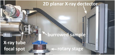
Figure 3. Laboratory-based conical X-ray micro-CT (X-EYE PCT G3 system) setup at the Korea Institute of Civil Engineering and Building Technology (KICT), consisting of an X-ray source, rotary stage, and detector. The system employs a micro-focus X-ray tube with a maximum resolution of 3.5 µm³ and operates at up to 225 kV and 3.0 mA, ensuring sufficient penetration. A CCD-based flat-panel detector (409.6 × 409.6 mm, 200 µm pixel pitch) captures X-ray attenuation data, with a limiting resolution of 2.5 lp/mm.

When the X-ray beam passes through the sample, it is absorbed and scattered based on the material’s density, with the remaining radiation reaching each pixel of the detector. At this stage, the internal structure is identified by analyzing the number of X-ray photons detected. The intensity (I) of the attenuated X-ray is expressed as follows:

$I=I_0{e}^{-\mu t}$

Where $I_0$ = irradiated X-ray intensity

$e$ = base of natural logarithm

$\mathrm{\mu }$ = linear attenuation coefficient of sample

$t$ = time

Each CT image represents a slice of the sample with thickness, composed of voxels reflecting the linear attenuation coefficient (µ), which depends on the material’s density and atomic number. These coefficients are converted into CT values, typically expressed in Hounsfield Units (HU), relative to water and air. The X-EYE system records relative X-ray intensities, which are calibrated and normalized during reconstruction to produce interpretable voxel-based images. 3D rendering of the internal structure is achieved by accumulating voxels. In this study, X-rays were generated with a tube voltage of 150 kV and a tube current of 100 µA. The spatial resolution of the voxels is 59.37 μm (unit pixel length) for S-1, Jb-1, Hb-1, and Hb-2 samples, and 84.44 μm for C-2, C-3, and C-4 samples. After correcting scanning artifacts such as cupping and ring artifacts, the 3D rendering process was performed. For internal structure analysis with volume measurement, raw data were processed using ImageJ, VGSTUDIO Max 3.1, and Avizo Fire software. Threshold segmentation was performed based on histogram contrast and voxel density in the CT images. Although precise numerical threshold values for each structure were not recorded, segmentation was conducted using manual adjustment and visual inspection to best isolate internal features. The accuracy of segmentation was validated by comparing the results with thin section observations. The internal structures observed in CT scans of RSS and sedimentary rocks containing invertebrate burrow structures were examined in greater detail through thin section analysis using a polarizing microscope. Thin sections were prepared from the same samples after X-ray CT scanning. Optical microscopy was performed using a ZEISS AXIO Lab. A1 polarizing microscope, and images were acquired with ZEN 2.3 software. No additional post-processing was applied to the images. The internal fracture patterns of the deformed cobbles were quantitatively extracted using the slicing plane method (SPM), following the statistical analysis approach proposed by Yun et al. (2013). However, for SPM to be applied, the fracture plane must span the entire analytical domain. To address this limitation, when a fracture plane was only locally present in a sample, the corresponding region was cropped to create a smaller sub-domain before applying SPM.

To understand the relationship between the extracted internal fractures and external deformation, the data were plotted on stereonets, with poles oriented perpendicular to the outer pitted surfaces. First, the coefficient of variation (Cv) values for internal fractures were represented as contoured stereonet plots. Next, the poles most parallel to the external pitted point plane were identified and overlaid on the contoured stereonet. If the normal vector at a pitted point was defined as pointing inward, it was directed toward the northern or southern hemisphere of the projection plane. For ease of analysis, the normal vectors of pitted planes projected in the opposite hemisphere to the fractures were plotted as inverse vectors, facilitating the interpretation of the directional relationship between fractures and pits.

4 Results

4.1 Rod-shaped stromatolite

4.1.1 X-ray CT images of RSS

To observe multiple cross-sections of the rod-shaped stromatolite using HRXCT, a total of 10 CT image slices were obtained at equal intervals (Figures 4A,B). The internal structure of the RSS can be broadly classified into six distinct regions, comprising two core sections and four surrounding laminations, based on variations in brightness in the CT images (Figure 4C). First, the core’s internal structure, which is not visible from the outer surface, is distinguished into two sections in the CT images (Figures 4B,C). The innermost section, “a,” is asymmetrically positioned within the core, while a brighter surrounding section, “b,” encases it (Figures 4B,C). The first surrounding lamination, “c,” is darker than section “b” and exhibits a radial fabric (Figures 4C, 5). Lamination “d” fully encloses lamination “c” and appears relatively lighter in color, with a weaker radial fabric. Lamination “e” completely encircles lamination “d” and displays a fabric similar to lamination “c,” but with more pronounced radial structures. Lastly, lamination “f,” which encloses lamination “e,” is asymmetrically distributed and features an irregular internal structure. Additionally, the volume of each internal structure was calculated. The volumes of laminations “a,” “b,” “c,” “d,” and “e + f” were measured as 600 mm³ (0.8%), 3,592 mm³ (5.1%), 2,674 mm³ (3.8%), 17,125 mm³ (24.1%), and 47,018 mm³ (66.2%), respectively. Furthermore, secondary calcite veinlets occupy approximately 1,100 mm³ (Figure 4D).

Figure 4

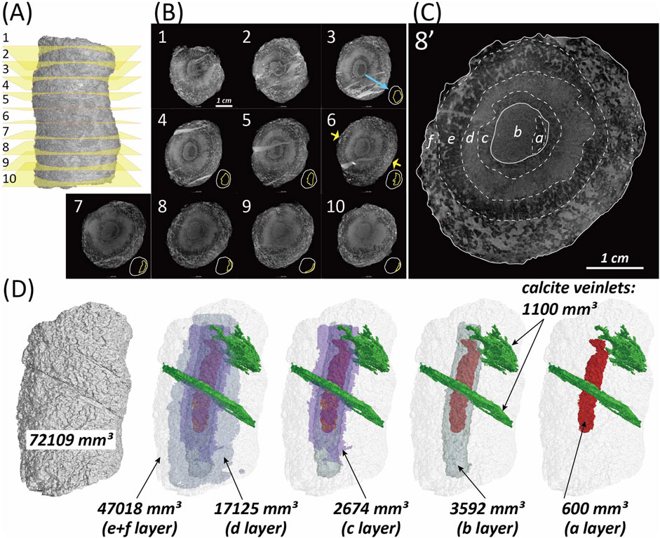
Figure 4. (A) Locations of CT slices in the rod-shaped stromatolite (RSS), corresponding to (B). (B,C) CT slices showing various internal structures. Panel (C) is an enlarged view of number 8 in (B). Detailed explanations of the labeled structures are provided in the main text. (D) Extracted 3D renderings and calculated volumes of each internal feature.

Figure 5

Figure 5. A CT slice and corresponding thin-section images under cross-polarized light (XPL) from areas (red 1, 2, and 3) marked in CT slice. Abbreviations (Yellow): F, fenestrae; BC, biogenic calcisphere; CBC, clotted biogenic calcispheres; B, biogenic fragment; MC, microfracture; DS, domal structure; CF, cyanobacterial filaments; GAF, green algal filaments.

4.1.2 Thin section analysis of RSS

Most of the core is composed of granular mosaic calcite, with residual clastic sediments distributed in certain areas (Figure 5). The overgrowth rim surrounding the core consists of biogenic calcispheres (Pithonella?), biofragments, and mud-sized clastic sediments, while fenestral and intrafossil pores are filled with micrite and microsparite (Figure 5). The composition of parts “a” to “f” is as follows:

Part “a” consists primarily of clastic sediments, while part “b” forms the remaining core material, comprising granular mosaic calcite and fragments of clastic sediments (Figure 5). Part “c” is the first layer surrounding the core, characterized by a high organic content, domal structures, and radial fenestral pores on its outer surface (Figure 5). In part “d”, the domal structure layers are slightly thicker than those in part “c”. Additionally, calcispheres and fenestral pores are more prominently developed in this region (Figure 5). Part “e” exhibits less calcisphere development compared to part “d” and primarily contains radial fenestral pores (Figure 5). Part “f”, the outermost layer of the RSS, features well-developed fenestral pores arranged in an irregular or concentric pattern, along with clotted calcispheres. Furthermore, the proportion of clastic sediments within the outer fenestral pores is significantly higher than that of the inner fenestral pores (Figure 5).

4.2 Invertebrate burrow structures

4.2.1 X-ray CT images of invertebrate burrow structures

Invertebrate burrows in the Jb-1 sample from the Jinju Formation are not clearly visible in the CT images (Figure 6A). The size and 3D shape of the burrows can be roughly identified, but their internal structures are not discernible. However, some structures exhibiting characteristics similar to Chondrites are observed (Figure 6A). In the Jinju Formation, Chondrites specimens were reported from the Dongheong section, with two representative samples collected (KNUE 990005–990006) (Kim and Pickerill, 2003). According to Kim and Pickerill (2003), Chondrites in the Jinju Formation appear as small (1–2 mm), dendritic burrows with up to three orders of asymmetric branching at angles between 31° and 71°. The Hb-1 sample exhibits slightly higher attenuation contrast than Jb-1 in the CT images (Figure 6B). Some internal structures are distinguishable within a few burrows, allowing for their classification. Some trace fossils exhibit straight to slightly curved cylindrical or semicylindrical burrows with meniscate backfill, representing successive pulses of sediment infill during movement. These features are characteristic of Taenidium, which is interpreted as a feeding trace (fodinichnion) formed by systematic sediment probing behavior (Keighley and Pickerill, 1994). However, for most burrows, only their size and 3D shape can be recognized.

Figure 6

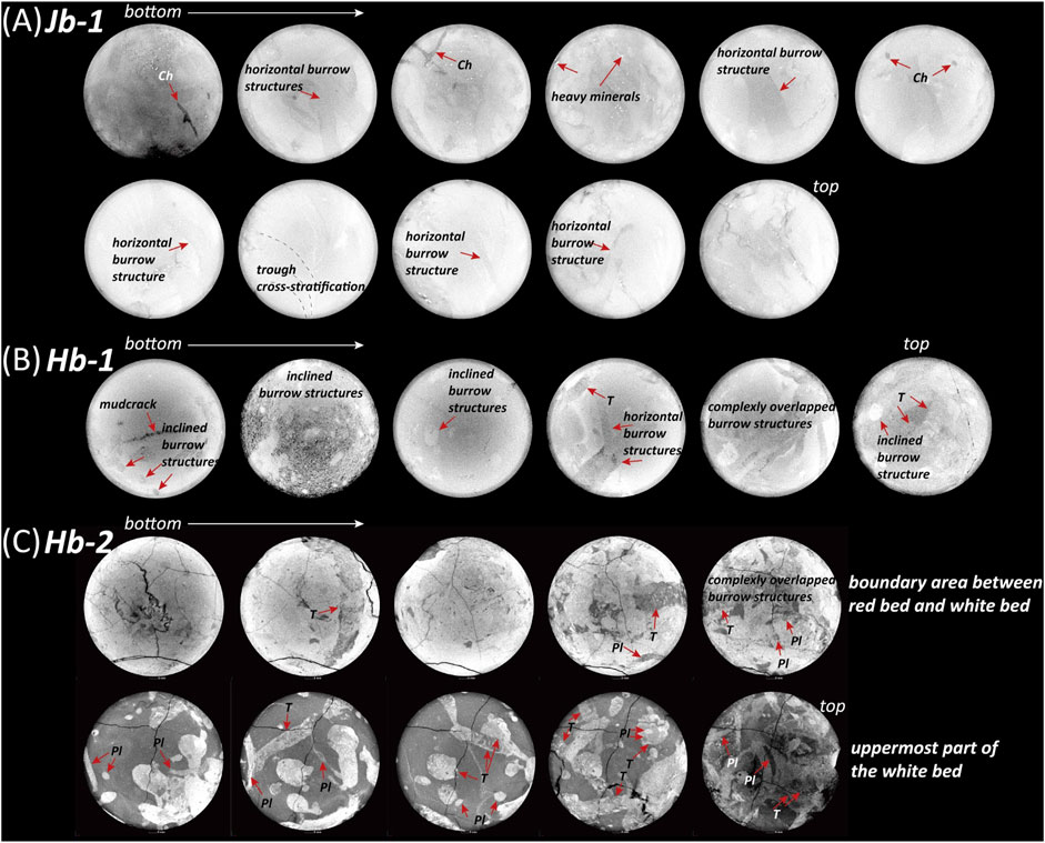
Figure 6. 2D CT slices of cylindrical rock samples containing invertebrate burrows. (A) Jb-1, (B) Hb-1, (C) Hb-2. Abbreviations: Ch, Chondrites; T, Taenidium; Pl, Planolites.

The CT images of Hb-2 show superior clarity compared to those of Jb-1 and Hb-1. Both the burrows and their internal structures are easily observable (Figure 6C). In particular, intense bioturbation is evident at the top of the white bed and along the boundary between the white and reddish beds, due to overlapping burrows and trails. Conversely, within the white bed, the burrow density is relatively low, allowing for the clear observation of individual structures. Some trace fossils exhibit unlined, simple horizontal to slightly inclined burrows filled with structureless sediment. These features are similar to Planolites reported from the Hasandong Formation by Kim and Pickerill (2003), and are interpreted as deposit-feeding traces of worms or insect larvae.

Overall, bioturbated structures were successfully extracted from Jb-1, Hb-1, and the white bed, as well as parts of the red bed in Hb-2 (Figures 7A–C). The volume extraction of the burrow structure from the Hb-2 sample was conducted only in certain section (white bed + some part of red bed) (Figure 7C). The volumes of Jb-1, Hb-1, and Hb-2 were 199,588 mm³, 161,930 mm³, and 130,164 mm³ (total for burrow extraction: 86,721 mm³), respectively. The extracted invertebrate burrow volumes were 9,419 mm³ (4.7%), 10,728 mm³ (6.6%) and 16,559 mm³ (19.1%), respectively. From the extracted 3D burrow images, most burrows are arranged parallel and/or oblique to the bedding planes, while burrows perpendicular to the planes were not observed, except for a few in Jb-1.

Figure 7

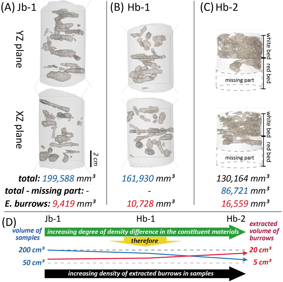
Figure 7. (A–C) Extracted 3D images and calculated volumes of invertebrate burrows, including total sample, volume excluding missing parts, and burrow volume. (D) Graph showing extracted volumes of both the sample and burrows.

4.2.2 Thin section analysis of burrow-bearing rocks

The Jb-1 sample consists of quartz-rich yellowish siltstone and mica-rich fine-grained siltstone, with interspersed secondary precipitated calcite layers within the mica-rich strata (Figure 8A). Its primary mineral components are quartz, mica, and calcite cement. The Hb-1 sample is primarily composed of reddish fine-grained siltstone and reddish medium-grained siltstone in the upper section, while the lower section contains fine-to medium-grained sandstone along with some fine- and coarse-grained siltstone (Figure 8B). Additionally, its mineral composition mainly includes quartz, feldspar, and mica, with a greater variation in particle size across layers compared to Jb-1. Furthermore, the invertebrate burrows in Hb-1 have caused significant structural disturbance. Lastly, the Hb-2 sample consists of a reddish, very fine-grained sandstone bed in the lower section and a white bed (wairakite + microcrystalline quartz) in the upper section, both of which are heavily bioturbated (Figure 8C).

Figure 8

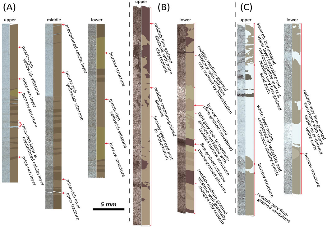
Figure 8. Line-scanned thin-section images with corresponding schematic diagrams illustrating the material composition and internal structures. (A) Jb-1 shows alternating quartz-rich yellowish siltstone, mica-rich layers, and precipitated calcite layers with a burrow structure. (B) Hb-1 is characterized by reddish fine- to medium-grained siltstone with variable clay content and extensive bioturbation. (C) Hb-2 is characterized by severely bioturbated upper layers rich in wairakite and microcrystalline quartz, grading downward into reddish very fine-grained sandstone with localized white patches.

4.3 Deformed cobbles

4.3.1 X-ray CT images of deformed cobbles

3D images of the outer surfaces and internal features of the deformed cobbles were acquired using X-ray CT (Figure 9). First, the volumes of the C-2, C-3, and C-4 cobbles were measured as 104,322 mm³, 244,942 mm³, and 142,890 mm³, respectively (Figures 9A,D,G). The corresponding volumes of internal fractures were 2,838 mm³, 1,365 mm³, and 11,998 mm³, respectively (Figures 9B,E,H). The 3D visualization of internal fractures was achieved by extracting them, revealing that their volumes account for approximately 2.72% of C-2, 0.56% of C-3, and 8.40% of C-4. The extracted 3D fracture patterns indicate that most internal fractures radiate outward from the main pits. Additionally, in the 2D CT slices, few open fractures were observed directly beneath the pitted points across all samples (Figures 9C,F,I). Notably, the development of open fractures in C-3 was minimal compared to the other samples, with only faint traces visible (Figure 9F).

Figure 9

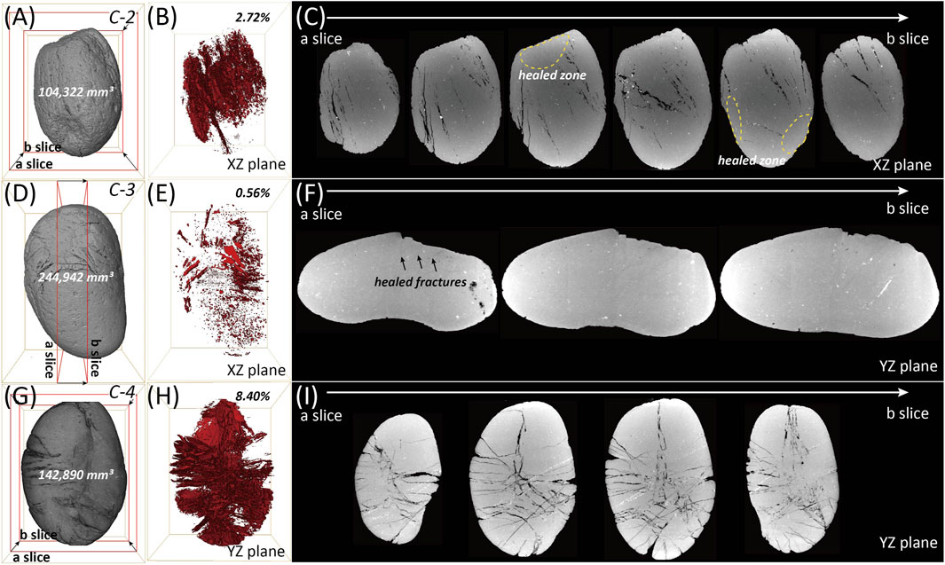
Figure 9. (A,D,G) Reconstructed 3D images of the outer surfaces of the deformed cobbles. (B,E,H) Reconstructed 3D images of internal open fractures. (C,F,I) Corresponding 2D CT slices of the cobbles.

4.3.2 Stereonet plots for outer pits and inner fractures

To determine the relationship between external pitted points and internal fractures in deformed cobbles, the data were plotted on stereonets. Because the samples were not collected with known orientations, the plots are based on an arbitrary reference frame and reflect only relative, not absolute, orientations (Figure 10). In all samples, fractures are oriented in two or more predominant directions (Figures 10D–F). The attitudes (strike/dip) of the dominant internal fracture planes extracted from the cobbles are as follows: A: 030/90 and B: 060/42 in C-2 and A1: 270/50, A2: 220/40, A3: 190/30, and B: 055/60, showing two primary fracture orientations in C-3, and A: 130/82, B: 170/90, and C: 050/40, exhibiting three dominant fracture directions in C-4 (Table 1). Additionally, the attitudes (trend/plunge) of the poles from the pitted planes are recorded as follows: 1: 300/72, 2: 056/36, 3: 254/28, 4: 114/18, 5: 333/47 in C-2, 1: 207/11, 2: 357/33 in C-3, and 1:062/36, 2: 234/30, 3: 100/00, 4: 284/02 in C-4 (Table 1).

Figure 10

Figure 10. (A–C) Extracted internal fractures and outer pits plotted on a stereonet. (D–F) Stereonets showing background contour plots for the right-angle poles of internal fractures, with white circles indicating the right-angle poles to the pitted surfaces of the cobbles.

Table 1

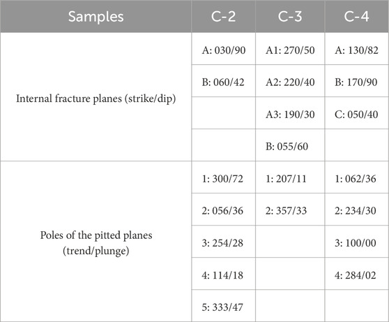
Table 1. Orientations of internal fracture planes (strike/dip) and poles of external pitted planes (trend/plunge) in deformed cobble samples C-2, C-3, and C-4. The data correspond to the stereonet plots shown in Figures 10D–F.

5 Discussion

5.1 Rod-shaped stromatolite

In the CT slice images, the bright regions represent calcareous materials, consisting predominantly of calcite with a density of 2.71 g/cm³, while the darker regions correspond to less dense detrital sediments (Figures 4B,C). Part “a” is positioned toward the right or lower right in Figure 4B, and as the section progresses from slice 3 to slice 10, the amount of residual sediment decreases, causing part “a” to change shape from elliptical to a half-moon or crescent shape (Figure 4B). This suggests that residual sediments filled the empty space left after the erosion of a tree branch during deposition. As a geopetal structure, it also serves as an indicator of the original orientation at the time of deposition. Using HRXCT, the internal structures of RSS, which exhibit multiple layers, can be extracted and visualized as 3D images for each layer (Figure 4D). Based on volume calculations, the original tree branch in S-1 is estimated to have a volume of approximately 4,192 mm³ (6% of the total), representing the combined volumes of parts “a” and “b”, while the remaining overgrowth accounts for about 94% of the total volume (Figure 4D). HRXCT offers the distinct advantage of enabling 3D visualization of internal structures and precise volume calculations without sample destruction. However, there are limitations in resolving the exact composition and fabric of the sample, as well as in identifying fine microstructures using only X-ray CT images. If a sample exhibits homogeneous fabrics or structures, as seen in RSS, information about its internal constituents can be obtained by analyzing a thin section from a portion of the sample (Figure 5). The data acquired from thin section analysis can complement the 3D images derived from X-ray CT, allowing for a more comprehensive interpretation.

5.1.1 Comparison between a CT slice image and a slab of the RSS

To evaluate how well X-ray CT captures the internal features of RSS, the actual cut surface under wet, dry, and etched conditions was compared with the corresponding CT slice image (Figure 11). Under wet conditions, domal structures and calcite veinlets within the RSS are easily observable, whereas residual clastic sediments distributed in the core are not clearly visible (Figure 11A). In contrast, under dry conditions, boundaries and domal structures are less distinct, but residual clastic sediments are more easily observed than in the wet condition (Figure 11B). When the cut surface was etched using a diluted HCl solution to slightly dissolve calcite and enhance the visibility of internal structures, the materials filling the outermost pores and the innermost part appeared bright and remained intact, indicating that they primarily consist of clastic sediments (Figure 11C). This observation is consistent with the thin section analysis shown in Figure 5. Finally, when a CT slice image corresponding to the previously analyzed cut surface was obtained, both the domal structures and residual clastic sediments were clearly distinguishable (Figure 11D). Additionally, the boundary between the branched twig and the surrounding matrix, which is difficult to discern with the naked eye, was distinctly revealed in the CT image. Therefore, CT imaging effectively simulates various internal structures observed in actual cross-sections under different conditions, providing a comprehensive and non-destructive visualization of the sample.

Figure 11

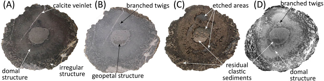
Figure 11. Comparison of photographs showing the same cross-section under different conditions. (A) Wet, (B) dry, (C) etched in diluted HCl, and (D) corresponding 2D CT slice.

5.2 Invertebrate burrow structures

The invertebrate burrow fill and the surrounding sediments primarily consist of different minerals and/or grain sizes due to the activity of invertebrates (Figure 8). This variation in composition results in differences in rock density, which are reflected in the X-ray CT images (Figure 6). In the Jb-1 and Hb-1 samples, both particle size and density exhibit minimal variation, which results in only subtle differences in grayscale values between the burrow structures and the surrounding matrix (Figures 8A,B). As a result, the approximate outlines of the burrows can be identified, but their internal structures are not clearly distinguishable, making species identification difficult (Figures 6A,B). In contrast, in the Hb-2 sample, the white bed is composed of wairakite and microcrystalline quartz (Figure 8C), with wairakite—which has a relatively low density of approximately 2.26 g/cm³—accounting for about 80% of the composition. As a result, the white bed exhibits a comparatively lower density than the red bed material, which is primarily composed of quartz and feldspar (density: approximately 2.5–2.7 g/cm³). The density difference between the burrow fills and the surrounding parent material is sufficiently large, allowing for the distinct visualization of burrow outlines and internal structures, which facilitates species identification (Figure 6C). Among the burrows in Hb-2, those lacking walls or distinct boundary lines and exhibiting a meniscate structure due to heterogeneous backfill show typical characteristics of Taenidium (Figure 6C). Additionally, some relatively small burrows with no walls, boundary lines, or internal structures can be identified as Planolites (Figure 6C). X-ray CT enables the extraction and 3D rendering of burrow structures from sedimentary rocks, providing the advantage of intuitive internal structure visualization (Figure 7). This method reveals that circular or elliptical features observed on sample surfaces with the naked eye can easily be mistaken for Skolithos; however, 3D images of internal structures confirm that most of them are actually Planolites (Figures 6C, 7C). However, if the density contrast between burrows and the surrounding material is insufficient, as in Jb-1 and Hb-1, the low contrast ratio in CT images makes it difficult to distinguish clear outlines and internal structures, thereby complicating 3D rendering of the burrow structures (Figures 6A,B, 7A,B). Consequently, although the actual burrow density in Jb-1 and Hb-1 is not significantly lower than that in Hb-2, their burrow density appears considerably lower in the 3D-rendered images (Figure 7D). Because the effectiveness of 3D visualization and extraction of internal structures using X-ray CT depends on the density contrast between constituent materials, careful consideration is necessary when extracting various sedimentary and deformed structures, including invertebrate burrows. The greater the variation in material type or size within sedimentary structures, the more advantageous X-ray CT becomes for their observation and extraction.

5.3 Deformed cobbles

Fracturing creates empty spaces, and due to the significant density difference between the parent rock and the fractures, 3D observation and rendering through CT images are relatively easy. However, in all deformed cobbles analyzed in this study, some or most of the primary fractures have been either completely erased or reduced to faint traces (Figure 9). This phenomenon occurs due to selective healing (mineral precipitation has locally sealed certain fracture pathways while others remain partially or entirely open), where secondary minerals precipitate from fluids that infiltrated the cobbles after fracturing (Figures 9C,F,I; e.g.; Jerzykiewicz, 1985). The precipitation of these secondary minerals obstructs the visibility of primary fractures in CT images. Notably, in all samples, the areas directly beneath the pitted points exhibit significant healing. Additionally, in the C-3 sample, secondary mineralization appears to have been widely distributed throughout the rock (Figures 9E,F). This secondary healing process leads to distinct differences in the fracture volume observed within the samples (Figure 9E). As a result, the calculated volumes of open fractures are often slightly or significantly smaller than their original volumes immediately after formation, with the extent of this reduction depending on the degree of secondary mineral precipitation. Furthermore, most deformed cobbles exposed at the ground surface remain relatively intact rather than separating, further indicating that fracture healing due to secondary mineral precipitation has occurred. Instead of inferring internal structures based on 2D cut surfaces, X-ray CT enables direct visualization of true 3D internal structures, allowing for both qualitative assessment and quantitative volume calculation of specific internal features within the entire sample (Figures 9B,E,H). However, when calculating the volume of specific voids in a sample using X-ray CT, the effects of secondary mineral precipitation must be considered. If the secondary minerals precipitated within fractures exhibit a significant density contrast with the host rock—despite having a smaller difference compared to void spaces—this method still holds potential for effectively applying to both qualitative and quantitative assessments of internal rock structures.

5.3.1 The relationship between pitted points and fractures

Among the two predominant sets of fractures in C-2, fractures in direction A are vertically arranged on the stereonet and appear to be primarily associated with pits 1 and 2, while fractures in set B seem to have developed due to pits 3 and 4 (Figures 10A,D). Structural analysis using stereonet and 3D CT imaging indicates that pit 1 is most closely related to the primary set A fractures. Furthermore, pit 1 exhibits the most significant visible deformation, which aligns well with the stereonet results (Figures 10D, 12A). From 2D slices and extracted 3D fractures, set A fractures predominantly develop within the cobble, while set B fractures serve as linking structures between them (Figure 12B). On the stereonet, the poles of set B fractures exhibit a distinct red-contoured tail extending toward the upper right direction (dashed arrows) from the representative yellow square point (Figure 10D). This suggests a clockwise rotation of the fractures, which is also confirmed in 2D slice images (Figure 12B). Pits 2, 3, and 4 appear to be associated with the secondary set B fractures, as indicated by the bulk analysis (Figure 10D). However, set B fractures developed differently depending on their proximity to pit 1: near pit 1, they primarily formed due to the interaction of pits 2 and 3, whereas farther from pit 1, the interaction between pits 3 and 4 became dominant (Figures 10D, 12B). Thus, the rotation of set B fractures on the stereonet is attributed to differential stresses exerted by various pits in different domains within the C-2 sample. Additionally, the white circles on the stereonet are positioned relatively far from the representative great circles (Figure 10D). This could be interpreted as the result of multidirectional stresses exerted from five different points within the sample (Figure 10A).

Figure 12

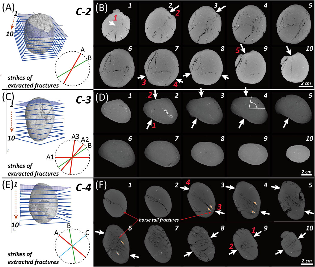
Figure 12. (A,C,E) Locations of 2D slices and strike directions of extracted representative fractures in each deformed cobble. (B,D,F) Corresponding 2D slices with arrows indicating poles of outer pits.

In the C-3 sample, very fine fractures are present, with minimal elongation and volume (Figures 9E,F, 10B). As a result, calculating specific fracture orientations may not be highly meaningful. Nevertheless, two fracture sets were identified and extracted (Figure 10E). Set A fractures predominantly develop subparallel to the XY plane and represent the primary fracture set associated with pits 1 and 2 (Figure 10E). This set, which includes A1, A2, and A3, reflects the rotation or undulation of fractures (Figure 12D). On the stereonet, fractures in set A exhibit strikes between 190° and 270°, with dips consistently to the right-hand side of strike (Figure 10E). These fractures, primarily induced by pits 1 and 2, are also visible in 2D slices (Figure 12D). Conversely, set B fractures are extremely fine, near-vertical fracture fragments that appear faintly at both ends of the sample, even in 2D slice images. In the C-3 sample, a substantial portion of the fractures underwent healing during diagenesis following the formation of the primary fractures. It is likely that the original orientation and distribution of the primary fractures were altered during the extraction process due to the effects of secondary healing. Consequently, the ∼135° trending fractures observed in slices 1 and 2 of Figure 12D were not extracted. Thus, when extracting and analyzing fractures in a given sample, the potential distortions caused by secondary healing must be carefully considered.

Unlike the previous two samples, three distinct fracture sets are observed in C-4 (Figure 10F). First, set C fractures generally exhibit a low-angle orientation relative to the stereonet plane and tend to be more diffusely distributed compared to set A and B fractures. Additionally, set C primarily consists of fractures extending across the short axis of the sample and appears to have formed under the combined influence of pits 1, 2, 3, and 4, resulting in highly undulating fracture patterns (Figures 12E,F). Analysis of 2D slices 1 through 7 of C-4 in Figure 12F reveals that set A fractures represent the dominant fractures, extending across the entire sample along the long axis. In contrast, set B fractures primarily function as connecting structures between set A fractures or resemble horsetail fractures, without crossing the entire sample (Figure 12F). These fractures can be interpreted as secondary tension fractures resulting from the dextral movement of set A fractures (Figure 12F; e.g.; Granier, 1985). The external pits most closely associated with set A fractures are pits 3 and 4, which contributed to the development of both set A and B fractures by applying stress at specific points (Figure 12F).

The above analyses represent the bulk anisotropy of the deformed cobbles. The relationship between locally applied external stress and internal fractures can be examined in greater detail through 3D image analysis (Figures 9, 10). Additionally, 3D image analysis provides the advantage of obtaining quantitative anisotropic data of the internal structure while simultaneously enabling intuitive visualization of the rendered 3D internal structure alongside the quantitative data (Figure 9). Furthermore, this approach eliminates the risk of acquiring distorted data or generating 3D images based on limited 2D observations from destructive cross-sectional analysis.

6 Conclusion

A case study utilizing HRXCT for non-destructive internal structure analysis was conducted on rod-shaped stromatolites, invertebrate burrows, and deformed cobbles found in sedimentary rocks. This method enables precise volume calculations of both entire samples and their internal structures. Additionally, HRXCT allows for the high-resolution 3D visualization of internal structures without sample destruction, offering a significant advantage over conventional destructive 2D sectioning, which provides only limited images. Furthermore, specific internal structures of interest can be selectively reconstructed and examined without interference from surrounding materials. However, resolution varies depending on the material composition and size of the sample, and there is a limitation in analyzing very large samples using HRXCT. For internal fabrics, constituent minerals, or extremely small structures that are difficult to resolve in HRXCT images, complementary observations through 2D sections, including thin sections, can provide additional insights. In particular, HRXCT offers a unique advantage in that it can replace multiple conventional analytical procedures such as observations under dry and wet conditions, etching, and thin sectioning thereby significantly reducing the time, cost, and sample preparation requirements associated with traditional methods. HRXCT analysis is applicable to a wide range of geological samples and should be widely utilized as a powerful tool for investigating internal structures in geosciences, with further potential for integration with AI-based segmentation techniques, though this requires additional investigation.

Data availability statement

The original contributions presented in the study are included in the article/supplementary material, further inquiries can be directed to the corresponding author.

Author contributions

Y-UC: Software, Data curation, Writing – original draft, Methodology. S-SK: Validation, Writing – review and editing. SH: Writing – review and editing, Methodology, Investigation. YJ: Writing – review and editing, Supervision. HL: Funding acquisition, Writing – review and editing, Conceptualization, Project administration, Supervision.

Funding

The author(s) declare that financial support was received for the research and/or publication of this article. This study was funded by the National Research Foundation of Korea (NRF) grant funded by the Korean Government (2023R1A2C1006945, RS-2024-00337235).

Acknowledgments

We thank Prof. Kyung Soo Kim (Chinju National University of Education) and Prof. Cheong-Bin Kim (Sunchon National University) for their assistance with the field survey.

Conflict of interest

The authors declare that the research was conducted in the absence of any commercial or financial relationships that could be construed as a potential conflict of interest.

Generative AI statement

The author(s) declare that no Generative AI was used in the creation of this manuscript.

Any alternative text (alt text) provided alongside figures in this article has been generated by Frontiers with the support of artificial intelligence and reasonable efforts have been made to ensure accuracy, including review by the authors wherever possible. If you identify any issues, please contact us.

Publisher’s note

All claims expressed in this article are solely those of the authors and do not necessarily represent those of their affiliated organizations, or those of the publisher, the editors and the reviewers. Any product that may be evaluated in this article, or claim that may be made by its manufacturer, is not guaranteed or endorsed by the publisher.

References

Appoloni, C. R., Fernandes, C. P., and Rodrigues, C. R. O. (2007). X-ray microtomography study of a sandstone reservoir rock. Nucl. Instrum. Methods Phys. Res. Sect. A Accel. Spectrom. Detect. Assoc. Equip. 580, 629–632. doi:10.1016/j.nima.2007.05.027

CrossRef Full Text | Google Scholar

Bultreys, T., Boone, M. A., Boone, M. N., De Schryver, T., Masschaele, B., Van Hoorebeke, L., et al. (2016). Fast laboratory-based micro-computed tomography for pore-scale research: illustrative experiments and perspectives on the future. Adv. Water Resour. 95, 341–351. doi:10.1016/j.advwatres.2015.05.012

CrossRef Full Text | Google Scholar

Caso, F., Petroccia, A., Nerone, S., Maffeis, A., Corno, A., and Zucali, M. (2024). Comparison between 2D and 3D microstructures and implications for metamorphic constraints using a chloritoid–garnet-bearing mica schist. Eur. J. Mineralogy 36 (3), 381–395. doi:10.5194/ejm-36-381-2024

CrossRef Full Text | Google Scholar

Chae, Y.-U. (2017). Classification and formation mechanism of deformed cobbles from the Early Cretaceous duwon formation, goheung basin. Busan, Korea: Pusan National University, 104. MS Thesis.

Google Scholar

Choi, C. G. (2007). Rod-shaped stromatolites from the jinju formation, sacheon, gyeongsangnam-do, Korea. J. Korean Earth Sci. Soc. 28, 54–63. doi:10.5467/JKESS.2007.28.1.054

CrossRef Full Text | Google Scholar

Cnudde, V., and Boone, M. N. (2013). High-resolution X-ray computed tomography in geosciences: a review of the current technology and applications. Earth-Science Rev. 123, 1–17. doi:10.1016/j.earscirev.2013.04.003

CrossRef Full Text | Google Scholar

Ernstson, K., Rampino, M. R., and Hiltl, M. (2001). Cratered cobbles in Triassic buntsandstein conglomerates in northeastern Spain: an indicator of shock deformation in the vicinity of large impacts. Geology 29, 11–14. doi:10.1130/0091-7613(2001)029<0011:ccitbc>2.0.co;2

CrossRef Full Text | Google Scholar

Granier, T. (1985). Origin, damping, and pattern of development of faults in granite. Tectonics 4 (7), 721–737. doi:10.1029/tc004i007p00721

CrossRef Full Text | Google Scholar

Heřmanová, Z., Bruthansová, J., Holcová, K., Mikuláš, R., Veselská, M. K., Kočí, T., et al. (2020). Benefits and limits of x-ray micro-computed tomography for visualization of colonization and bioerosion of shelled organisms. Palaeontol. Electronica 23 (2), a23. doi:10.26879/1048

CrossRef Full Text | Google Scholar

Hipsley, C. A., Aguilar, R., Black, J. R., and Hocknull, S. A. (2020). High-throughput microCT scanning of small specimens: preparation, packing, parameters and post-processing. Sci. Rep. 10 (1), 13863. doi:10.1038/s41598-020-70970-7

PubMed Abstract | CrossRef Full Text | Google Scholar

Jerzykiewicz, T. (1985). Tectonically deformed pebbles in the brazeau and paskapoo formations, central Alberta foothills, Canada. Sediment. Geol. 42, 159–180. doi:10.1016/0037-0738(85)90043-0

CrossRef Full Text | Google Scholar

Keighley, D. G., and Pickerill, R. K. (1994). The ichnogenus beaconites and its distinction from ancorichnus and taenidium. Palaeontology 37 (2), 305–337.

Google Scholar

Kim, J. Y., and Pickerill, R. K. (2003). Cretaceous nonmarine trace fossils from the hasandong and jinju formations of the namhae area, kyongsangnamdo, southeast Korea. Ichnos 9, 41–60. doi:10.1080/10420940190034076

CrossRef Full Text | Google Scholar

Lee, S. J., and Kong, D. (2004). Rod-shaped stromatolites from the jinju formation, namhae, Gyeongsangnam-do, Korea. J. Geol. Soc. Korea 40, 13–26.

Google Scholar

Lee, K. C., and Woo, K. S. (1996). Lacustrine stromatolites and diagenetic history of carbonate rocks of chinju formation in kunwi area, kyongsangbukdo, Korea. J. Geol. Soc. Korea 32, 351–365.

Google Scholar

McEwen, T. J. (1978). Diffusional mass transfer processes in pitted pebble conglomerates. Contributions Mineralogy Petrology 67, 405–415. doi:10.1007/BF00383300

CrossRef Full Text | Google Scholar

McEwen, T. J. (1981). Brittle deformation in pitted pebble conglomerates. J. Struct. Geol. 3, 25–37. doi:10.1016/0191-8141(81)90054-7

CrossRef Full Text | Google Scholar

Mees, F., Swennen, R., Van Geet, M., and Jacobs, P. (2003). Applications of X-ray computed tomography in the geosciences. J. Geol. Soc. 215. doi:10.1144/GSL.SP.2003.215.01.01

CrossRef Full Text | Google Scholar

Mokhtari, A. (2014). Evidence of shock metamorphism effects in suevite from the triffa plain in north eastern Morocco. Univers. J. Appl. Sci. 2, 77–82. doi:10.13189/ujas.2014.020402

CrossRef Full Text | Google Scholar

Racicot, R. (2016). Fossil secrets revealed: X-ray CT scanning and applications in paleontology. Paleontol. Soc. Pap. 22, 21–38. doi:10.1017/scs.2017.6

CrossRef Full Text | Google Scholar

Reid, M., Bordy, E. M., Taylor, W. L., le Roux, S. G., and du Plessis, A. (2019). A micro X-ray computed tomography dataset of fossil echinoderms in an ancient obrution bed: a robust method for taphonomic and palaeoecologic analyses. GigaScience 8, giy156. doi:10.1093/gigascience/giy156

PubMed Abstract | CrossRef Full Text | Google Scholar

Sutton, M. D. (2008). Tomographic techniques for the study of exceptionally preserved fossils. Proc. R. Soc. Lond. B. Biol. Sci. 275 (1643), 1587–1593. doi:10.1098/rspb.2008.0263

PubMed Abstract | CrossRef Full Text | Google Scholar

Tanner, W. F. (1963). Crushed pebble conglomerate of Southwestern Montana. J. Geol. 71, 637–641. doi:10.1086/626937

CrossRef Full Text | Google Scholar

Wildenschild, D., and Sheppard, A. P. (2013). X-ray imaging and analysis techniques for quantifying pore-scale structure and processes in subsurface porous medium systems. Adv. Water Resour. 51, 217–246. doi:10.1016/j.advwatres.2012.07.018

CrossRef Full Text | Google Scholar

Withers, P. J., Bouman, C., Carmignato, S., Cnudde, V., Grimaldi, D., Hagen, C. K., et al. (2021). X-ray computed tomography. Nat. Rev. Methods Primers 1 (1), 18.

Google Scholar

Yun, T. S., Jeong, Y. J., Kim, K. Y., and Min, K.-B. (2013). Evaluation of rock anisotropy using 3D X-ray computed tomography. Eng. Geol. 163, 11–19. doi:10.1016/j.enggeo.2013.05.017

CrossRef Full Text | Google Scholar

Zhang, P., Lee, Y. I., and Zhang, J. (2019). A review of high-resolution X-ray computed tomography applied to petroleum geology and a case study. Micron 124, 102702. doi:10.1016/j.micron.2019.102702

PubMed Abstract | CrossRef Full Text | Google Scholar