Inverse geo-electromagnetic modeling: a systematic review and bibliometric assessment

Inverse electromagnetic (EM) modeling plays a pivotal role in subsurface exploration, enabling the characterization of the Earth’s electrical properties for various applications, including resource exploration, environmental monitoring, and geohazard assessment. Despite significant advancements in the field, the EM inverse problem remains inherently challenging due to its ill-posed and nonlinear nature. A diverse range of methodologies, including deterministic, non-deterministic, and machine learning-based (ML-based) approaches, have been proposed to address these challenges. However, there is a lack of a comprehensive synthesis that integrates both the theoretical evolution of these methods and their bibliometric performance. This paper addresses this gap by combining a systematic review of modern computational methodologies with a bibliometric assessment of the scientific literature on inverse EM modeling. The systematic review critically evaluates key computational approaches, examining their theoretical foundations, practical applications, and limitations, while the bibliometric assessment provides a quantitative assessment of scientific productivity, trends, and contributions from different nations. This integrated perspective offers a unified overview of the field, identifies emerging research directions, and highlights the state-of-the-art in inverse EM modeling. The findings provide valuable insights for researchers, practitioners, and policymakers, guiding future advancements and fostering interdisciplinary collaboration.

Highlights

i. Provides a comprehensive synthesis of inverse EM modeling by combining systematic review methodologies with bibliometric assessment

ii. Examines deterministic, stochastic, and ML-based approaches, critically evaluating their applicability, advantages, and limitations in geophysical exploration

iii. Identifies key global contributions, thematic evolution, and future research directions through quantitative bibliometric techniques and unsupervised neural networks

iv. Enhances geophysical imaging strategies for mineral exploration, groundwater assessment, hydrocarbon detection, and environmental monitoring.

1 Introduction

Inverse electromagnetic (EM) modeling is an essential tool in subsurface exploration, facilitating the characterization of the Earth’s electrical properties for applications such as resource exploration (Newman and Alumbaugh, 1997; Eidesmo et al., 2002; Avdeev, 2005; Constable, 2006; Srnka et al., 2006; Orange et al., 2009; Constable, 2010; Castillo-Reyes et al., 2018; Werthmüller et al., 2021), mineral and resource mining (Sheard et al., 2005; Queralt et al., 2007; Yang and Oldenburg, 2012), ${\text{CO}}_2$ storage characterization (Girard et al., 2011; Vilamajó et al., 2013), geothermal reservoir imaging and characterization (Piña-Varas et al., 2015; Coppo et al., 2016), crustal conductivity studies (Hördt et al., 1992; Hördt et al., 2000; Ledo et al., 2002; Campanyà et al., 2012), and hydrogeological (Chambers et al., 2006; Chang et al., 2017; Zhang et al., 2016). Among its key techniques, inverse EM modeling stands out for its ability to reconstruct subsurface conductivity structures from observed EM field data. However, the EM inverse problem is inherently challenging due to its ill-posed and nonlinear nature, necessitating the development of sophisticated computational and algorithmic approaches. Over the years, EM community have proposed a broad spectrum of methodologies, including deterministic, non-deterministic, machine learning-based (ML-based) schemes, and deep learning-based (DL-based) techniques, to address these challenges. Despite this progress, the field lacks a cohesive synthesis of its evolution, trends, and future directions, making it difficult to identify critical knowledge gaps and prioritize areas for further research.

Previous works have explored various facets of inverse EM modeling (Etgen et al., 2009; Zhdanov, 2010; Newman, 2014; Sun et al., 2022; Heagy et al., 2017; Xue et al., 2020; Wagner and Uhlemann, 2021; Wang et al., 2021; Castillo-Reyes et al., 2023a; Castillo-Reyes et al., 2024). Earlier studies primarily focused on deterministic methods, emphasizing their mathematical rigor and suitability for well-constrained scenarios but also highlighting their sensitivity to noise and limitations in handling complex geological structures (Xue et al., 2020). Subsequent works expanded the scope to include non-deterministic approaches, such as stochastic and probabilistic methods, which introduced uncertainty quantification (Ernst et al., 2020) and demonstrated robustness in handling ill-posed problems (Gunning et al., 2010; Mittet and Morten, 2012; Zhang et al., 2020). More recently, the integration of ML techniques has attracted significant attention, with works discussing their potential to process large datasets, identify patterns, and accelerate EM inversion workflows (Kim and Nakata, 2018; Puzyrev, 2019; Russell, 2019; Ma et al., 2024; Schuster et al., 2024). Despite these contributions, existing reviews tend to concentrate on specific methodologies or application areas, lacking a holistic perspective that encompasses both theoretical advancements and bibliometric insights (Donthu et al., 2021) into the field’s evolution. This gap underscores the need for a comprehensive analysis that integrates systematic and bibliometric approaches to provide a broader understanding of inverse EM modeling.

This paper addresses this need by integrating a systematic review of modern computational methodologies with a bibliometric assessment of the scientific literature in inverse EM modeling. The systematic review provides a critical evaluation of the primary approaches employed in the field, highlighting their theoretical underpinnings, practical applications, and inherent limitations. Simultaneously, the bibliometric assessment offers a quantitative perspective on the field’s development, examining trends in scientific productivity, contributions from different nations, and the thematic evolution of research. Together, these complementary methodologies present a comprehensive view of the field, bridging the gap between qualitative insights and quantitative analysis. The novelty of this study lies in its ability to provide an integrated perspective that combines theoretical analysis with bibliometric evaluation. While previous relevant studies often focus on isolated aspects, such as algorithmic and numerical advancements or specific application fields, this paper offers a unified overview that contextualizes the field’s historical development and identifies emerging opportunities. By integrating qualitative and quantitative insights, this paper highlights the state-of-the-art in inverse EM modeling while setting the stage for future research and interdisciplinary collaboration. It serves as a valuable resource for researchers and practitioners, addressing existing challenges and uncovering emerging opportunities in the field.

The paper is organized as follows. Section 2 details the methodology for conducting the systematic review and bibliometric assessment. Section 3 establishes the theoretical foundation of direct and inverse EM modeling. Section 4 presents the systematic review, classifying computational approaches into deterministic, non-deterministic, and ML methods while discussing their respective contributions and limitations. Section 5 reports the bibliometric assessment, highlighting trends in scientific performance, national contributions, and the thematic structure of the research field. Finally, Section 6 concludes with a summary of findings, their implications, and proposed directions for future research.

2 Methodology

In this section, we outline the methodological approach used to conduct the literature review (Table 1 provides a summary of the reviewed literature). Our methodology includes two key components: a systematic review and a bibliometric assessment. The systematic review was used to identify, select, and critically evaluate relevant studies, ensuring a thorough examination of existing research. Following this, a bibliometric assessment was performed to quantitatively assess the research landscape, offering insights into publication trends, influential works, and collaborative networks within the field. Together, these methodologies provide a robust framework for synthesizing current knowledge and identifying future research directions. Below, we detail each component.

Table 1

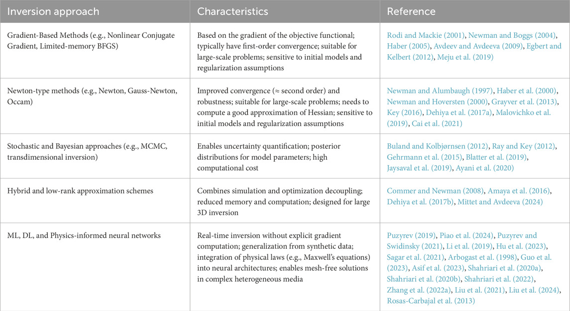
Table 1. Overview of key inversion methods in EM modeling, their main characteristics, and representative works.

2.1 Systematic review component

Inspired by Grant and Booth (2009); Paré and Kitsiou (2017), we followed a comprehensive and rigorous process to identify and select relevant papers and studies for this literature review. Multiple academic and institutional databases were searched to ensure wide literature coverage. Carefully chosen search terms encompassed various aspects of direct and inverse EM modeling. Initially, broad terms were used, and then refined using Boolean operators to increase result specificity. To ensure the quality and relevance of the selected literature, we applied strict inclusion and exclusion criteria (Rosenthal and DiMatteo, 2001). Inclusion criteria involved peer-reviewed journal articles, conference papers, and book chapters published within the last five decades. The studies had to focus on EM inverse modeling assessment methodologies and/or their applications in real-world case studies. Purely theoretical studies without practical applications and studies with insufficient data were excluded. Despite rigorous efforts to include all relevant literature, the review process may be affected by limitations and potential biases (Green and Hall, 1984). These biases could arise due to the search strategy’s reliance on specific keywords and the use of selected databases, which might inadvertently lead to the exclusion of some pertinent papers. Additionally, there is a possibility of publication bias, where studies with statistically significant findings are more likely to be included in the review. To address these bias issues, a comprehensive search strategy was implemented using specialized databases renowned for their extensive coverage of scientific literature. The search strategy was carefully designed, incorporating relevant keywords related to EM inverse modeling, EM scattering, and associated methodologies. The use of Boolean operators AND and OR effectively combined these terms to maximize the retrieval of relevant studies. Furthermore, we critically examines studies that demonstrate high-quality methodologies, sound data validation, and reliable results, thus minimizing the impact of publication bias. During the data extraction process, a systematic review approach was adopted. Pertinent information, including type of EM inverse modeling schemes, employed methodologies, and case study details, was meticulously extracted and organized into a standardized data extraction form. To ensure the quality and reliability of the studies, a thorough quality assessment was conducted. This assessment evaluated the robustness of the methodologies employed, the validity of data sources used, and the coherence of the findings reported.

Finally, we give particular attention to seminal works and influential papers that have made significant contributions to the field under consideration. Here, we highlight key methodological advancements, novel approaches, and innovative ideas presented in those papers, demonstrating their profound influence on the development of research in this domain. We also delve into an in-depth analysis of validation techniques used to assess the accuracy and reliability of EM inverse modeling. By incorporating case studies from diverse geographic regions and hazard types, we thoroughly evaluate the practical application of these methods and the effectiveness of EM inverse modeling strategies implemented based on the assessment outcomes.

2.2 Bibliometric review component

The rationale for employing a bibliometric approach stems from the goal of conducting a comprehensive literature review on EM imaging inversion methods and addressing pertinent questions within the academic community. For instance, what are the primary topics examined in this field? Which countries are most active in this research? Which agencies predominantly fund these studies? To investigate these questions, we utilize a bibliometric methodology enhanced by unsupervised artificial neural networks (ANN) and various visual analytic tools. Therefore, in order to complement the systematic review component with a general analysis and visualizations of the EM inverse modeling domain, we followed well established methodologies of science mapping developed in the fields of bibliometrics and scientometrics, science of science (Fortunato et al., 2018) or we can also call it: Meta-Science. The main goals are twofold. Firstly to quantitatively assess the bibliometric performance of the EM inverse modeling domain, and secondly to describe its scientific structure and trends, using scientific and technological information. To accomplish our first goal, we follow the methodologies developed by Villaseñor et al. (2017); Jiménez-Andrade (2023); Ruiz-Sánchez et al. (2024) and for the analysis and visualization of the landscape EM inverse modeling, we use author keywords co-occurrence networks (Radicchi et al., 2012).

Bibliometric indicators are commonly used to assess research output, though they are not without controversy (Moed, 2002). Despite these concerns, bibliometric scholars have consistently emphasized the importance of using multiple indicators to capture the various dimensions of academic activity (Moed, 2017). However, comparing units of analysis characterized by more than three indicators presents significant challenges. To address this, we employ ANN. The Self-Organizing Map (SOM) is an ANN that is based on competitive and unsupervised learning. It was first proposed by Kohonen (1981), Kohonen (1982) as a visualization tool and later revisited in by Kohonen (2001), Kohonen (2013). It is mainly used for visualization and clustering of multidimensional data and it constitutes one powerful data mining technique. In the context of the bibliometric assessment the goal is to discover some underlying structure of the data by a non linear dimensionality reduction method. SOM clusters data such that of the statistical relationships between multidimensional data are converted into a much lower dimensional latent space that preserves the geometrical relationships among the data points. SOMs provide a very powerful tool to visualize multidimensional data in a 2-D retina that gives us the possibility to see hidden interrelationships among the data.

Scientific papers are associated with other papers by means of citation in their bibliography or in the footnotes. Thus, bibliographic data can be naturally represented by complex networks. An important use of these networks is to describe scientific structure and trends of a given field such EM inversion. For this purpose, concurrence networks, are commonly employed in bibliometric reviews and they provide a visual representation of relationships between concepts, terms, or entities within academic literature. These networks facilitate the identification of patterns, connections, and clusters within a research domain. For instance, a co-occurrence network illustrates how frequently two entities, such as keywords, authors, or publications, appear together in a dataset. Such networks are instrumental in understanding popular topics, emerging trends, and thematic groupings within specific fields of study (e.g., van Eck and Waltman, 2014; Newman, 2001). To illustrate the author keyword co-occurrence we have included a network on Figure 5. To carry out the multidimensional analysis of bibliometric profiles we used the software tool LabSOM (Jiménez-Andrade et al., 2020) and for the citation networks analysis we used VoSViewer (Eck and Waltman, 2010).

3 Theory

Generating accurate EM subsurface images requires addressing both the direct and inverse problems. The direct EM problem, or forward problem, involves simulating EM responses at various receiver locations based on a known survey setup and subsurface resistivity distribution. In contrast, the inverse problem seeks to refine an initial subsurface model by minimizing misfit between measured and forward-modeled data. This refinement is achieved through iterative adjustments to the initial model using optimization algorithms until the direct problem responses closely match the measured data. This iterative procedure arises due to the non-linear nature of the EM inverse problem.

The general relationship between the forward problem and inverse problem, as depicted in Figure 1, can be schematically represented by the following diagram.

$\text{Forward\hspace{0.17em}problem:\hspace{0.17em}}{\mathbf{d}}^{\mathit{mod}}=A_s(\mathbf{m}),(1)$

$\text{Inverse\hspace{0.17em}problem:\hspace{0.17em}}\mathbf{m}=A_s^{-1}({\mathbf{d}}^{\mathit{obs}}),(2)$

where ${\mathbf{d}}^{\mathit{mod}}$ and ${\mathbf{d}}^{\mathit{obs}}$ are modeled/simulated and observed data (EM responses), respectively, $\mathbf{m}$ is the model parameters, $A_s$ denotes the forward problem operator corresponding to a source $s$, and $A_s^{-1}$ is the inverse problem operator. In this scenario, it is assumed that the parameters associated with source $s$ are known. The inverse problem associated with Equation 2, when applied to EM or acoustic field propagation, is commonly referred to as the inverse scattering problem.

Figure 1

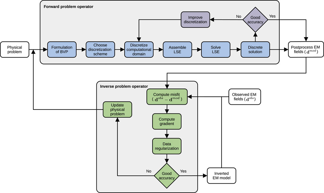
Figure 1. Schematic representation of the relationship between the forward and inverse problems.

The theoretical basis for studying EM responses, as investigated by the geophysical community through active-source methods like controlled-source EM (CSEM) techniques and passive-source methods such as magnetotelluric (MT) approaches, operates under the assumption of negligible displacement currents. In this context, assuming time-dependent variation as $e^{i\omega t}$, Maxwell’s equations considered within the frequency domain (Stratton, 2007).

$\nabla \times \mathbf{E}=-i\omega \mu \mathbf{H},(3)$

$\nabla \times \mathbf{H}=\sigma \mathbf{E}+{\mathbf{J}}_s,(4)$

$\nabla \cdot \mathbf{H}=0,(5)$

$\nabla \cdot \mathbf{E}=0,(6)$

where $\mathbf{E}$ is the electric field, $\mathbf{H}$ is the magnetic field, $i$ is the imaginary unit, $\omega$ is the angular frequency of the EM wave, $\mu$ is the magnetic permeability, $\sigma$ is the electric conductivity of the medium, and ${\mathbf{J}}_s$ is the current density due to source. Note that when MT methods are used, the natural electric and magnetic fields of the Earth’s subsurface are measured, and no external sources are generated, so ${\mathbf{J}}_s=0$.

Based on the previously defined Maxwell’s equations, the EM properties of the media are characterized by two parameters: electric conductivity ($\sigma$) and magnetic permeability ($\mu$). Consequently, the forward problem operator $A_s$, can be described as follows

$\{\mathbf{E},\mathbf{H}\}=A_s\{\sigma ,\mu \}.(7)$

For simple 1D models, there exist analytical or semi-analytical solutions for Equation 7. For 2D and 3D models, the solutions are approximated numerically, thus a discrete formulation of the boundary value problem (BVP) is required. Several numerical schemes for solving this BVP have been developed. These numerical developments are based on four major strategies: finite differences (FD; Mackie et al., 1994; Newman and Alumbaugh, 2002; Davydycheva et al., 2003; Dehiya, 2021), finite volumes (FV; Hermeline, 2009; Jahandari and Farquharson, 2014), finite elements (FE; Key and Ovall, 2011; Um et al., 2013; Jin, 2015; Rivera-Rios et al., 2019; Castillo-Reyes et al., 2019), and integral equations (IE; Raiche, 1974; Wannamaker et al., 1984; Wannamaker, 1991; Xiong and Tripp, 1997). We refer to Avdeev et al. (2002), Avdeev (2005), Börner (2010), Castillo-Reyes et al. (2024) for comprehensive reviews of numerical scheme developments for EM forward modeling.

With the discrete equations, one can obtain a linear system of equations (LSE) of the form $\mathbb{A}\mathit{x}=\mathit{b}$, where $\mathbb{A}$ is the matrix defined by the input resistivity model and mesh discretization (e.g., FD, FV, FE, IE), $\mathit{x}$ is the vector of unknown EM fields or degrees of freedom (dof), and $\mathit{b}$ is given by the source term $s$ (e.g., total field (Zhdanov, 2009) or electric field decomposition (Castillo-Reyes et al., 2018)) and boundary conditions (e.g., dirichlet conditions (Cai et al., 2017; Castillo-Reyes et al., 2018) or perfectly matched layers (Park et al., 2008; Li et al., 2018)). Note that matrix $\mathbb{A}$ is sparse, complex, and symmetric for FD, FV, and FE formulations. For IE-based solutions, $\mathbb{A}$ is dense, complex, and symmetric.

The resulting LSE can be solved either iteratively or directly, with both methods exhibiting comparable memory demands and convergence rates. Once the solution is obtained, the forward EM responses are post-processed at specified locations of interest (e.g., receiver locations). To assess the accuracy of the EM forward responses, they can be compared against a reference solution or evaluated using error estimation techniques (Grayver et al., 2013; Grayver and Bürg, 2014). Additionally, to enhance the precision of the EM responses, the model discretization can be refined through the application of tailored gridding strategies (Plessix et al., 2007; Spitzer, 2022; Castillo-Reyes et al., 2023b).

In contrast, the inverse problem in EM applications entails determining the EM properties of the medium, specifically the electrical conductivity ($\sigma$) from the observed EM fields $\mathbf{E}$ and $\mathbf{H}$. Consequently, the inverse problem operator $A_s^{-1}$ can be expressed as follows

$\{\sigma ,\mu \}=A_s^{-1}\{\mathbf{E},\mathbf{H}\}.(8)$

This inverse problem is inherently nonlinear, making the inversion of EM data a complex and challenging task in geophysics, as it requires addressing three fundamental questions: Does a solution exist? Is the solution unique? Is the solution stable? These inquiries have driven extensive research into the formulation of inverse problems with respect to these criteria. Specifically, an inverse problem is considered well-posed if its solution exists, is unique, and is stable. Within the EM context, this subject has been extensively studied by O’Sullivan (1986), Tarantola and Valette, (1982), Baumeister (1987), Sarkar et al. (1981), Groetsch and Groetsch (1993), Tarantola (2005), Alberts and Bilionis (2024).

4 Systematic literature review

4.1 Deterministic methods

Deterministic inversion is a widely used approach in geophysics for solving inverse problems, employing optimization principles. This method is intuitive and interpretable, enhancing the development of comprehensive mathematical theories for inverse modeling. Deterministic inversion modeling aims to find a model that fits the simulated data for an estimated model to the observed data. Therefore, a mechanism must be defined to evaluate the fit between simulated and observed data. In general, the observed/simulated data are finite in numbers and can be arranged in vector representation. A point-by-point difference of data points gives a misfit vector, and subsequent norms are employed to determine the misfit as a scalar. The minima of the norms can be evaluated by differentiating the norm and finding a solution where it is first derivative vanishes. The 2-norm is preferred among other norms due to its quadratic form, which leads to a linear system of equations during the optimization. A 2-norm (denoted as $|.{|}_2$) misfit functional ($\mathrm{\Phi }(\mathbf{m})$) can be written as

$\mathrm{\Phi }(\mathbf{m})=|{\mathbf{d}}^{\mathit{obs}}-{\mathbf{d}}^{\mathit{mod}}{|}_2,(9)$

The aim of inverse modeling is to evaluate model parameters, $\mathbf{m}$ by minimizing the above defined functional. As the forward modeling operator depends on the model parameter for EM modeling, minimizing the above functional is a nonlinear problem. Furthermore, it is an ill-posed problem in the case of EM data. Therefore, additional constraints are required to optimize the above functional, which is why its optimization is categorized as an inverse problem. Tikhonov and Arsenin (1977) provide a technique known as the regularization method that allows ill-posed problems to be solved. Using a Lagrange multiplier strategy, this method assembles an augmented functional by including additional constraints. A general expression for regularized objective functional can be written as

$\mathrm{\Phi }(\mathbf{m})=|\mathbf{W}({\mathbf{d}}^{\mathit{obs}}-{\mathbf{d}}^{\mathit{mod}}){|}_2+\lambda {\displaystyle \sum _{j=1}^n}{\alpha }_j|{\mathbf{L}}_j\mathbf{m}{|}_2,(10)$

where $\mathbf{W}$ is data covariance matrix, $\lambda$ denotes regularization parameter, ${\mathbf{L}}_i$ are regularization operators whose operation on model parameter, $\mathbf{m}$, imposes the additional constraints, $n$ denotes the number of regularization functional and ${\alpha }_j$ represents the weight to $j^{th}$ regularization term. It is to be noted that ${\mathbf{L}}_i$ may be designed to enforce the characteristic of prior information. In this case, its structure depends on prior information, such as a reference model. Generally, a single regularization operator ($n$ = 1) is used in EM inversion algorithms, particularly in isotropic cases.

Different optimization techniques can be used to minimize Equation 10, such as steepest descent, Levenberg-Marquart technique, non-linear conjugate gradient (NLCG (Rodi and Mackie, 2001)), Newton’s method (Haber et al., 2000) and its variants (Newman and Alumbaugh, 1997). All of these methods use the gradient of the objective functional calculated at its current position to update the model. Since the gradient points in the direction of maximum change, the reverse direction of the gradient provides the direction in which the functional reduces the most at that position. The above-listed optimization methods applied various transformations/corrections to achieve faster convergence. Therefore, a generalized expression for correction in model parameter (denoted by $\delta \mathbf{m}$) at $i^{th}$ inversion iteration can be written as

$\delta \mathbf{m}=-\mathcal{L}\nabla (\mathrm{\Phi }(\mathbf{m})),(11)$

where $\nabla (.)$ represents a gradient operation and $\mathcal{L}$ denotes transformation, which depends on the choice of the optimization method. The negative sign ensures the reversed gradient direction. The gradient of the functional given in Equation 10 can be written as

$\nabla (\mathrm{\Phi }(\mathbf{m}))=-{\mathbf{J}}^T{\mathbf{W}}^T\mathbf{W}({\mathbf{d}}^{\mathit{obs}}-{\mathbf{d}}^{\mathit{mod}})+\lambda {\displaystyle \sum _{j=1}^n}{\alpha }_j{\mathbf{L}}_j^T{\mathbf{L}}_j\mathbf{m},(12)$

where $\mathbf{J}$ is the Jacobian matrix calculated for current model parameters. The convergence of the inversion depends on the Jacobian matrix’s singular values and the optimization method. The distribution of singular values of the Jacobian determines the shape of the objective functional ($\varphi (m)$), where wider distribution causes a slow convergence. The Jacobian associated with the EM inverse problem has numerous zero singular values, which is why additional constraints are required to stabilized the solution.

In the case of the steepest descent method, $\mathcal{L}$ is a scalar, known as step length, that controls how much correction is applied using the current gradient. It is generally chosen such that the objective functional for the next updated model lies at the point where the reverse gradient tangentially touches a contour of the objective functional. The steepest descent shows a very slow convergence, particularly as it approaches the minima due to the wider singular value distribution from EM inverse modeling. Hence, it is not a choice to solve EM inverse modeling (Ruder, 2016). NLCG (Rodi and Mackie, 2001) belongs to the Krylov subspace-based optimization method, which searches for a model update along mutual conjugate vectors (Liesen and Strakos, 2013). Consequently, the operator $\mathcal{L}$ is designed to find mutually conjugate search directions using the gradient. Generally, successive search directions lose the conjugacy condition as the inversion iteration progresses due to the round-off error during floating point operations. This issue is addressed by resetting the search direction to the steepest decent direction after some inversion iteration when the convergence does make much progress with inversion iterations (Egbert and Kelbert, 2012). The convergence of conjugate gradient (CG) class of the method depends on the distribution of singular values; more specifically, if there are $q$ distinct singular values theoretically, the CG method converges in $q$ iteration (Daniel, 1967). Therefore, convergence is faster in the case of clustering of singular values. NLCG typically requires three direct problem (or equivalent) simulations per source at an inversion iteration. Owing to these qualities, the NLCG has been applied in many EM inversion algorithms (Commer and Newman, 2008; Egbert and Kelbert, 2012). Preconditioned NLCG algorithms have been employed to speed up the convergence of EM inverse problem (Newman and Boggs, 2004).

On the other hand, Newton’s method delivers a quadratic convergence compared to the linear convergence as in the case of NLCG. Therefore, the inversion reaches the minima in much fewer iterations than NLCG. However, Newton’s method requires the computation of a second-order derivative of the objective functional known as Hessian and the operator denoted by $\mathcal{L}$ in Equation 11 is constructed using Hessian matrix. The computation of Hassian is very intensive, particularly in the case of 3D inverse modeling. Though Newton’s method has been employed for EM inversion (Haber et al., 2000; Newman and Hoversten, 2000), its variants are more popular among the EM geophysical community. For example, the Gauss-Newton method approximates the Hessian matrix using the Jacobian matrix, making it comparatively less demanding of computational resources per iteration while maintaining the convergence nearly equivalent to Newton’s method. Hence, Gauss-Newton’s method has been applied extensively to EM inversion (Newman and Alumbaugh, 1997; Dehiya et al., 2017a; Malovichko et al., 2019). Schemes such as preconditioned Gauss-Newton using direct solver (Grayver et al., 2013), low-dimension approximation of Jacobian (Amaya et al., 2016; Dehiya et al., 2017b), and decoupling of simulation-optimization grids (Mittet and Avdeeva, 2024) have been proposed for the Gauss-Newton method to reduce computation costs. Other methods, like Occam inversion (Siripunvaraporn et al., 2005) are similar to the Gauss-Newton method, which is also popular among EM geophysical researchers. The Occam inversion seeks a smooth model, which is achieved through a two-stage inversion procedure (Key, 2016). Another prevalent Newton’s variant is quasi-Newton’s method, where the Hessian matrix is updated using the previous Hessian matrices. To reduce the memory requirement for storing the information from all previous iterations, a limited memory quasi-Newton’s method is designed that uses data from a limited number of the last iterations only (Newman and Boggs, 2004; Avdeev and Avdeeva, 2009). The quasi-Newton’s method reduces the computation per inversion iteration considerably. Therefore, it has been employed in many EM inversion algorithms (Haber, 2005). However, the convergence is much slower in the case of quasi-Newton method than in Gauss-Newton’s method.

The gradient calculation is an integral part of all the methods mentioned above, which requires solving Equation 12. Jacobian computation is the most computationally intensive part of this equation. Furthermore, the Hessian matrix can also be computed using the Jacobian matrix, at least in the case of the Gauss-Newton method Avdeev (2005). Jacobian is a dense matrix having a dimension as, the number of data points by the number of model parameters. The model parameters may run into several million in large 3D inversion, while the observed data points are of the order of hundreds of thousands. Therefore, the Jacobian matrix’s construction and storage are computationally challenging tasks. This issue is overcome by expressing the Jacobian matrix as a product of several matrices (or inverse of matrix) where all these matrices are either sparse or much smaller in dimension than the Jacobian matrix (Newman and Alumbaugh, 1997). Consequently, the gradient is calculated by matrix-vector multiplications. In the case of the Gauss-Newton method, the inverse of the regularized Hessian matrix is calculated approximately by employing the CG technique (Newman and Hoversten, 2000). Such implementation of the Gauss-Newton method is called the inexact Gauss-Newton algorithm, as the inverse is calculated only approximately. Since CG involves matrix-vector products, these operations can also be performed efficiently using the Jacobain factors, consequently avoiding the construction of Jacobain. There are two strategies to such a scheme. In one approach, the forward and adjoint solutions are first computed, and the model parameter is subsequently calculated (Dehiya et al., 2017b) by solving Equation 11, and the second approach involves solving only the forward solution and performing adjoint computation during the model parameter update. Generally, the first approach favours the CSEM case, while the second is suitable for MT inversion. Another interesting strategy is employing an IE solver for forward and Frechet derivative calculations (Gribenko & Zhdanov, 2007). The IE solver-based inversion algorithms derive the advantage of only requiring the discretization of the inversion domain. Likewise, hybrid schemes have been developed by integrating the different forward solvers for CSEM data inversion (Yoon et al., 2016).

Another critical issue in the inverse problem is the choice of regularization technique. The two most common constraints in EM inverse modeling are the smoothest structural and reference model regularization (Zhang Y. et al., 2022). The smoothest structural strategy minimizes model parameters’ first or second-order derivative as regularization, occasionally referred to as the first and second-order Tikhonov regularization method, respectively. In the case of structured grid being used for the discretization of the model, the computation of the derivative of model parameters is straightforward. However, in the case of an unstructured grid, the calculation of the derivative is challenging. Unstructured gridding is a powerful tool for dealing with complex topographic variations and geologic structures. Several recent studies have presented various schemes for computing derivatives of model parameters for unstructured grids (Jahandari et al., 2017; Spitzer, 2022; 2024). The reference model regularization approach imposes a closeness to user defined reference model. In most of the algorithms, the first or second-order derivative of the difference of unknown and reference vectors is minimized as regularization (Wang et al., 2018; Cai et al., 2021). Alternatively, techniques such as focused inversion have also been implemented to aim for sharp boundaries of anomalous bodies for CSEM data inversion (Gribenko and Zhdanov, 2007). Another approach is to apply cross gradient operator to impose structural similarity of the reference model as an additional constraint (Kho et al., 2024). The inverted model of such implementation shows bias towards the reference model. Sometimes, other regularization terms are included in addition to the above-stated terms, particularly in the case of anisotropic and joint inversion.

Several researchers have highlighted the necessity of considering the anisotropy of the subsurface in an inversion algorithm, as the omission of anisotropy can cause severe artifacts in the inverted model parameters (Newman et al., 2010; Mohamad et al., 2010). Anisotropic inversion aims to estimate the multiple components of the conductivity tensor (Abubakar et al., 2010; Brown et al., 2012; Wang et al., 2018). The simple form of anisotropy is when the axis of anisotropy is parallel to the coordinate axis of model parameters space. Furthermore, vertical transversely isotropic (VTI) is often observed in sedimentary rock, which requires two components of conductivity tensor defining horizontal and vertical conductivity of the subsurface. Several researchers have developed CSEM inversion algorithms for VTI cases (Carazzone et al., 2008; Jing et al., 2008; Hansen et al., 2018; Dehiya, 2024). The other two simple forms of anisotropy are horizontal transversely isotropic (HTI) and triaxial anisotropy, where later has three independent conductivity tensor elements. Due to the folding of beds, the axis of symmetry of the isotropy gets rotated and likely be spatial varying, which requires considering the symmetry axis’s tilt. Such anisotropic cases are known as tilted transversely isotropic (TTI), which demands six independent conductivity elements to be evaluated during inverse modeling. It is instructive to add that anisotropic consideration leads to more model parameters, consequently, a greater degree of freedom in optimization. Hence, the conductivity images of different conductivity tensor elements may differ due to the insensitivity of CSEM data to some of the conductivity tensor elements (Dehiya, 2024). To overcome this issue, researchers have imposed similarity constraints among different components. The simplest form is to minimize the difference between these elements (Key, 2016). Another elegant approach is to minimize the cross-gradient among them to impose similarity (Meju et al., 2019). The cross-gradient approach was introduced for joint inversion of multi-physics data where no physical relationship exists among different physical properties.

Some of the above-stated strategies are general concepts of CSEM inverse modeling, which can be applied to 1D, 2D, or 3D inversion, and other issues such as computational strategies (e.g., 3D tailored meshing), are mainly relevant to 3D inversion. The computation cost increases exponentially as the dimension of inversion is raised. The evolution of CSEM inversion from 1D to 3D was more rapid than MT inversion. Despite, CSEM data shows sensitivity mostly between transmitter and receiver, whereas a distant large conductor can influence MT data. Yet, 2D CSEM inversion was not as famous as 2D MT inversion. One of the potential reasons is that CSEM research gained momentum in the last two decades, and computation power was pretty decent then. Another potential reasons is the 3D nature of the source, which makes 2D CSEM modeling expensive compared to 2D MT modeling. The 3D nature of the source requires the computation of forward modeling for several wavenumbers followed by inverse Fourier transform. Nevertheless, several wavenumber domain 2D inversion algorithms have been developed (Unsworth and Oldenburg, 1995; Mitsuhata et al., 2002; Ramananjaona and MacGregor, 2010; Abubakar et al., 2010), including publicly available (Key, 2016) that has been used in several studies. Recently, a space domain 2D CSEM inversion algorithm has been published (Chauhan and Dehiya, 2024). Nonetheless, the focus of CSEM inversion remains the development of 3D inversion. An essential issue of inverse modeling is the uncertainty estimation of the inverted model. The uncertainty of the inverted model can be calculated for linear inverse problems given the inverse modeling operator, data- and model-covariance matrix. This concept has been extended to non-linear inversion, where the uncertainty is estimated for the final inverted model (Tarantola, 2005). The limitation of such a method is that the estimation is valid in the neighborhood of the final inverted model, and the regularization influences their estimate significantly. Ren and Kalscheuer (2020) presents an excellent review of uncertainty estimation. A more robust approach for uncertainty estimation is the Bayesian inversion algorithm, which is part of stochastic inversion techniques.

Deterministic inversion techniques have evolved significantly, however, they still face several challenges, such as the high computational burden and the risk of undesired premature convergence in complex multimodal optimization models (Bian et al., 2023). As describe above they involve the usage of gradient-based methods like the Gauss-Newton method, but the introduction of non-linearity through generative adversarial networks (GANs) could complicate some processes. While GANs reduce parameter dimensionality and ensure geostatistical consistency, non-linearity can delay convergence even in a linear forward model. Deterministic inversion performance is influenced by the inversion approach, starting model, and noise, with probabilistic methods offering more consistent solutions despite higher computational costs (Laloy et al., 2019). In investigating on the challenges and critical elements of deterministic inversion, Han and Misra (2021) discusses some of these aspects including EM-based characterization of subsurface materials, algorithmic approaches for adjusting model parameters, sensitivity to initial model, development of unified inversion schemes or frameworks, improvements in robustness and efficiency, and methods to prevent being trapped in local minima. Furthermore, Liang et al. (2024) highlights several applications of deterministic inversion methods, especially in marine CSEM. Despite their extensive use, deterministic techniques face challenges such as dependence on initial models, potential loss of resolution due to regularization constraints, and lack of robust estimates of uncertainties. Furthermore, the computation cost remains a challenge for large-scale 3D inversion despite the significant improvement in computing power. Solutions to these challenges are being explored using non-deterministic methods and recent advancements in mechanic learning-based inversion algorithms.

4.2 Non-deterministic methods

Non-deterministic inversion methods involve exploring the model space generally by random walk to find the model that describes the observed data. However, an exhaustive search of model space is not computationally viable. Hence, various algorithms have been proposed to guide the efficient model space search. These search algorithms are based on different natural processes, as nature is assumed to operate optimally (González et al., 2008; Chopard and Tomassini, 2018). Yet, these algorithms require a large number of forward simulations while walking the model space. Hence, these algorithms are generally restricted to 1D or 2D inverse modeling. For example, Jaysaval et al. (2019) apply simulation annealing technique for 2.5D CSEM inverse problem whereas Ayani et al. (2020) develop 1D inversion code using genetic algorithm. Bayesian inversion (Buland and Kolbjørnsen, 2012) is a more elegant method than other non-deterministic methods. It is based on the Bayes theorem, which allows to represent posterior probability distribution, $p(\mathbf{m}|\mathbf{d})$, of model parameter (m) for given data (d; here, superscript has been dropped for brevity) as

$p(\mathbf{m}|\mathbf{d})=\frac{p(\mathbf{d}|\mathbf{m})p(\mathbf{m})}{p(\mathbf{d})},(13)$

where $p(\mathbf{d}|\mathbf{m})$ is the probability distribution of the data given the model, commonly referred to as the likelihood distribution. p(m) and p(m) represent the probability distributions of the model and the data, respectively. It is computationally challenging to compute the probability distribution of data, additionally it is not required until we want to compute probability of model parameter. Therefore, it is typically not calculated as we can compare the probability for different models bypassing the computation of $p(\mathbf{d})$. Nevertheless, Bayesian inversion delivers a probability distribution containing significantly more information than a final model. Thus, the obtained distribution can be used to derive a more thorough analysis of the inverted model, such as the mean model, mode model, uncertainty estimated, etc. Markov Chain Monte Carlo (MCMC) strategy is typically used for random sampling of modeling space. Metropolis-Hastings sampling algorithm is the most common choice for MCMC-based Bayesian codes. Generally, the number of model parameters is kept variable in the Bayesian algorithm, and such schemes are referred to as transdimensional algorithms. To avoid sampling only in the neighborhood of a local minimum, parallel tempering approach is used, where few MCMC chains are evaluated at higher temperatures, and these chains interact with the chains run at normal temperatures during sampling. Therefore, it requires running several chains in parallel. Bayesian inversion has been applied to both 1D (Grandis et al., 1999; Buland and Kolbjørnsen, 2012; Ray and Key, 2012; Ray et al., 2013) and 2D (Ray et al., 2014; Gehrmann et al., 2015) and 3D (Penz et al., 2018) CSEM inversion problems. Bayesian inversion schemes is also applied for joint inversion of CSEM and MT data (Xiang et al., 2018; Blatter et al., 2019; Seillé and Visser, 2020; Ardid et al., 2021; Yao et al., 2023).

4.3 Machine learning methods

With the increasing computational power in recent years, the application of machine learning (ML) and deep neural networks (DNNs) has expanded significantly in geophysics. These techniques are particularly relevant for EM methods used to map subsurface geology by analyzing variations in the electrical resistivity of subsurface materials. In Puzyrev and Swidinsky (2021), the authors use a DNN to estimate or predict subsurface model properties from measurements as an alternative to traditional deterministic optimization methods. Specifically, they applied Deep Convolutional Neural Networks (DCNN) to invert both frequency-domain marine EM data and onshore time-domain EM data. Their results, based on synthetic and real datasets, demonstrated satisfactory performance. Furthermore, they assessed the uncertainty of their predictions, concluding that regions with resistivity anomalies exhibited higher uncertainty. This is based on a previous work by Puzyrev (2019) who pioneered the application of fully Convolutional Neural Networks (FCNNs) for electromagnetic inversion. This study demonstrated that deep learning could enable real-time estimation of subsurface resistivity distributions, eliminating the computational burden of gradient-based optimization methods. This work significantly advanced the potential of data-driven approaches in geophysical inversion problems. In addition, this paper holds particular bibliometric significance, having achieved an exceptional Category Normalized Citation Impact (CNCI) score of 19.19 -indicating that it has been cited more than 20 times more frequently than average publications in this field.

From a bibliometric perspective, the paper by Li et al. (2019) is particularly noteworthy due to its remarkable CNCI score of 20.75. The authors presented a novel deep neural network architecture specifically designed for non-linear electromagnetic inverse scattering problems. The proposed DeepNIS framework demonstrated significant improvements in both reconstruction accuracy and computational efficiency compared to conventional inversion methods, achieving citation impact more than 20 times the field average.

The main advantage of using ML for these problems is that there is no need to compute the gradient, and once the neural network is trained, it can provide immediate results.

Physics-Informed Neural Networks (PINNs), known for their powerful ability to solve Partial Differential Equations (PDEs), have also been applied to various EM problems. Maxwell’s equations, which form the foundation of classical EM and electric circuit theory, are crucial in fields such as EM scattering and antenna design. However, solving Maxwell’s equations in heterogeneous media presents a significant challenge for PINNs. To address this, Piao et al. (2024) introduces a domain-adaptive PINN to solve Maxwell’s equations in heterogeneous media. The method incorporates a parameter to locate the media interfaces and divides the domain into smaller subdomains. By integrating EM interface conditions into the loss function, the approach improves prediction performance near interfaces.

In another study, Hu et al. (2023) combines PINNs with unsupervised learning for inversion in medium with electrically large and high-contrast scatterers. This work considers a 2-D transverse magnetic inverse scattering model, where three synthetic models are used to train the PINNs. The networks successfully detect scatterer locations while putting in permittivity and the longitudinal electric field component. Key innovations, including a frequency scale factor, adaptive activation function, and dynamic sampling technique, enable high accuracy, efficiency, and generalizability in the inversion of high-contrast electrically large scatterers. In Sagar et al. (2021), a comprehensive review of ML applications in EM is presented. The topics covered include antenna design optimization, synthesis and modeling; antenna position, direction, and radiation estimation; remote object detection and recognition; inverse scattering problems; and fault detection systems. These applications employ a variety of supervised and unsupervised learning techniques, ranging from DCNN to shallow learning methods, as well as deterministic and non-deterministic (stochastic) approaches. Arbogast et al. (1998) introduces an extensive database of large-scale electrical resistivity models. This database includes a diverse array of geologically plausible and geophysically detectable subsurface structures designed for widely used ground-based and airborne EM systems. The authors claim that this database can facilitate the development of surrogate models, thereby enhancing generalization capabilities.

In Guo et al. (2023) authors provide a comprehensive overview of how to incorporate physics into ML techniques together with the use of big data to improve EM imagining the generalization of ML techniques. Currently, there are no standardized datasets available for electromagnetic methods, making it challenging to evaluate the advancements of Deep Learning algorithms in this field. In Asif et al. (2023), the authors introduce an extensive database of electrical resistivity models (RMD) that features a diverse range of geologically realistic and geophysically detectable subsurface structures, tailored for widely used ground-based and airborne EM systems. In Shahriari et al. (2020a) DNNs were trained to simulate borehole resistivity measurements. The same team of researchers later applied a deep learning network to the inversion of the resistivity measurements of the wells Shahriari et al. (2020b). Subsequently, Shahriari et al. (2022) trained DNN on a large data set of EM measurements to design a borehole instrument such that inversion yields a unique solution for a given Earth parameterization. In Zhang J.-B. et al. (2022), the authors propose a method to address integral equations for dynamic EM scattering problems using PINNs.

The study by Liu et al. (2021), introduces a deep learning-based approach using a modified deep belief network (DBN) with a scaled momentum learning rate and a novel activation function (DSoft), enabling rapid and accurate 2D MT inversion while using k-means clustering for previous data generation.

In their recent work Liu et al. (2024), MaxwellNet is introduced, a mesh-free and unsupervised neural network designed for time-domain electromagnetic simulations. The authors demonstrated that this deep learning framework can effectively predict electromagnetic fields in various structural synthetic configurations and geometries. Once trained, MaxwellNet serves as a Maxwell-equation solver for the inverse problem, where structural parameters are optimized using Adam optimizer.

Rosas-Carbajal et al. (2013) implemented a 2D pixel-based MCMC inversion for EM data, demonstrating that model constraints reduce uncertainty but may omit poorly resolved features. Their hierarchical Bayesian approach, validated on synthetic and field data, shows improved resolution through joint EM-Electrical Resistivity Tomography inversion while successfully estimating error statistics and regularization parameters.

5 Bibliometric assessment of inverse EM modeling

For the bibliometric assessment we downloaded full records from Web of Science and indicators from InCites, both Clarivate’s platforms. To define the retrieval strategy, we started searching by topic (using the tag TS which looks at the title, abstract, and author keywords) with the following text: TS=(“electromagnetic forward modeling” OR “electromagnetic inverse modeling” OR “invers* electromagnetic” OR “electromagnetic invers*”) OR TS=(“electromagnetic invers* problem*”) OR TS=(“deterministic invers*”), recovering 1,535 documents, published between 1968 and 2024 (recovered on 10 October 2024). Figure 2 shows the annual production of electromagnetic inversion. In the first two decades, we identified few documents, with only one document in most years, 7 documents in 1981, and 5 documents in 1987. However, from 1998 onwards, a sustained growth is observed.

Figure 2

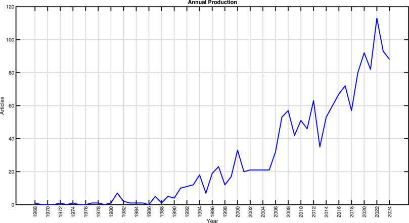
Figure 2. Annual increase of EM papers from 1982 to 2023.

5.1 EM’s bibliometric performance evolution

Traditionally, the number of citations and the average citations per paper have been used to measure the impact of scientific research. However, the varying citation styles across different scientific fields make comparisons using only the number of citations or the impact factor inadequate. Furthermore, citation levels change over time within the same scientific field, and the type of publication also influences the number of citations received; for instance, review articles tend to receive more citations than regular articles. For this reason, the bibliometric community has worked on designing indicators that enable comparisons of scientific impact across different fields. The goal of this section is to determine the impact of scientific production in the EM field over time. To achieve this, we selected four bibliometric impact indicators, normalized by research area, document type, and year of publication. These indicators are as follows: Category Normalized Citation Impact (CNCI), Percentage of Documents in the Top 1%, Documents in the Top 10%, and Average Percentile (AP). In addition to these four indicators, we include the total number of documents and the percentage of documents produced through international collaboration. These six indicators characterize the performance profile of EM research.

To analyze how the performance profile of EM research has evolved, we used these indicators for each year during the period 2000–2023. As outlined in the Methods section, we take advantage of a SOM to visually represent the evolution of the performance profile in two dimensions. Figure 3 shows the SOM neural network representation of the EM’s performance profile evolution. Each year annotated on the maps represents the EM performance profile. Each plot is divided into four regions of varying sizes, determined by agglomerative hierarchical clustering and the silhouette coefficient Rousseeuw (1987). The plots span the years 2000–2023, and the black line represents the temporal evolution of the performance profile in a six-dimensional space. The first indicator, Web of Science Documents, highlights the steady annual increase in publications, as previously shown in Figure 2. The Category Normalized Citation Impact shows a peak in 2003, marked in red, indicating a high number of highly cited publications. A value of 1 in the indicator means that the impact factor is equal to the average impact factor of the field where the articles were published. Therefore, in the years when values above 1 were reached, EM articles received, on average, more citations than the average for the field in which they were published.

Figure 3

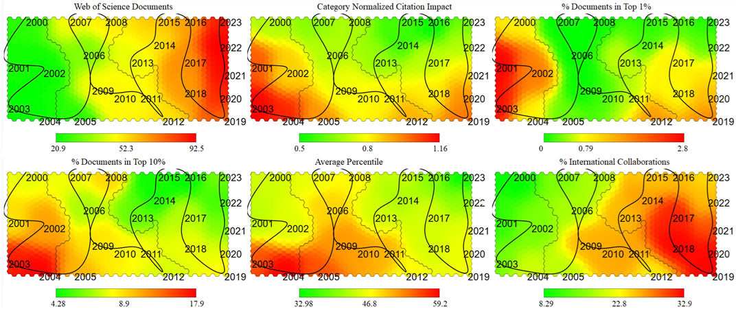
Figure 3. Self-Organizing Map (SOM) visualization of EM’s bibliometric performance profile from 2000 to 2023. Each of the six heatmaps corresponds to a distinct bibliometric indicator that, together, define the annual performance profile. Color intensity reflects the magnitude of each indicator: green denotes lower values, whereas red indicates higher values. The black curve traces the years in chronological order, illustrating the evolutionary path of EM’s performance. This trajectory offers an integrated view of how the six indicators have shifted over time. Overall, the maps indicate a clear trend in the past decade toward greater research output, stronger citation impact, and increased international collaboration.

Looking at the EM inversion field, years with CNCI values exceeding 1 are likely to include publications with exceptionally high individual CNCI scores. For example, in 2001, the average CNCI was 1.47. However, the paper by Rodi and Mackie (2001) achieved a CNCI of 18.511, indicating that it received more than 18 times more citations than the average publication in the same field. Their contributions included the development of a nonlinear conjugate gradient (NLCG) algorithm for 2D magnetotelluric inversion, which significantly improved computational efficiency and reduced memory requirements compared to conventional Gauss-Newton approaches. Similarly, in 2003, Colton et al. (2003) achieved a CNCI of 9.7668, almost ten times the field average. Their study provided a comprehensive survey of the linear sampling method for solving inverse scattering problems involving time-harmonic electromagnetic waves. Their work advanced the understanding of regularization techniques for ill-posed problems and included numerical examples in both 2- and 3-D. In 2012 a notable increase was observed in the CNCNI and the proportion of publications in the Top 1%. That year, the paper by Martin et al. (2012) achieved a CNCI of 18.75, reflecting its substantial influence. The authors addressed computational challenges in large-scale Bayesian inverse problems by introducing a stochastic Newton Markov Chain Monte Carlo (MCMC) method. Their approach leveraged gradient and Hessian information to construct local Gaussian approximations, significantly improving computational efficiency.

Also in 2012, the paper by Egbert and Kelbert (2012) achieved a CNCI of 16.27. Their work established a generalized mathematical framework for computing Jacobians in electromagnetic geophysical inversions, enabling the development of modular inversion codes applicable to diverse active- and passive-source EM methodologies.

In 2019, a paradigm shift occurred with the publication of two machine learning studies: Li et al. (2019) and Puzyrev (2019). Remarkably, these works achieved unprecedented citation impact, with Li et al. (2019) attaining a Category Normalized Citation Impact (CNCI) of 20.75 and Puzyrev (2019) reaching a CNCI of 19.19 -the highest values recorded in the field at the time. These metrics signify that both articles were cited approximately 20 times more frequently than the average publication in their respective research categories, underscoring their exceptional influence and the transformative nature of their contributions.

The next two indicators, Percentage of Documents in the Top 1% and Documents in the Top 10%, follow a similar trend over the years, with 2003 coinciding with the highest value in CNCI. It should be noted that, for these two indicators, the maximum values achieved exceed the expected values (1% and 10%, respectively). In 2003, 2.8% of the articles published in EM were among the top 1% most cited in the field. Similarly, nearly 18% of the publications ranked within the top 10% most cited. Similarly to the previous indicators, the Average Percentile reaches its peak in 2003 and then declines by half in more recent years. An interesting aspect of the Percentage of International Collaborations is its significant increase over time, despite a decline in citation numbers. This indicator reaches its highest point between 2017 and 2019, followed by a slow decrease over the past 5 years.

5.2 Nation’s contribution to EM

As expected, the United States and the People’s Republic of China lead with 23.77% and 29.44% of the total documents, respectively. However, in the last 5 years of the analyzed period (2019–2023), China accounts for 48.3% of the documents, while the United States accounts for 17%. To evaluate each country’s contribution to the domain and their bibliometric performance, we characterized their profiles using the following six bibliometric indicators: Share (the country’s percentage contribution to the domain), National Share (% E−3) (the domain’s share within the country), Category Normalized Citation Impact (CNCI, citations normalized by thematic category, publication year, and document type), % Documents in Top 10% (percentage of documents among the top 10% most cited), Average Percentile, and % Corresponding Author (2008–2024) (percentage of documents with a corresponding author from the country). Each country’s performance profile is represented as a vector of six indicators. Given the challenges of directly comparing multidimensional data, we utilized a SOM neural network to classify and visualize the performance of the countries.

Figure 4 presents the comparisons made by the neural network. In this case, the internal divisions within the figures represent differences in performance profiles. While most countries have unique profiles, the proximity between them indicates similarity. In some cases, countries with highly similar profiles were placed in the same cluster by the neural network. While the United States and China lead in the global share of documents in this field, when this indicator is normalized per country’s total production (as we can see in National Share (%, E−3)), both countries lose their dominance. In contrast, although Singapore and Hong Kong have a lower Share, they exhibit strong performance in the Category Normalized Citation Impact, the % Documents in Top 10% and Average Percentile. The United States also maintains a relatively high performance in these three indicators. Note that in the maps of these three indicators, approximately one-third of the countries are shown in red and orange. These areas represent countries with a higher proportion of documents that perform well in terms of citations. In contrast, countries on the left side of the maps exhibit lower citation performance. Interestingly, some countries located in the low-performance zone, such as Türkiye, Iran, Taiwan, and South Korea, have a high percentage of documents authored by corresponding authors. This suggests that, although their documents may not have high impact, these countries are leading their own investigations. The Average Percentile (AP) indicator complements the impact indicator, as it is less sensitive to outliers than the CNCI. Both are calculated as averages across documents, but documents with an atypically high CNCI receive a percentile of 100 (the highest possible), limiting the variation range of the AP indicator. An example of the differences between these indicators can be seen with France and Australia, which have above-average CNCI values (orange) but average values in the AP. On the other hand, Spain and Germany show the opposite trend, with higher AP values but lower CNCI. This suggests that Australia and Germany have some highly cited documents that raise their CNCI, giving them a better indicator compared to Spain and Germany. However, in the AP, Spain and Germany outperform Australia and France. Additionally, France has low values in % Documents in the Top 10%, indicating that they lack a consolidated group of researchers consistently producing high-performance documents.

Figure 4

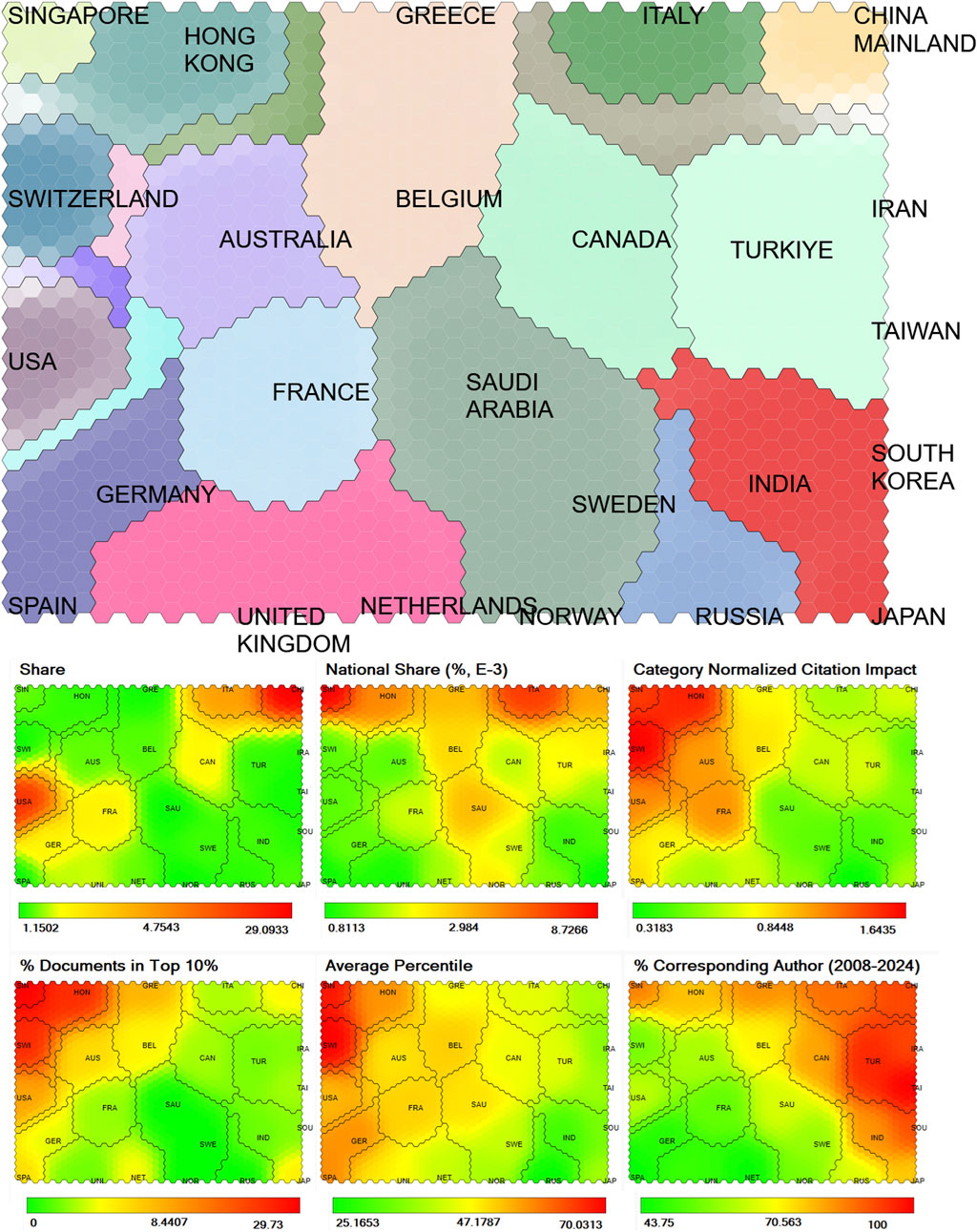
Figure 4. Self-Organizing Map (SOM) clustering of countries based on their multidimensional research performance profiles in EM. The main clustering map (top) groups countries with similar profiles. Countries located in the same or adjacent colored regions (e.g., United States and Switzerland) share comparable performance characteristics, while each colored zone represents a distinct profile type. The six accompanying heatmaps (bottom) display the distribution of individual indicators across the map. As in Figure 3, green indicates lower values and red indicates higher values. A country’s performance can be interpreted by locating it on the clustering map and then examining the corresponding areas in the six heatmaps. For example, countries in the top-left corner (e.g., Singapore, Switzerland) show high citation impact (Category Normalized Citation Impact) and a large share of documents in the top $10\%$, whereas those in the right-side cluster (e.g., India, South Korea, Japan) display different, yet distinctive, strengths.

5.3 EM’s thematic structure

Figure 5 presents an author keyword co-occurrence map, with color indicating the progression of time. Yellow represents more recent keyword co-occurrences, while green corresponds to the oldest keywords in the literature, considering a time span from 2010 to 2023. The color gradient reflects the evolution of keyword co-occurrence over time. The larger nodes represent higher occurrence frequencies. The most prominent co-occurring keywords are Inverse problems, Inverse scattering, and Electromagnetic inverse scattering. It is important to note that certain keywords appear multiple times due to variations such as singular versus plural forms or the inclusion of apostrophes, as in “Maxwell’s equations” and “Maxwell equations.” Despite this redundancy, it is noteworthy that computational methods and ML have recently emerged as impactful approaches in this domain. In the upper right section of the network (Figure 5), the newly introduced keywords can be observed, representing emerging topics in electromagnetics (EM). These topics may be regarded as a new research front within the EM field. Notably, the “deep learning” node, owing to its high connectivity with classical topics, is establishing itself as a central theme within this network.

Figure 5

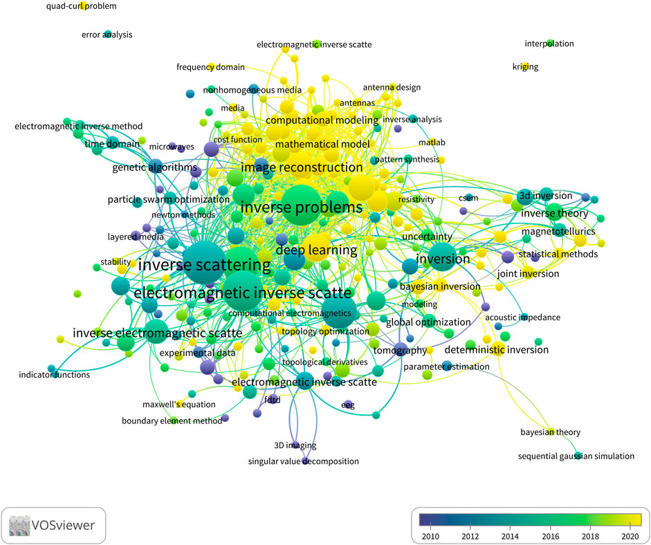
Figure 5. Author keyword co-occurrence network. Node size indicates the frequency of each keyword, edge thickness represents the strength of co-occurrence between keywords, and node color denotes cluster membership. An interactive version of the network is available at https://app.vosviewer.com/AuthorKeyWord.

6 Conclusions

This study provides a comprehensive and integrated analysis of EM modeling by synthesizing a systematic review of deterministic, non-deterministic, and ML-based methodologies with a bibliometric evaluation of the field’s evolution. We examined the theoretical foundations, practical applications, and limitations of each approach, focusing on how they address the intrinsic challenges of the EM inverse problem, such as nonlinearity, ill-posedness, and the need for accurate subsurface reconstructions. Deterministic methods, long considered the cornerstone of EM modeling, offer robust solutions in well-constrained scenarios and are typically characterized by their mathematical rigor and computational efficiency. However, these methods struggle with the uncertainty inherent in complex, heterogeneous subsurface environments, often requiring significant assumptions that limit their applicability in real-world settings. Non-deterministic approaches, including stochastic and probabilistic methods, provide a framework for uncertainty quantification and are better suited for addressing ill-posed problems. These methods offer greater flexibility, accommodating complex geophysical conditions and capturing variability in subsurface structures, but they are hindered by high computational costs and the need for sophisticated sampling strategies.

The advent of ML techniques signifies a major advancement in the field, providing promising solutions to address several limitations inherent in traditional methods. These ML-based approaches exhibit considerable potential in automating data preprocessing, expediting inversion workflows, and improving the accuracy of subsurface reconstructions. However, challenges persist, notably in achieving robust generalization across diverse geophysical environments and the reliance on large, high-quality training datasets. Despite these obstacles, the incorporation of ML techniques into inverse EM modeling represents a transformative development, facilitating more efficient and precise modeling workflows.

In addition to exploring methodological advancements, this study has highlighted the ongoing efforts to bridge the gap between data accuracy and computational power. The increasing complexity of EM models, particularly in three-dimensional and multi-scale scenarios, necessitates substantial computational resources. Recent advancements in high-performance computing (HPC) and parallel processing have enabled the simulation of larger and more intricate models (Castillo-Reyes et al., 2024), addressing some of the computational limitations faced by traditional methods. Furthermore, the push for more accurate data—through improved measurement techniques and instrumentation—remains central to advancing the field. Enhanced data resolution and precision are crucial for producing more accurate subsurface reconstructions and for validating complex models.

Furthermore, by utilizing unsupervised NNs, specifically SOM, this study revealed latent patterns within large-scale datasets that conventional literature review methods may fail to identify. Through the application of SOM techniques, we conducted a comprehensive bibliometric assessment to quantify, interpret, and evaluate the topic of interest. The bibliometric assessment highlights the consistent expansion of EM publications over the past two decades, with a significant surge in influence around 2003, which continues to shape the field today. The period from 2019 to 2021 was marked by an increase in both research output and impact indicators. However, the subsequent decline observed in 2022 and 2023 suggests a potential shift in the field, possibly indicating the emergence of new challenges or research domains that necessitate alternative methodologies and approaches. These trends emphasize the dynamic and evolving nature of the field, characterized by oscillating patterns in research emphasis and impact.

Finally, the insights presented here underscore the need for the continued development of more efficient, adaptable, and interdisciplinary methodologies. Future advancements in inverse EM modeling will depend on addressing the growing demands for improved data accuracy, computational power, and the integration of ML techniques. We hope that this work provides a clear direction for future research, laying the foundation for innovations that can transform the application of inverse EM modeling in subsurface exploration and beyond.

Author contributions

OC: Conceptualization, Formal Analysis, Funding acquisition, Investigation, Methodology, Supervision, Writing – original draft, Writing – review and editing. JJ-A: Data curation, Formal Analysis, Investigation, Visualization, Writing – review and editing. RD: Conceptualization, Investigation, Methodology, Writing – review and editing. UI-V: Investigation, Methodology, Writing – review and editing.

Funding

The author(s) declare that financial support was received for the research and/or publication of this article. The work of OC have received funding from the MCIN/AEI/10.13039/501100011033 (Spain) and from the European Union NextGenerationEU/PRTR under the project GEOTHERPAL-EM_TED2021-131882B-C42 and -C41. OC has also been partially financed by Generalitat de Catalunya (AGAUR) under grant agreement 2021-SGR-00478. JJ-A has received support form DGAPA-UNAM IN310325. UI-V was partially supported by JST SATREPS Japan Grant Number JPMJSA2310; DGAPA-UNAM project numbers: IN111823, IN107720 and CONAHCYT México under Ciencia de Frontera Project Number: 6655. Finally, this work has been partially financed by the Spanish Ministry of Science (MICINN), the Research State Agency (AEI) and European Regional Development Funds (ERDF/FEDER) under grant agreement PID2021-126248OB-I00, MCIN/AEI/10.13039/ 501100011033/FEDER, UE. Authors thanks to Josep Ll. Berral (UPC) and the CROMAI team (UPC) for their support on this research.

Conflict of interest

The authors declare that the research was conducted in the absence of any commercial or financial relationships that could be construed as a potential conflict of interest.

Generative AI statement

The author(s) declare that no Generative AI was used in the creation of this manuscript.

Any alternative text (alt text) provided alongside figures in this article has been generated by Frontiers with the support of artificial intelligence and reasonable efforts have been made to ensure accuracy, including review by the authors wherever possible. If you identify any issues, please contact us.

Publisher’s note

All claims expressed in this article are solely those of the authors and do not necessarily represent those of their affiliated organizations, or those of the publisher, the editors and the reviewers. Any product that may be evaluated in this article, or claim that may be made by its manufacturer, is not guaranteed or endorsed by the publisher.

References

Abubakar, A., Liu, J., Li, M., Habashy, T. M., and MacLennan, K. (2010). “Sensitivity study of multi-sources receivers CSEM data for TI-anisotropy medium using 2.5D forward and inversion algorithm,” in 72nd Annual International Conference and Exhibition (EAGE: Barcelona, Spain). doi:10.3997/2214-4609.201400664

CrossRef Full Text | Google Scholar

Alberts, A., and Bilionis, I. (2024). On the well-posedness of inverse problems under information field theory: application to model-form error detection. arXiv preprint arXiv:2401.14224.

Google Scholar

Amaya, M., Morten, J. P., and Boman, L. (2016). A low-rank approximation for large-scale 3D controlled-source electromagnetic Gauss-Newton inversion. Geophysics 81 (3), E211–E225. doi:10.1190/geo2015-0079.1

CrossRef Full Text | Google Scholar

Arbogast, T., Dawson, C. N., Keenan, P. T., Wheeler, M. F., and Yotov, I. (1998). Enhanced cell-centered finite differences for elliptic equations on general geometry. SIAM. J. Sci. Comput. 19 (2), 404–425. doi:10.1137/S1064827594264545

CrossRef Full Text | Google Scholar

Ardid, A., Dempsey, D., Bertrand, E., Sepulveda, F., Tarits, P., Solon, F., et al. (2021). Bayesian magnetotelluric inversion using methylene blue structural priors for imaging shallow conductors in geothermal fields. Geophysics 86 (3), E171–E183. doi:10.1190/geo2020-0226.1

CrossRef Full Text | Google Scholar

Asif, M. R., Foged, N., Bording, T., Larsen, J. J., and Christiansen, A. V. (2023). DL-RMD: a geophysically constrained electromagnetic resistivity model database (RMD) for deep learning (DL) applications. Earth Syst. Sci. Data 15 (3), 1389–1401. doi:10.5194/essd-15-1389-2023

CrossRef Full Text | Google Scholar

Avdeev, D. B. (2005). Three-dimensional electromagnetic modelling and inversion from theory to application. Surv. Geophys. 26 (6), 767–799. doi:10.1007/s10712-005-1836-x

CrossRef Full Text | Google Scholar

Avdeev, D., and Avdeeva, A. (2009). 3D magnetotelluric inversion using a limited-memory quasi-newton optimization. Geophysics 74 (3), F45–F57. doi:10.1190/1.3114023

CrossRef Full Text | Google Scholar

Avdeev, D. B., Kuvshinov, A. V., Pankratov, O. V., and Newman, G. A. (2002). Three-dimensional induction logging problems, part I: an integral equation solution and model comparisons. Geophysics 67 (2), 413–426. doi:10.1190/1.1468601

CrossRef Full Text | Google Scholar

Ayani, M., MacGregor, L., and Mallick, S. (2020). Inversion of marine controlled source electromagnetic data using a parallel non-dominated sorting genetic algorithm. Geophys. J. Int. 220 (2), 1066–1077. doi:10.1093/gji/ggz501

CrossRef Full Text | Google Scholar

Baumeister, J. (1987). Stable solution of inverse problems. Springer.

Google Scholar

Bian, J., Ruan, D., Wang, Y., Sun, X., and Gu, Z. (2023). Bayesian ensemble machine learning-assisted deterministic and stochastic groundwater dnapl source inversion with a homotopy-based progressive search mechanism. J. Hydrology 624, 129925. doi:10.1016/j.jhydrol.2023.129925

CrossRef Full Text | Google Scholar

Blatter, D., Key, K., Ray, A., Gustafson, C., and Evans, R. (2019). Bayesian joint inversion of controlled source electromagnetic and magnetotelluric data to image freshwater aquifer offshore New Jersey. Geophys. J. Int. 218 (3), 1822–1837. doi:10.1093/gji/ggz253

CrossRef Full Text | Google Scholar

Börner, R.-U. (2010). Numerical modelling in geo-electromagnetics: advances and challenges. Surv. Geophys. 31 (2), 225–245. doi:10.1007/s10712-009-9087-x

CrossRef Full Text | Google Scholar

Brown, V., Hoversten, M., Key, K., and Chen, J. (2012). Resolution of reservoir scale electrical anisotropy from marine CSEM data. Geophysics 77 (2), E147–E158. doi:10.1190/geo2011-0159.1

CrossRef Full Text | Google Scholar

Buland, A., and Kolbjørnsen, O. (2012). Bayesian inversion of CSEM and magnetotelluric data. Geophysics 77 (1), E33–E42. doi:10.1190/geo2010-0298.1

CrossRef Full Text | Google Scholar

Cai, H., Hu, X., Li, J., Endo, M., and Xiong, B. (2017). Parallelized 3D CSEM modeling using edge-based finite element with total field formulation and unstructured mesh. Comput. and Geosciences 99, 125–134. doi:10.1016/j.cageo.2016.11.009

CrossRef Full Text | Google Scholar

Cai, H., Long, Z., Lin, W., Li, J., Lin, P., and Hu, X. (2021). 3D multinary inversion of controlled-source electromagnetic data based on the finite-element method with unstructured mesh. Geophysics 86 (1), E77–E92. doi:10.1190/geo2020-0164.1

CrossRef Full Text | Google Scholar

Campanyà, J., Ledo, J., Queralt, P., Marcuello, A., Liesa, M., and Muñoz, J. A. (2012). New geoelectrical characterisation of a continental collision zone in the west-central pyrenees: constraints from long period and broadband magnetotellurics. Earth Planet. Sci. Lett. 333, 112–121. doi:10.1016/j.epsl.2012.04.018

CrossRef Full Text | Google Scholar

Carazzone, J., Dickens, T., Green, K., Jing, C., Willen, D., Wahrmund, L., et al. (2008). “Inversion study of a large marine CSEM survey,” in SEG International Exposition and Annual Meeting (Vegas, United States: SEG). doi:10.1190/1.3063733

CrossRef Full Text | Google Scholar

Castillo-Reyes, O., de la Puente, J., and Cela, J. M. (2018). PETGEM: a parallel code for 3D CSEM forward modeling using edge finite elements. Comput. and Geosciences 119, 123–136. doi:10.1016/j.cageo.2018.07.005

CrossRef Full Text | Google Scholar

Castillo-Reyes, O., de la Puente, J., García-Castillo, L. E., and Cela, J. M. (2019). Parallel 3D marine controlled-source electromagnetic modeling using high-order tetrahedral nédélec elements. Geophys. J. Int. 219, 39–65. doi:10.1093/gji/ggz285

CrossRef Full Text | Google Scholar

Castillo-Reyes, O., Hu, X., Wang, B., Wang, Y., and Guo, Z. (2023a). Electromagnetic imaging and deep learning for transition to renewable energies: a technology review. Front. Earth Sci. 11, 1159910. doi:10.3389/feart.2023.1159910

CrossRef Full Text | Google Scholar

Castillo-Reyes, O., Rulff, P., Schankee Um, E., and Amor-Martin, A. (2023b). Meshing strategies for 3D geo-electromagnetic modeling in the presence of metallic infrastructure. Comput. Geosci. 27, 1023–1039. doi:10.1007/s10596-023-10247-w

CrossRef Full Text | Google Scholar

Castillo-Reyes, O., Queralt, P., Piñas-Varas, P., Ledo, J., and Rojas, O. (2024). Electromagnetic subsurface imaging in the presence of metallic structures: a review of numerical strategies. Surv. Geophys., 1–35. doi:10.1007/s10712-024-09855-7

CrossRef Full Text | Google Scholar

Chambers, J. E., Kuras, O., Meldrum, P. I., Ogilvy, R. D., and Hollands, J. (2006). Electrical resistivity tomography applied to geologic, hydrogeologic, and engineering investigations at a former waste-disposal site. Geophysics 71 (6), B231–B239. doi:10.1190/1.2360184

CrossRef Full Text | Google Scholar

Chang, P.-Y., Chang, L.-C., Hsu, S.-Y., Tsai, J.-P., and Chen, W.-F. (2017). Estimating the hydrogeological parameters of an unconfined aquifer with the time-lapse resistivity-imaging method during pumping tests: case studies at the Pengtsuo and Dajou sites, Taiwan. J. Appl. Geophys. 144, 134–143. doi:10.1016/j.jappgeo.2017.06.014

CrossRef Full Text | Google Scholar

Chauhan, I., and Dehiya, R. (2024). Two-dimensional controlled source electromagnetic inversion algorithm based on a space domain forward modeling approach. Geophys. Prospect. 72 (8), 3052–3066. doi:10.1111/1365-2478.13575

CrossRef Full Text | Google Scholar

Chopard, B., and Tomassini, M. (2018). An introduction to metaheuristics for optimization. Springer. doi:10.1007/978-3-319-93073-2

CrossRef Full Text | Google Scholar

Colton, D., Haddar, H., and Piana, M. (2003). The linear sampling method in inverse electromagnetic scattering theory. Inverse Probl. 19 (6), S105–S137. doi:10.1088/0266-5611/19/6/057

CrossRef Full Text | Google Scholar

Commer, M., and Newman, G. A. (2008). New advances in three-dimensional controlled-source electromagnetic inversion. Geophys. J. Int. 172, 513–535. doi:10.1111/j.1365-246X.2007.03663.x

CrossRef Full Text | Google Scholar

Constable, S. (2006). Marine electromagnetic methods - a new tool for offshore exploration. Lead. Edge 25 (4), 438–444. doi:10.1190/1.2193225

CrossRef Full Text | Google Scholar

Constable, S. (2010). Ten years of marine CSEM for hydrocarbon exploration. Geophysics 75 (5), 75A67–75A81. doi:10.1190/1.3483451

CrossRef Full Text | Google Scholar

Coppo, N., Darnet, M., Harcouet-Menou, V., Wawrzyniak, P., Manzella, A., Bretaudeau, F., et al. (2016). “Characterization of deep geothermal energy resources in low enthalpy sedimentary basins in Belgium using electro-magnetic methods–CSEM and MT results,” in European Geothermal Congress 2016.

Google Scholar

Daniel, J. W. (1967). The conjugate gradient method for linear and nonlinear operator equations. SIAM J. Numer. Analysis 4 (1), 10–26. doi:10.1137/0704002

CrossRef Full Text | Google Scholar

Davydycheva, S., Druskin, V., and Habashy, T. (2003). An efficient finite-difference scheme for electromagnetic logging in 3D anisotropic inhomogeneous media. Geophysics 68 (5), 1525–1536. doi:10.1190/1.1620626

CrossRef Full Text | Google Scholar

Dehiya, R. (2021). 3D forward modeling of controlled-source electromagnetic data based on the radiation boundary method. Geophysics 86 (2), E143–E155. doi:10.1190/geo2020-0107.1

CrossRef Full Text | Google Scholar

Dehiya, R. (2024). Error propagation and model update analysis in three-dimensional CSEM inversion. Geophys. J. Int. 238 (3), 1807–1824. doi:10.1093/gji/ggae251

CrossRef Full Text | Google Scholar

Dehiya, R., Singh, A., Gupta, P. K., and Israil, M. (2017a). Optimization of computations for adjoint field and jacobian needed in 3D CSEM inversion. J. Appl. Geophys. 136, 444–454. doi:10.1016/j.jappgeo.2016.11.018

CrossRef Full Text | Google Scholar

Dehiya, R., Singh, A., Gupta, P. K., and Israil, M. (2017b). 3-D CSEM data inversion algorithm based on simultaneously active multiple transmitters concept. Geophys. J. Int. 209 (2), 1004–1017. doi:10.1093/gji/ggx062

CrossRef Full Text | Google Scholar

Donthu, N., Kumar, S., Mukherjee, D., Pandey, N., and Lim, W. M. (2021). How to conduct a bibliometric analysis: an overview and guidelines. J. Bus. Res. 133, 285–296. doi:10.1016/j.jbusres.2021.04.070

CrossRef Full Text | Google Scholar

Eck, N. J. V., and Waltman, L. (2010). Software survey: VOSviewer, a computer program for bibliometric mapping. Scientometrics 84, 523–538. doi:10.1007/S11192-009-0146-3/FIGURES/7

PubMed Abstract | CrossRef Full Text | Google Scholar

Egbert, G. D., and Kelbert, A. (2012). Computational recipes for electromagnetic inverse problems. Geophys. J. Int. 189 (1), 251–267. doi:10.1111/j.1365-246X.2011.05347.x

CrossRef Full Text | Google Scholar

Eidesmo, T., Ellingsrud, S., MacGregor, L., Constable, S., Sinha, M., Johansen, S., et al. (2002). Sea bed logging (SBL), a new method for remote and direct identification of hydrocarbon filled layers in deepwater areas. First break 20 (3), 144–152. doi:10.3997/1365-2397.20.3.25008

CrossRef Full Text | Google Scholar

Ernst, O., Nobile, F., Schillings, C., and Sullivan, T. (2020). Uncertainty quantification. Oberwolfach Rep. 16 (1), 695–772. doi:10.4171/owr/2019/12

CrossRef Full Text | Google Scholar

Etgen, J., Gray, S. H., and Zhang, Y. (2009). An overview of depth imaging in exploration geophysics. Geophysics 74 (6), WCA5–WCA17. doi:10.1190/1.3223188

CrossRef Full Text | Google Scholar

Fortunato, S., Bergstrom, C. T., Börner, K., Evans, J. A., Helbing, D., Milojević, S., et al. (2018). Science of science. Science 359, eaao0185. doi:10.1126/science.aao0185

PubMed Abstract | CrossRef Full Text | Google Scholar

Gehrmann, R. A., Schwalenberg, K., Riedel, M., Spence, G. D., Spieß, V., and Dosso, S. E. (2015). Bayesian inversion of marine controlled source electromagnetic data offshore Vancouver Island, Canada. Geophys. J. Int. 204 (1), 21–38. doi:10.1093/gji/ggv437

CrossRef Full Text | Google Scholar

Girard, J.-F., Coppo, N., Rohmer, J., Bourgeois, B., Naudet, V., and Schmidt-Hattenberger, C. (2011). Time-lapse CSEM monitoring of the Ketzin (Germany) CO₂ injection using 2 × MAM configuration. Energy Procedia 4, 3322–3329. doi:10.1016/j.egypro.2011.02.253

CrossRef Full Text | Google Scholar

González, J. R., Sancho-Royo, A., Pelta, D. A., and Cruz, C. (2008). “Nature-inspired cooperative strategies for optimization,” in Encyclopedia of networked and virtual organizations (United Kingdom: IGI Global), 982–989. doi:10.1007/978-3-642-12538-6

CrossRef Full Text | Google Scholar

Grandis, H., Menvielle, M., and Roussignol, M. (1999). Bayesian inversion with Markov chains—I. The magnetotelluric one-dimensional case. Geophys. J. Int. 138 (3), 757–768. doi:10.1046/j.1365-246x.1999.00904.x

CrossRef Full Text | Google Scholar

Grant, M. J., and Booth, A. (2009). A typology of reviews: an analysis of 14 review types and associated methodologies. Health Inf. and Libr. J. 26 (2), 91–108. doi:10.1111/j.1471-1842.2009.00848.x

PubMed Abstract | CrossRef Full Text | Google Scholar

Grayver, A. V., and Bürg, M. (2014). Robust and scalable 3-D geo-electromagnetic modelling approach using the finite element method. Geophys. J. Int. 198 (1), 110–125. doi:10.1093/gji/ggu119

CrossRef Full Text | Google Scholar

Grayver, A. V., Streich, R., and Ritter, O. (2013). Three-dimensional parallel distributed inversion of CSEM data using a direct forward solver. Geophys. J. Int. 193 (3), 1432–1446. doi:10.1093/gji/ggt055

CrossRef Full Text | Google Scholar

Green, B. F., and Hall, J. A. (1984). Quantitative methods for literature reviews. Annu. Rev. Psychol. 35 (1), 37–54. doi:10.1146/annurev.ps.35.020184.000345

PubMed Abstract | CrossRef Full Text | Google Scholar

Gribenko, A., and Zhdanov, M. (2007). Rigorous 3D inversion of marine CSEM data based on the integral equation method. Geophysics 72 (2), WA73–WA84. doi:10.1190/1.2435712

CrossRef Full Text | Google Scholar

Groetsch, C. W., and Groetsch, C. (1993). Inverse problems in the mathematical sciences, volume 52. Springer.

Google Scholar

Gunning, J., Glinsky, M. E., and Hedditch, J. (2010). Resolution and uncertainty in 1D CSEM inversion: a bayesian approach and open-source implementation. Geophysics 75 (6), F151–F171. doi:10.1190/1.3496902

CrossRef Full Text | Google Scholar

Guo, R., Huang, T., Li, M., Zhang, H., and Eldar, Y. C. (2023). Physics-embedded machine learning for electromagnetic data imaging: examining three types of data-driven imaging methods. IEEE Signal Process. Mag. 40 (2), 18–31. doi:10.1109/MSP.2022.3198805

CrossRef Full Text | Google Scholar

Haber, E. (2005). Quasi-Newton methods for large scale electromagnetic inverse problem. Inverse Probl. 21, 305–317. doi:10.1088/0266-5611/21/1/019

CrossRef Full Text | Google Scholar

Haber, E., Ascher, U. M., Aruliah, D. A., and Oldenburg, D. W. (2000). On optimization techniques for solving nonlinear inverse problems. Inverse Probl. 16, 1263–1280. doi:10.1088/0266-5611/16/5/309

CrossRef Full Text | Google Scholar

Han, Y., and Misra, S. (2021). “Chapter 7 - deterministic inversion of galvanic resistivity, induction resistivity, propagation resistivity, and dielectric dispersion logs,” in Multifrequency electromagnetic data interpretation for subsurface characterization. Editors S. Misra, Y. Han, Y. Jin, and P. Tathed (Elsevier), 209–238. doi:10.1016/B978-0-12-821439-8.00006-9

CrossRef Full Text | Google Scholar

Hansen, K., Panzner, M., Shantsev, D., and Mohn, K. (2018). “Comparison of TTI and VTI 3D inversion of CSEM data,” in 80th EAGE Conference and Exhibition 2018 (Copenhagen, Denmark: European Association of Geoscientists and Engineers), 1–5. doi:10.3997/2214-4609.201800752

CrossRef Full Text | Google Scholar

Heagy, L. J., Cockett, R., Kang, S., Rosenkjaer, G. K., and Oldenburg, D. W. (2017). A framework for simulation and inversion in electromagnetics. Comput. and Geosciences 107, 1–19. doi:10.1016/j.cageo.2017.06.018

CrossRef Full Text | Google Scholar

Hermeline, F. (2009). A finite volume method for approximating 3D diffusion operators on general meshes. J. Comput. Phys. 228 (16), 5763–5786. doi:10.1016/j.jcp.2009.05.002

CrossRef Full Text | Google Scholar

Hördt, A., Druskin, V. L., Knizhnerman, L. A., and Strack, K.-M. (1992). Interpretation of 3-D effects in long-offset transient electromagnetic (LOTEM) soundings in the Münsterland area/Germany. Geophysics 57 (9), 1127–1137. doi:10.1190/1.1443327

CrossRef Full Text | Google Scholar

Hördt, A., Dautel, S., Tezkan, B., and Thern, H. (2000). Interpretation of long-offset transient electromagnetic data from the Odenwald area, Germany, using two-dimensional modelling. Geophys. J. Int. 140 (3), 577–586. doi:10.1046/j.1365-246X.2000.00047.x

CrossRef Full Text | Google Scholar

Hu, Y.-D., Wang, X.-H., Zhou, H., Wang, L., and Wang, B.-Z. (2023). A more general electromagnetic inverse scattering method based on physics-informed neural network. IEEE Trans. Geoscience Remote Sens. 61, 1–9. doi:10.1109/TGRS.2023.3301455

CrossRef Full Text | Google Scholar

Jahandari, H., and Farquharson, C. G. (2014). A finite-volume solution to the geophysical electromagnetic forward problem using unstructured grids. Geophysics 79 (6), E287–E302. doi:10.1190/geo2013-0312.1

CrossRef Full Text | Google Scholar

Jahandari, H., Ansari, S., and Farquharson, C. G. (2017). Comparison between staggered grid finite-volume and edge-based finite–element modelling of geophysical electromagnetic data on unstructured grids. J. Appl. Geophys. 138, 185–197. doi:10.1016/j.jappgeo.2017.01.016

CrossRef Full Text | Google Scholar

Jaysaval, P., Datta, D., Sen, M. K., Arnulf, A. F., Denel, B., and Williamson, P. (2019). “2.5 D controlled-source electromagnetic inversion using very fast simulated annealing algorithm,” in SEG International Exposition and Annual Meeting (Denver, United States: SEG). doi:10.1190/segam2019-3211567.1

CrossRef Full Text | Google Scholar

Jiménez-Andrade, J.-L. (2023). “Métodos y Aplicaciones de la Red Neuronal SOM para el Análisis Temporal de Datos Multidimensionales,”. Ph.D. thesis. CDMX, México: Infotec, Centro de Investigación e Innovación en tecnologías de la Información y Comunicación.

Google Scholar

Jiménez-Andrade, J.-L., Villaseñor-García, E.-A., and Carrillo-Calvet, H.-A. (2020). LabSOM (self-organizing maps laboratory).

Google Scholar

Jin, J.-M. (2015). The finite element method in electromagnetics. John Wiley and Sons.

Google Scholar

Jing, C., Green, K., and Willen, D. (2008). “CSEM inversion: impact of anisotropy, data coverage, and initial models,” in SEG Technical Program Expanded Abstracts 2008 (Vegas, United States: Society of Exploration Geophysicists), 604–608. doi:10.1190/1.3063724

CrossRef Full Text | Google Scholar

Key, K. (2016). MARE2DEM: a 2-D inversion code for controlled-source electromagnetic and magnetotelluric data. Geophys. J. Int. 207, 571–588. doi:10.1093/gji/ggw290

CrossRef Full Text | Google Scholar

Key, K., and Ovall, J. (2011). A parallel goal-oriented adaptive finite element method for 2.5-D electromagnetic modelling. Geophys. J. Int. 186 (1), 137–154. doi:10.1111/j.1365-246X.2011.05025.x

CrossRef Full Text | Google Scholar

Kho, J. H., Meju, M. A., Miller, R. V., and Saleh, A. S. (2024). Deep structural controls on the distribution of carbonate reservoirs and overburden heterogeneity in central Luconia province, offshore Borneo revealed by 3D anisotropic inversion of regional controlled-source electromagnetic and magnetotelluric profile data. Geophysics 89 (1), B17–B30.

CrossRef Full Text | Google Scholar

Kim, Y., and Nakata, N. (2018). Geophysical inversion versus machine learning in inverse problems. Lead. Edge 37 (12), 894–901. doi:10.1190/tle37120894.1

CrossRef Full Text | Google Scholar

Kohonen, T. (1981). Automatic formation of topological maps of patterns in a self-organizing system. Berlin-Heildelberg, Germany: Springer.

Google Scholar

Kohonen, T. (1982). Self-organized formation of topologically correct feature maps. Biol. Cybern. 43, 59–69. doi:10.1007/BF00337288

CrossRef Full Text | Google Scholar

Kohonen, T. (2001). Self-organizing maps. 3rd edn. Berlin-Heildelberg, Germany: Springer.

Google Scholar

Kohonen, T. (2013). Essentials of the self-organizing map. Neural Netw. 37, 52–65. doi:10.1016/j.neunet.2012.09.018

PubMed Abstract | CrossRef Full Text | Google Scholar

Laloy, E., Linde, N., Ruffino, C., Hérault, R., Gasso, G., and Jacques, D. (2019). Gradient-based deterministic inversion of geophysical data with generative adversarial networks: is it feasible? Comput. and Geosciences 133, 104333. doi:10.1016/j.cageo.2019.104333

CrossRef Full Text | Google Scholar

Ledo, J., Queralt, P., Martí, A., and Jones, A. G. (2002). Two-dimensional interpretation of three-dimensional magnetotelluric data: an example of limitations and resolution. Geophys. J. Int. 150 (1), 127–139. doi:10.1046/j.1365-246X.2002.01705.x

CrossRef Full Text | Google Scholar

Li, G., Li, Y., Han, B., and Liu, Z. (2018). Application of the perfectly matched layer in 3-D marine controlled-source electromagnetic modelling. Geophys. J. Int. 212 (1), 333–344. doi:10.1093/gji/ggx382

CrossRef Full Text | Google Scholar

Li, L., Wang, L. G., Teixeira, F. L., Liu, C., Nehorai, A., and Cui, T. J. (2019). DeepNIS: deep neural network for nonlinear electromagnetic inverse scattering. IEEE Trans. Antennas Propag. 67 (3), 1819–1825. doi:10.1109/TAP.2018.2885437

CrossRef Full Text | Google Scholar

Liang, H., Gao, R., Yin, C., Su, Y., He, Z., and Liu, Y. (2024). Physics-driven deep-learning for marine CSEM data inversion. J. Appl. Geophys. 229, 105474. doi:10.1016/j.jappgeo.2024.105474

CrossRef Full Text | Google Scholar

Liesen, J., and Strakos, Z. (2013). Krylov subspace methods: principles and analysis. United Kingdom: Numerical Mathematics and Scie.

Google Scholar

Liu, W., Xi, Z., Wang, H., and Zhang, R. (2021). Two-dimensional deep learning inversion of magnetotelluric sounding data. J. Geophys. Eng. 18 (5), 627–641. doi:10.1093/jge/gxab040

CrossRef Full Text | Google Scholar

Liu, H., Fan, Y., Ding, F., Du, L., Zhaoa, J., Sun, C., et al. (2024). Physics-informed deep model for fast time—domain electromagnetic simulation and inversion. IEEE Trans. Antennas Propag. 72 (10), 7807–7820. doi:10.1109/TAP.2024.3433389

CrossRef Full Text | Google Scholar

Ma, J., Deng, Y., Li, X., Guo, R., Zhou, H., and Li, M. (2024). Recent advances in machine learning-enhanced joint inversion of seismic and electromagnetic data. Surv. Geophys. 46, 197–225. doi:10.1007/s10712-024-09867-3

CrossRef Full Text | Google Scholar

Mackie, R. L., Smith, J. T., and Madden, T. R. (1994). Three-dimensional electromagnetic modeling using finite difference equations: the magnetotelluric example. Radio Sci. 29 (4), 923–935. doi:10.1029/94RS00326

CrossRef Full Text | Google Scholar

Malovichko, M., Tarasov, A., Yavich, N., and Zhdanov, M. (2019). Mineral exploration with 3-D controlled-source electromagnetic method: a synthetic study of Sukhoi log gold deposit. Geophys. J. Int. 219 (3), 1698–1716. doi:10.1093/gji/ggz390

CrossRef Full Text | Google Scholar

Martin, J., Wilcox, L. C., Burstedde, C., and Ghattas, O. (2012). A stochastic newton mcmc method for large-scale statistical inverse problems with application to seismic inversion. SIAM J. Sci. Comput. 34 (3), A1460–A1487. doi:10.1137/110845598

CrossRef Full Text | Google Scholar

Meju, M. A., Mackie, R. L., Miorelli, F., Saleh, A. S., and Miller, R. V. (2019). Structurally tailored 3D anisotropic controlled-source electromagnetic resistivity inversion with cross-gradient criterion and simultaneous model calibration. Geophysics 84 (6), E387–E402. doi:10.1190/geo2018-0639.1

CrossRef Full Text | Google Scholar

Mitsuhata, Y., Uchida, T., and Amano, H. (2002). 2.5-D inversion of frequency-domain electromagnetic data generated by a grounded-wire source. Geophysics 67 (6), 1753–1768. doi:10.1190/1.1527076

CrossRef Full Text | Google Scholar

Mittet, R., and Avdeeva, A. (2024). Gauss-newton inversion with node-based basis functions: application to imaging of seabed minerals in an area with rough bathymetry. Geophysics 89 (1), E13–E29. doi:10.1190/geo2022-0763.1

CrossRef Full Text | Google Scholar

Mittet, R., and Morten, J. P. (2012). Detection and imaging sensitivity of the marine CSEM method. Geophysics 77 (6), E411–E425. doi:10.1190/geo2012-0016.1

CrossRef Full Text | Google Scholar

Moed, H. F. (2002). The impact-factors debate: the ISI’s uses and limits. Nature 415, 731–732. doi:10.1038/415731a

PubMed Abstract | CrossRef Full Text | Google Scholar

Moed, H. F. (2017). A critical comparative analysis of five world university rankings. Scientometrics 110, 967–990. doi:10.1007/s11192-016-2212-y

CrossRef Full Text | Google Scholar

Mohamad, S. A., Lorenz, L., Hoong, L. T., Wei, T. K., Chandola, S. K., Saadah, N., et al. (2010). “A practical example why anisotropy matters-A CSEM case study from South East Asia,” in 80th Annual International Meeting (Denver, United States: SEG), 696–700. doi:10.1190/1.3513878

CrossRef Full Text | Google Scholar

Newman, M. E. J. (2001). The structure of scientific collaboration networks. Proc. Natl. Acad. Sci. U. S. A. 92, 404–409. doi:10.1073/pnas.98.2.404

PubMed Abstract | CrossRef Full Text | Google Scholar

Newman, G. A. (2014). A review of high-performance computational strategies for modeling and imaging of electromagnetic induction data. Surv. Geophys. 35 (1), 85–100. doi:10.1007/s10712-013-9260-0

CrossRef Full Text | Google Scholar

Newman, G., and Alumbaugh, D. (1997). Three-dimensional massively parallel electromagnetic inversion—I. Theory. Geophys. J. Int. 128 (2), 345–354. doi:10.1111/j.1365-246X.1997.tb01559.x

CrossRef Full Text | Google Scholar

Newman, G. A., and Alumbaugh, D. L. (2002). Three-dimensional induction logging problems, Part 2: a finite-difference solution. Geophysics 67 (2), 484–491. doi:10.1190/1.1468608

CrossRef Full Text | Google Scholar

Newman, G. A., and Boggs, P. T. (2004). Solution accelerators for large-scale three-dimensional electromagnetic inverse problems. Inverse Probl. 20, S151–S170. doi:10.1088/0266-5611/20/6/S10

CrossRef Full Text | Google Scholar

Newman, G. A., and Hoversten, G. M. (2000). Solution strategies for two-and three-dimensional electromagnetic inverse problems. Inverse probl. 16 (5), 1357–1375. doi:10.1088/0266-5611/16/5/314

CrossRef Full Text | Google Scholar

Newman, G. A., Commer, M., and Carazzone, J. J. (2010). Imaging CSEM data in the presence of electrical anisotropy. Geophysics 75 (2), F51–F61. doi:10.1190/1.3295883

CrossRef Full Text | Google Scholar

Orange, A., Key, K., and Constable, S. (2009). The feasibility of reservoir monitoring using time-lapse marine CSEM. Geophysics 74 (2), F21–F29. doi:10.1190/1.3059600

CrossRef Full Text | Google Scholar

O’Sullivan, F. (1986). A statistical perspective on ill-posed inverse problems. Stat. Sci. 1, 502–518. doi:10.1214/ss/1177013525

CrossRef Full Text | Google Scholar

Paré, G., and Kitsiou, S. (2017). “Methods for literature reviews,” in Handbook of eHealth evaluation: an evidence-based approach (Canada: University of Victoria).

Google Scholar

Park, J., Bjørnarå, T. I., Westerdahl, H., and Gonzalez, E. (2008). “On boundary conditions for CSEM finite element modeling, I,” in COMSOL Multiphysics conference (Germany: Hanover).

Google Scholar

Penz, S., Duchêne, B., and Mohammad-Djafari, A. (2018). Variational bayesian inversion of synthetic 3D controlled-source electromagnetic geophysical data. Geophysics 83 (1), E25–E36. doi:10.1190/geo2016-0682.1

CrossRef Full Text | Google Scholar

Piao, S., Gu, H., Qin, A. W. P., and Qin, P. (2024). A domain-adaptive physics-informed neural network for inverse problems of Maxwell’s equations in heterogeneous media. IEEE Antennas Wirel. Propag. Lett. 23 (10), 2905–2909. doi:10.1109/LAWP.2024.3413851

CrossRef Full Text | Google Scholar

Piña-Varas, P., Ledo, J., Queralt, P., Marcuello, A., Bellmunt, F., Ogaya, X., et al. (2015). Vertical collapse origin of Las Cañadas caldera (Tenerife, Canary Islands) revealed by 3-D magnetotelluric inversion. Geophys. Res. Lett. 42 (6), 1710–1716. doi:10.1002/2015GL063042

CrossRef Full Text | Google Scholar

Plessix, R.-E., Darnet, M., and Mulder, W. (2007). An approach for 3D multisource, multifrequency CSEM modeling. Geophysics 72 (5), SM177–SM184. doi:10.1190/1.2744234

CrossRef Full Text | Google Scholar

Puzyrev, V. (2019). Deep learning electromagnetic inversion with convolutional neural networks. Geophys. J. Int. 218 (2), 817–832. doi:10.1093/gji/ggz204

CrossRef Full Text | Google Scholar

Puzyrev, V., and Swidinsky, A. (2021). Inversion of 1D frequency- and time-domain electromagnetic data with convolutional neural networks. Comput. Ggeosciences 149, 104681. doi:10.1016/j.cageo.2020.104681

CrossRef Full Text | Google Scholar

Queralt, P., Jones, A. G., and Ledo, J. (2007). Electromagnetic imaging of a complex ore body: 3D forward modeling, sensitivity tests, and down-mine measurements. Geophysics 72 (2), F85–F95. doi:10.1190/1.2437105

CrossRef Full Text | Google Scholar

Radicchi, F., Fortunato, S., and Vespignani, A. (2012). Citation networks, understanding complex systems, 233–257. doi:10.1007/978-3-642-23068-4_7

CrossRef Full Text | Google Scholar

Raiche, A. (1974). An integral equation approach to three-dimensional modelling. Geophys. J. Int. 36 (2), 363–376. doi:10.1111/j.1365-246X.1974.tb03645.x

CrossRef Full Text | Google Scholar

Ramananjaona, C., and MacGregor, L. (2010). 2.5 D inversion of CSEM data in a vertically anisotropic earth. J. Phys. Conf. Ser. 255, 012004. doi:10.1088/1742-6596/255/1/012004

CrossRef Full Text | Google Scholar

Ray, A., and Key, K. (2012). Bayesian inversion of marine CSEM data with a trans-dimensional self parametrizing algorithm. Geophys. J. Int. 191 (3), 1135–1151. doi:10.1111/j.1365-246X.2012.05677.x

CrossRef Full Text | Google Scholar

Ray, A., Alumbaugh, D. L., Hoversten, G. M., and Key, K. (2013). Robust and accelerated Bayesian inversion of marine controlled-source electromagnetic data using parallel tempering. Geophysics 78 (6), E271–E280. doi:10.1190/geo2013-0128.1

CrossRef Full Text | Google Scholar

Ray, A., Key, K., Bodin, T., Myer, D., and Constable, S. (2014). Bayesian inversion of marine CSEM data from the scarborough gas field using a transdimensional 2-D parametrization. Geophys. J. Int. 199 (3), 1847–1860. doi:10.1093/gji/ggu370

CrossRef Full Text | Google Scholar

Ren, Z., and Kalscheuer, T. (2020). Uncertainty and resolution analysis of 2D and 3D inversion models computed from geophysical electromagnetic data. Surv. Geophys. 41 (1), 47–112. doi:10.1007/s10712-019-09567-3

CrossRef Full Text | Google Scholar

Rivera-Rios, A. M., Zhou, B., Heinson, G., and Krieger, L. (2019). Multi-order vector finite element modeling of 3D magnetotelluric data including complex geometry and anisotropy. Earth, Planets Space 71 (1), 92–25. doi:10.1186/s40623-019-1071-1

CrossRef Full Text | Google Scholar

Rodi, W., and Mackie, R. L. (2001). Nonlinear conjugate gradients algorithm for 2-D magnetotelluric inversion. Geophysics 66 (1), 174–187. doi:10.1190/1.1444893

CrossRef Full Text | Google Scholar

Rosas-Carbajal, M., Linde, N., Kalscheuer, T., and Vrugt, J. A. (2013). Two-dimensional probabilistic inversion of plane-wave electromagnetic data: methodology, model constraints and joint inversion with electrical resistivity data. United States: Geophys. J. Int. 196 (3), 1508–1524. doi:10.1093/gji/ggt482

CrossRef Full Text | Google Scholar

Rosenthal, R., and DiMatteo, M. R. (2001). Meta-analysis: recent developments in quantitative methods for literature reviews. Annu. Rev. Psychol. 52 (1), 59–82. doi:10.1146/annurev.psych.52.1.59

PubMed Abstract | CrossRef Full Text | Google Scholar

Rousseeuw, P. J. (1987). Silhouettes: a graphical aid to the interpretation and validation of cluster analysis. J. Comput. Appl. Math. 20, 53–65. doi:10.1016/0377-0427(87)90125-7

CrossRef Full Text | Google Scholar

Ruder, S. (2016). An overview of gradient descent optimization algorithms. arXiv preprint arXiv:1609.04747.

Google Scholar

Ruiz-Sánchez, R., Arencibia-Jorge, R., na, J. T., Jiménez-Andrade, J. L., and Carrillo-Calvet, H. (2024). Exploring research on ecotechnology through artificial intelligence and bibliometric maps. Environ. Sci. Ecotechnology 21, 100386. doi:10.1016/j.ese.2023.100386

CrossRef Full Text | Google Scholar

Russell, B. (2019). Machine learning and geophysical inversion - a numerical study. Lead. Edge 38 (7), 512–519. doi:10.1190/tle38070512.1

CrossRef Full Text | Google Scholar

Sagar, M., Ouassal, H., Omi, A., Wisniewska, A., Jalajamony, H., Fernandez, R., et al. (2021). Application of machine learning in electromagnetics: mini-review. Electronics 10, 2752. doi:10.3390/electronics10222752

CrossRef Full Text | Google Scholar

Sarkar, T., Weiner, D., and Jain, V. (1981). Some mathematical considerations in dealing with the inverse problem. IEEE Trans. antennas Propag. 29 (2), 373–379. doi:10.1109/TAP.1981.1142573

CrossRef Full Text | Google Scholar

Schuster, G. T., Chen, Y., and Feng, S. (2024). Review of physics-informed machine-learning inversion of geophysical data. Geophysics 89 (6), T337–T356. doi:10.1190/geo2023-0615.1

CrossRef Full Text | Google Scholar

Seillé, H., and Visser, G. (2020). Bayesian inversion of magnetotelluric data considering dimensionality discrepancies. Geophys. J. Int. 223 (3), 1565–1583. doi:10.1093/gji/ggaa391

CrossRef Full Text | Google Scholar

Shahriari, M., Hazra, A., Pardo, D., and Sobieczky, F. (2020a). A deep neural network as surrogate model for forward simulation of borehole resistivity measurements. Procedia Manuf. 42, 235–238. doi:10.1016/j.promfg.2020.02.075

CrossRef Full Text | Google Scholar

Shahriari, M., Pardo, D., Picón, A., Galdran, A., Del Ser, J., and Torres-Verdín, C. (2020b). A deep learning approach to the inversion of borehole resistivity measurements. Comput. and Geosciences 24, 971–994. doi:10.1007/s10596-019-09859-y

CrossRef Full Text | Google Scholar

Shahriari, M., Hazra, A., and Pardo, D. (2022). A deep learning approach to design a borehole instrument for geosteering. Geophysics 87, D83–D90. doi:10.1190/geo2021-0240.1

CrossRef Full Text | Google Scholar

Sheard, S., Ritchie, T., Christopherson, K., and Brand, E. (2005). Mining, environmental, petroleum, and engineering industry applications of electromagnetic techniques in geophysics. Surv. Geophys 26, 653–669. doi:10.1007/s10712-005-1760-0

CrossRef Full Text | Google Scholar

Siripunvaraporn, W., Egbert, G., Lenbury, Y., and Uyeshima, M. (2005). Three-dimensional magnetotelluric inversion: data-space method. Phys. Earth Planet. interiors 150 (1-3), 3–14. doi:10.1016/j.pepi.2004.08.023

CrossRef Full Text | Google Scholar

Spitzer, K. (2022). “Electromagnetic modeling using adaptive grids - a reflection on the term geometry,” in 25th EM Induction Workshop (Turkey: International Association of Geomagnetism and Aeronomy), 1–5.

Google Scholar

Spitzer, K. (2024). Electromagnetic modeling using adaptive grids-error estimation and geometry representation. Surv. Geophys. 45 (1), 277–314. doi:10.1007/s10712-023-09794-9

CrossRef Full Text | Google Scholar

Srnka, L. J., Carazzone, J. J., Ephron, M. S., and Eriksen, E. A. (2006). Remote reservoir resistivity mapping. Lead. Edge 25 (8), 972–975. doi:10.1190/1.2335169

CrossRef Full Text | Google Scholar

Stratton, J. A. (2007). Electromagnetic theory, volume 33. John Wiley and Sons.

Google Scholar

Sun, Z., Sandoval, L., Crystal-Ornelas, R., Mousavi, S. M., Wang, J., Lin, C., et al. (2022). A review of Earth artificial intelligence. Comput. Geosci. 159, 105034. doi:10.1016/j.cageo.2022.105034

CrossRef Full Text | Google Scholar

Tarantola, A. (2005). Inverse problem theory and methods for model parameter estimation. United States: SIAM.

Google Scholar

Tarantola, A., and Valette, B. (1982). Inverse problems = quest for information. J. Geophys. 50 (1), 159–170.

Google Scholar

Tikhonov, A. N., and Arsenin, V. Y. (1977). Solutions of Ill-posed problems. Washington, D.C., USA: W. H.Winston and Sons.

Google Scholar

Um, E. S., Commer, M., and Newman, G. A. (2013). Efficient pre-conditioned iterative solution strategies for the electromagnetic diffusion in the Earth: finite-element frequency-domain approach. Geophys. J. Int. 193, 1460–1473. doi:10.1093/gji/ggt071

CrossRef Full Text | Google Scholar

Unsworth, M., and Oldenburg, D. (1995). Subspace inversion of electromagnetic data: application to mid-ocean-ridge exploration. Geophys. J. Int. 123 (1), 161–168. doi:10.1111/j.1365-246X.1995.tb06668.x

CrossRef Full Text | Google Scholar

van Eck, N. J., and Waltman, L. (2014). Visualizing bibliometric networks, measuring scholarly impact. Cham: Springer. doi:10.1007/978-3-319-10377-8_13

CrossRef Full Text | Google Scholar

Vilamajó, E., Queralt, P., Ledo, J., and Marcuello, A. (2013). Feasibility of monitoring the Hontomín (Burgos, Spain) CO₂ storage site using a deep EM source. Surv. Geophys. 34 (4), 441–461. doi:10.1007/s10712-013-9238-y

CrossRef Full Text | Google Scholar

Villaseñor, E. A., Arencibia-Jorge, R., and Carrillo-Calvet, H. (2017). Multiparametric characterization of scientometric performance profiles assisted by neural networks: a study of Mexican higher education institutions. Scientometrics 110, 77–104. doi:10.1007/s11192-016-2166-0

CrossRef Full Text | Google Scholar

Wagner, F. M., and Uhlemann, S. (2021). An overview of multimethod imaging approaches in environmental geophysics. Adv. Geophys. 62, 1–72. doi:10.1016/bs.agph.2021.06.001

CrossRef Full Text | Google Scholar

Wang, F., Morten, J. P., and Spitzer, K. (2018). Anisotropic three-dimensional inversion of CSEM data using finite-element techniques on unstructured grids. Geophys. J. Int. 213 (2), 1056–1072. doi:10.1093/gji/ggy029

CrossRef Full Text | Google Scholar

Wang, B., Liu, J., Hu, X., Liu, J., Guo, Z., and Xiao, J. (2021). Geophysical electromagnetic modeling and evaluation: a review. J. Appl. Geophys. 194, 104438. doi:10.1016/j.jappgeo.2021.104438

CrossRef Full Text | Google Scholar

Wannamaker, P. E. (1991). Advances in three-dimensional magnetotelluric modeling using integral equations. Geophysics 56 (11), 1716–1728. doi:10.1190/1.1442984

CrossRef Full Text | Google Scholar

Wannamaker, P. E., Hohmann, G. W., and SanFilipo, W. A. (1984). Electromagnetic modeling of three-dimensional bodies in layered earths using integral equations. Geophysics 49 (1), 60–74. doi:10.1190/1.1441562

CrossRef Full Text | Google Scholar

Werthmüller, D., Rochlitz, R., Castillo-Reyes, O., and Heagy, L. (2021). Towards an open-source landscape for 3-D CSEM modelling. Geophys. J. Int. 227 (1), 644–659. doi:10.1093/gji/ggab238

CrossRef Full Text | Google Scholar

Xiang, E., Guo, R., Dosso, S. E., Liu, J., Dong, H., and Ren, Z. (2018). Efficient hierarchical trans-dimensional bayesian inversion of magnetotelluric data. Geophys. J. Int. 213 (3), 1751–1767. doi:10.1093/gji/ggy071

CrossRef Full Text | Google Scholar

Xiong, Z., and Tripp, A. C. (1997). 3-D electromagnetic modeling for near-surface targets using integral equations. Geophysics 62 (4), 1045–1346. doi:10.1190/1.1444210

CrossRef Full Text | Google Scholar

Xue, G., Li, H., He, Y., Xue, J., and Wu, X. (2020). Development of the inversion method for transient electromagnetic data. IEEE Access 8, 146172–146181. doi:10.1109/ACCESS.2020.3013626

CrossRef Full Text | Google Scholar

Yang, D., and Oldenburg, D. W. (2012). Three-dimensional inversion of airborne time-domain electromagnetic data with applications to a porphyry deposit. Geophysics 77 (2), B23–B34. doi:10.1190/geo2011-0194.1

CrossRef Full Text | Google Scholar

Yao, H., Ren, Z., Tang, J., Guo, R., and Yan, J. (2023). Trans-dimensional bayesian joint inversion of magnetotelluric and geomagnetic depth sounding responses to constrain mantle electrical discontinuities. Geophys. J. Int. 233 (3), 1821–1846. doi:10.1093/gji/ggad029

CrossRef Full Text | Google Scholar

Yoon, D., Zhdanov, M. S., Mattsson, J., Cai, H., and Gribenko, A. (2016). A hybrid finite-difference and integral-equation method for modeling and inversion of marine controlled-source electromagnetic data. Geophysics 81 (5), E323–E336. doi:10.1190/geo2015-0513.1

CrossRef Full Text | Google Scholar

Zhang, G., Zhang, G.-B., Chen, C.-c., Chang, P.-Y., Wang, T.-P., Yen, H.-Y., et al. (2016). Imaging rainfall infiltration processes with the time-lapse electrical resistivity imaging method. Pure Appl. Geophys. 173 (6), 2227–2239. doi:10.1007/s00024-016-1251-x

CrossRef Full Text | Google Scholar

Zhang, P., Deng, M., Jing, J., and Chen, K. (2020). Marine controlled-source electromagnetic method data de-noising based on compressive sensing. J. Appl. Geophys. 177, 104011. doi:10.1016/j.jappgeo.2020.104011

CrossRef Full Text | Google Scholar

Zhang, J.-B., Yu, D.-M., and Pan, X.-M. (2022a). “Physics-informed neural networks for the solution of electromagnetic scattering by integral equations,” in 2022 International Applied Computational Electromagnetics Society Symposium (ACES-China), 1–2. doi:10.1109/ACES-China56081.2022.10065316

CrossRef Full Text | Google Scholar

Zhang, Y., Xu, Y., Yang, B., Mooney, W. D., and Wang, F. (2022b). Geophysical inversions on unstructured meshes using non-gradient based regularization. Geophys. J. Int. 230 (3), 1864–1877. doi:10.1093/gji/ggac155

CrossRef Full Text | Google Scholar

Zhdanov, M. S. (2009). Geophysical electromagnetic theory and methods, volume 43. Elsevier. doi:10.1016/C2014-0-02307-6

CrossRef Full Text | Google Scholar

Zhdanov, M. S. (2010). Electromagnetic geophysics: notes from the past and the road ahead. Geophysics 75 (5), 75A49–75A66. doi:10.1190/1.3483901

CrossRef Full Text | Google Scholar