Abstract
The excavation of high-speed subgrade has formed a large number of subgrade landslides, which have always been a potential threat to highway traffic, and the stability of landslides has an important impact on ensuring the normal operation of highways and traffic safety. In this paper, the on-site engineering geological investigation of a high-speed subgrade landslide is carried out, and the ring shear test is carried out by taking soil samples from slip zone, and the evolution relationship between the friction angle and cohesion in slip zone soil with shear displacement is analyzed by using the Moore-Coulomb theory, and the dynamic evolution law of the shear strength of slip zone soil is revealed. Combined with the typical residual thrust model and the finite element numerical model, the deformation failure mechanism and dynamic stability of the landslide were systematically analyzed. The following conclusions were drawn: The landslide slid again under the inducement of rainfall and gravity, and the overall performance was collapse-slip failure. The friction angle in slip zone soil shows the attenuation trend of the logistic model, and the cohesion shows the attenuation trend of the power function model. With the continuous deformation of landslide, the deformation displacement of landslide gradually showed an increasing trend, and the deformation of the slip zone gradually penetrated from the leading edge and the trailing edge, and the simulation results were basically consistent with the results of the landslide field investigation. With the increase of landslide displacement, the stability of landslide gradually decreases from the peak stability, and finally maintains the residual stability, which is between 1.07 and 1.08. Monitoring and early warning measures should be carried out at any time in the later stage. The landslide stability evaluation has an important safety early warning effect on the normal operation and traffic safety of the expressway.
1 Introduction
With the rapid development of China’s transportation planning, more and more highways have been built. Due to the continuous excavation of subgrade in the mountainous area, a large number of subgrade landslides have been formed, which threaten the safety and operation of the highway at all times (Li and Xie, 2013). Therefore, the stability of subgrade landslides has always attracted much attention (Sarkar et al., 2021). Under the influence of continuous rainfall in mountainous areas, the strength of slip zone in landslide is constantly weakening, which leads to the gradual decline of the stability of the landslide, and the strength of the slip zone affects the stability of the landslide at all times (Liu and Yang, 2011; Chen et al., 2016). The cracks formed by the dry-wet cycle will further reduce the strength of the landslide slide zone (Yang et al., 2024a; Yang et al., 2024b). Therefore, it is of great practical significance to study the stability of subgrade landslide from the perspective of the strength of slip zone soil.
In terms of the strength of slip zone soil, the research mainly focuses on two aspects. On the one hand, it is mainly the influencing factors of the shear mechanical properties of slip zone, including the influence of moisture content (Thaw et al., 2025; Nian et al., 2013), shear rate and over-consolidation ratio (Li and Yang, 2018) on the strength of slip zone. On the other hand, it is mainly the study of strain softening characteristics (Hua et al., 2025; Liu and Chen, 2015) and peak residual strength (Wang et al., 2020; Chen and Liu, 2014) of slip zone soil, that is, the strength of slip zone soil needs to go through five processes during the shearing process: pore shearing, elastic deformation, plastic hardening, strain softening and residual strength. In addition, some scholars have established a shear constitutive model based on statistical damage theory to quantitatively describe the strain softening relationship of the strength of slip zone soil (Zou et al., 2024; Luo et al., 2022), and proved that the proposed constitutive model based on Wei-bull function distribution has the best fitting effect. The above studies only study the variation law of the strength of slip zone soil, but do not deeply analyze the essential characteristics of the strength of slip zone soil. In fact, the strength of slip zone soil is the result of cohesion and friction between the soil particles (Geng et al., 2023; Wang et al., 2024).
In terms of landslide stability, it is mainly divided into two aspects: limit equilibrium and finite element analysis. The calculation method of limit equilibrium method is simple and convenient, and has been widely used in practical engineering calculations. At present, the calculation of landslide stability is mainly realized by the improved residual thrust method (Zou et al., 2020; Yan et al., 2022; Zou et al., 2023a; Zou et al., 2023b), the improved slice-division method (Su et al., 2022; Wu et al., 2019) and the improved vector sum method (Yan et al., 2024). In contrast, the finite element method is more accurate, but it is difficult to be widely used. At present, the finite element numerical simulation combined with the strength reduction method is used to accurately calculate the stability of the landslide (Chen et al., 2019; Yu, 2020). It can be seen that the calculation of landslide stability has been relatively mature, which can be said to provide method support for the calculation of landslide stability in this paper.
It can be seen that at present, the evaluation of landslide stability by the strength of slip zone soil is mainly to quantitatively evaluate the dynamic stability of landslide by establishing the shear constitutive relationship of slip zone soil. However, the constitutive model is still too idealistic and cannot well describe the complex stress-strain relationship of the actual landslide. In fact, the essence of strength weakening is the attenuation of cohesion and internal friction angle of slip zone soil. Therefore, studying the deformation failure and dynamic stability of landslide from the perspective of the evolution of friction angle and cohesion in slip zone can more truly reveal the deep mechanism of landslide deformation evolution. At present, there is a lack of research on the deformation and stability evaluation of landslides based on the evolution of friction angle and cohesion.
In this paper, a high-speed subgrade landslide is taken as the research object, the on-site engineering geological investigation is carried out, the soil samples of slip zone are taken and ring shear test of slip zone soil is carried out to analyze the mechanical properties of slip zone soil, and then the evolution results of friction angle and cohesion in slip zone soil are obtained. Secondly, based on the actual variation law of friction angle and cohesion, combined with the Moore-Coulomb formula, the dynamic evolution law of shear strength of slip zone soil is revealed. Finally, combined with the typical residual thrust model and finite element numerical model, the dynamic evolution stability of landslide is compared and calculated, and the deformation evolution mechanism of landslide is revealed.
2 Basic engineering geological characteristics of landslide
A high-speed subgrade landslide is located in Wutuan Town, Chengbu Miao Autonomous County, Shaoyang City, Hunan Province (Figure 1a), with an elevation of 507∼511 m at the front edge of the landslide, an elevation of 640 m∼661 m at the trailing edge (Figure 1b), and the terrain is generally high in the west and low in the east, with a slope of 12°∼30° and a maximum slope of 55°, and a river passes through the front edge of landslide. The landslide area is mainly Quaternary Holocene accumulation (Qhdel) gravel, block stone, alluvial (Qhal) pebbles and silty clay, and the underlying bedrock lithology is mainly Neoproterozoic Nanhua Changan Formation (Nh1c) sandy slate. There is a fault in the ditch at the front edge of landslide, and the fault occurrence revealed by the borehole near landslide is about 277°∠45∼78°. Affected by faults, the underlying rock mass of the landslide body is relatively fragmented-broken, and the measured occurrence of sandy slate strata is 255°–308°∠43°–81°. The peak seismic acceleration in landslide area is 0.05 g, the characteristic period of the ground motion response spectrum of the Class II site is 0.35 s, and the basic seismic intensity of the site is in the VII degree zone. The groundwater depth in the landslide area varies from 0.5 to 27.6 m, and the main types of groundwater are loose rock pore water and bedrock fracture water.
FIGURE 1

Engineering geological characteristics of landslide. (a) Location of the landslide; (b) Plan of the landslide; (c) Profile 2-2’ of the landslide; (d) Photographs of the landslide site.
The longitudinal length of the landslide accumulation is about 320 m, the transverse width is about 230 m, the total area is about 3.5*104 m2, the total square volume of the landslide accumulation is about 30*104 m3, and the potential main sliding direction is about 95°, which has caused the river to be diverted. The landslide body is a Quaternary Holocene landslide accumulation layer (Q4del), which is mainly composed of boulders and gravel and cohesive soil. The content of block stone and gravel is about 55%–75%, and the rest is silty clay, and the gravel is formed by the weathering of strongly weathered sandy slate, which is angular, and the gradation is general, and the clayey soil is plastic-hard plastic, and the overall color is mainly earthy yellow and yellow-brown, and the thickness of the slide body is about 2.0∼30.0 m. The slip zone is located at the interface between the sandy slate and the overburden, and the mud and softening phenomena are obvious, and the soil is plastic, and the water content is high, which is silty clay. The sliding bed is thin ∼ medium thick layered sandy slate, and the rock mass is broken. The bedrock has a slope to steep dip joint, with an occurrence of 80°∠80°, which is controlled by the joint, and the slope rock mass is easy to collapse along the joint plane, and the collapse accumulation slides along the slope under the action of heavy rainfall and gravity, and at the same time drives the sliding of the broken rock mass below. Under the unfavorable slope structure and lithological combination conditions, the re-formation of sliding is induced by rainfall and gravity, and the evolution mechanism of slope deformation in the landslide area is collapse-slip. Driven by the infiltration of rainfall in the later period and the steep dipping rock mass on the trailing margin, the landslide may continue to migrate to the front margin again. Ultimately affect traffic jams and cause unnecessary losses.
3 Shear mechanical behavior of slip zone soil
3.1 Slip zone soil
The slip zone soil sample was taken from a high-speed subgrade landslide of about 511∼661 m on the right side near the K51 + 450∼K51 + 680 section of a proposed highway route in Hunan, and the block soil sample was taken by the borehole sampling method, and the sampling borehole number was HPZK2-3, and the sampling depth was about 22.5∼23.0 m. The test soil samples are yellowish, grayish-brown, plastic, and have high water content, and are identified as typical silty clay in the field, as shown in Figure 1c. The basic physical properties of silty clay measured by the laboratory basic physical properties test are shown in Table 1, indicating that the silty clay has high saturation and plasticity.
TABLE 1
| Natural density ρ(g/cm3) |
Specific gravity of soil particles Gs | Natural moisture content w(%) | Plastic limit wp | Plasticity index Ip |
Void ratio e | Saturation Sr |
Dry density ρd (g/cm3) |
|---|---|---|---|---|---|---|---|
| 1.98 | 2.71 | 18 | 22.1 | 25.2 | 0.62 | 0.88 | 1.82 |
Basic physical parameters of slip zone soil.
3.2 Ring shear test
Figure 2a shows the instrument for this ring shear test, which provides a maximum axial pressure of 4 kN, a maximum shear stress of 1,000 kPa, and a maximum shear rate of 32 mm/min. The cutting box is a ring box with an inner diameter of 70 mm, an outer diameter of 100 mm and a height of 20 mm. The specimen specification required for this ring shear test is annular, as shown in Figure 2b. Both the shear stress and the normal stress can be measured by a sensor installed in the pressurization system, and the data obtained from the test can be transmitted to the computer through a fully automatic acquisition device.
FIGURE 2

Ring shear test of slip zone soil. (a) Ring shear test apparatus; (b) Ring shear box.
Firstly, the slip zone soil sample was dried at 105°C for more than 8 h, and then passed through a 2 mm sieve after crushing, and the part less than 2 mm was taken from it, and the corresponding moisture content was calculated according to the dry density and the volume of the shear box to obtain the required target moisture content state, and then sealed with a polyethylene plastic bag for more than 24 h. Considering the actual situation of the project, the dry density of the soil sample is consistent with the undisturbed soil with the moisture content, that is, the remolded silty clay sample with a dry density of 1.82 g/cm3 and a natural moisture content of 18% is prepared for ring shear test, and the ring shear test scheme is shown in Table 2.
TABLE 2
| Test | Natural moisture content | Consolidation stress (kPa) | Normal stress (kPa) | Shear rate (mm/min) |
|---|---|---|---|---|
| RDS1-1 | 18% | 800 | 100 | 1.2 |
| RDS1-2 | 200 | |||
| RDS1-3 | 300 | |||
| RDS1-4 | 400 |
Ring shear test scheme of silty clay.
3.3 Test results
The shear test of 45 mm displacement was carried out on each slip zone soil sample, and after shearing to about 20 mm, the shear stress began to remain stable and unchanged, and it can be considered that the shear of slip zone soil has basically entered the residual strength state, and the specific results are shown in Figure 3. At the beginning of the test, slip zone soil enters the elastic deformation stage under the small shear displacement, and immediately reaches the peak strength state, which is due to the weak ability to resist the elastoplastic deformation with slip zone soil, and the yield deformation occurs under the action of small shear. Then, slip zone soil enters the post-peak strain softening stage, and then enters the residual stage, and the shear to the residual state of slip zone soil is to obtain the residual strength of slip zone soil, and the test results also show that the residual strength is almost constant. With the increase of normal stress, the shear strength of slip zone soil also increases, which indicates that the normal stress has an inhibition effect on soil shear.
FIGURE 3

Shear evolution curves of slip zone soil. (a) Normal stress 100kPa. (b) Normal stress 200kPa; (c) Normal stress 300kPa; (d) Normal stress 400kPa.
3.4 Analysis of test results
Based on the four sets of shear strength-shear displacement curves and combined with the mol-Coulomb strength equation, the evolution curves of friction angle and cohesion with shear displacement in slip zone soil can be arbitrarily obtained. The shear displacement at any place corresponds to the four shear strengths under the condition of four normal stresses, and the linear fitting of the shear strength and normal stress can be realized by the Coulomb formula, as shown in Figure 4.
FIGURE 4

Calculation process of cohesion and internal friction angle (Liu and Chen, 2014). (a) Obtaining of data points; (b) Fitting of cohesion and internal friction angle.
Figure 5 shows the internal friction angle as a function of shear displacement. With the increase of shear displacement, the internal friction angle increases first and reaches the peak, indicating that the friction between soil particles in the slip zone resists shear deformation in the soil, and the soil exhibits the characteristics of plastic hardening. After reaching the peak, the internal friction angle gradually decays until it stabilizes in the residual state, and with the continuous advancement of the shear deformation process, the soil structure is completely destroyed, and finally the shear strength is maintained only by the friction between the particles, and the soil shows the characteristics of strain softening. Here, the peak internal friction angle is 18.85°; The residual internal friction angle is 13.47°. In order to quantitatively evaluate the variation trend of the internal friction angle with shear displacement in the sliding zone soil, the Logistic function model was used for fitting, and the results of Figure 5 showed that the fitting degree was as high as 0.988, and the fitting effect was good, indicating that the attenuation law of the internal friction angle was in line with the Logistic function change relationship.
FIGURE 5
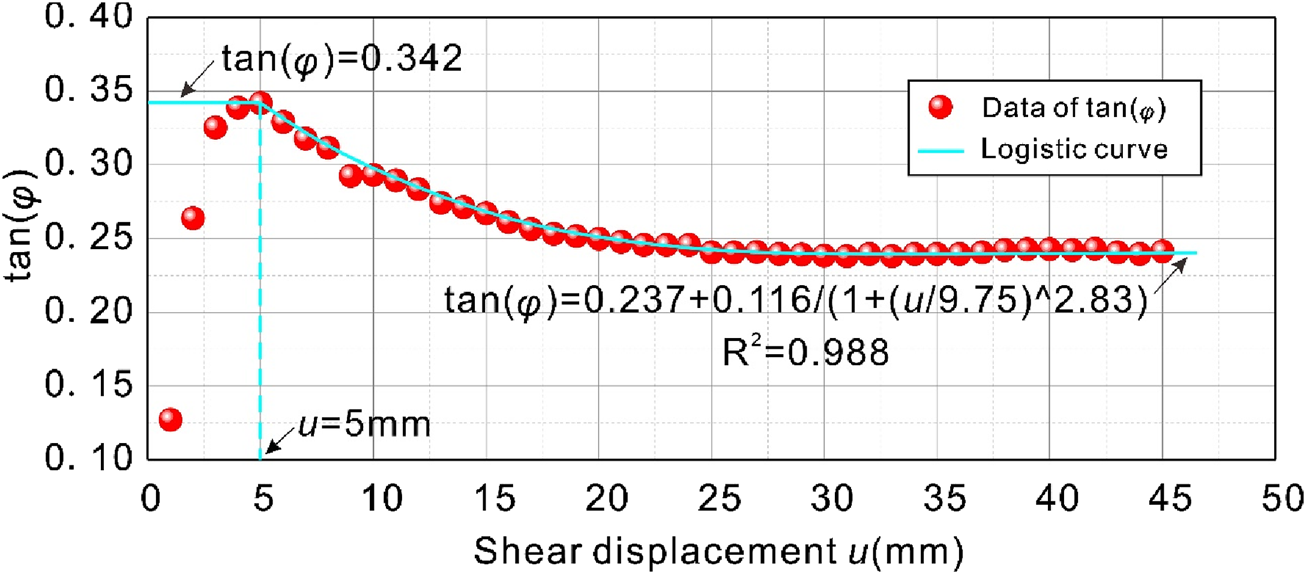
Evolution results of friction angle in slip zone soil.
Figure 6 shows the internal friction angle as a function of shear displacement. With the increase of shear displacement, the cohesion of the soil in the sliding zone is increasing rapidly, which indicates that the cohesion of soil particles in the sliding zone is resisting the external shear of the soil. After reaching the peak, the cohesion of the sliding zone soil decreases, indicating that the original stress structure in the sliding zone soil is continuously destroyed during the shearing process until the structural property is completely lost. The peak cohesion of the slip zone soil was 40.475 kPa, and the residual cohesion was constantly decreasing. In order to quantitatively evaluate the attenuation law of cohesion in the slip zone, the power function model was used for nonlinear fitting, and it can be seen from the results of Figure 6 that the fitting degree is 0.94, and the fitting effect is good, indicating that the attenuation law of cohesion obeys the power function change relationship.
FIGURE 6
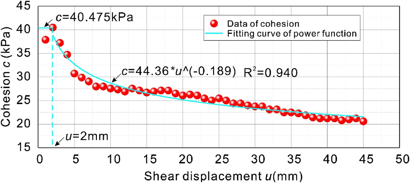
Evolution results of cohesion in slip zone soil.
3.5 The evolutionary law of shear strength in slip zone
In general, the results of the change of internal friction angle and cohesion are first increased and then decayed. Considering that the internal friction angle and cohesion essentially represent the strength of the soil and have nothing to do with the shear evolution process of the soil, the plastic hardening process before the peak internal friction angle and the peak cohesion is appropriately corrected, and the correction results are shown in Figures 5, 6. Correspondingly, according to the evolution fitting curve of friction angle and cohesion in the slip zone soil, combined with the Moore-Coulomb formula, the shear strength curve of the slip zone soil under the action of arbitrary normal stress can be obtained. Firstly, according to the evolution model of friction angle and cohesion in the soil of the sliding zone, as shown in Equation 1 and Equation 2:
Secondly, by substituting Equation 1 and Equation 2 into Equation 3, the dynamic variation model of shear strength of slip zone soil can be obtained:
According to the above steps, the shear strength of the sliding zone soil under normal stress of 100 kPa, 200 kPa, 300 kPa, 400 kPa, 500 kPa and 600 kPa was plotted with shear displacement, as shown in Figure 7. With the increase of normal stress, the shear strength increases, the attenuation amplitude of shear strength from peak strength to residual strength increases, the longer the strain softening state lasts, the greater the deformation needs to be constant, and the peak strength decays to the residual strength needs to experience greater displacement. The above process can obtain the shear strength value of slip zone soil through shear displacement under arbitrary normal stress, which lays a foundation for the study of landslide dynamic stability from the perspective of strength.
FIGURE 7
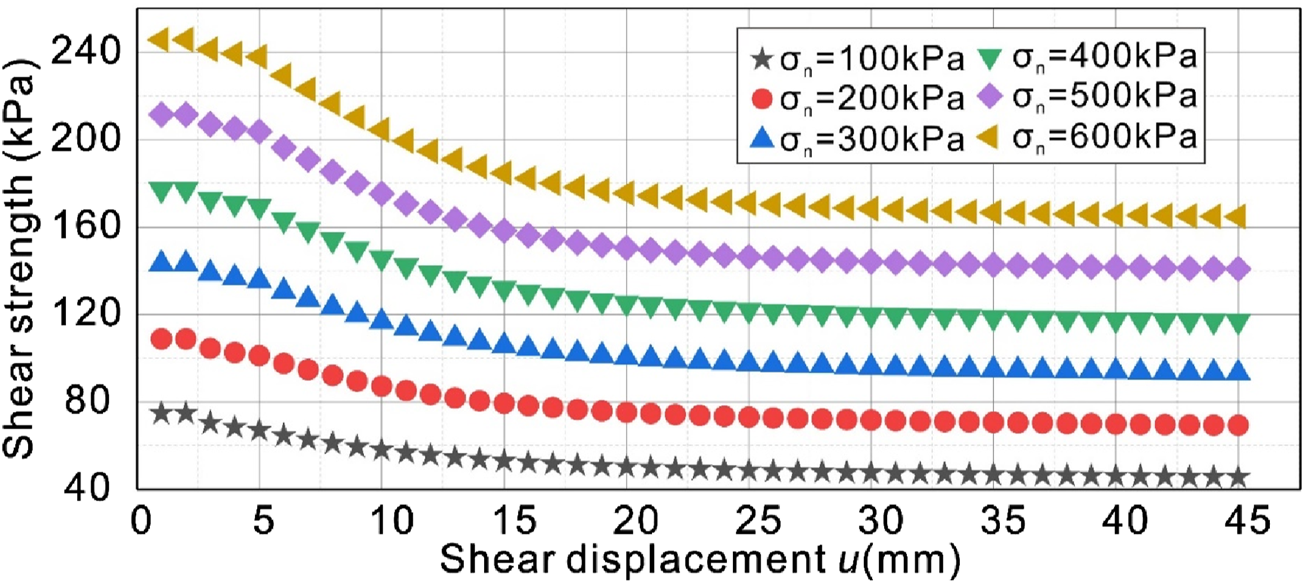
Dynamic evolution of shear strength of slip zone.
4 Landslide stability calculations
4.1 Landslide stability calculation process
Based on the dynamic variation curve of shear strength of the sliding zone obtained by the Moore-Coulomb theory, combined with the typical residual thrust method (Song and Xu, 2012), the improved mechanical model of landslide stability is established. In addition, the finite element numerical calculation model of the landslide was established by using the Geo-studio finite element software, and the dynamic stability evaluation of the landslide was compared and studied. The specific solution is divided into two aspects and the calculation process of landslide stability is shown in Figure 8.
FIGURE 8

Flow chart for the calculation of landslide dynamic stability.
The improved mechanical model of landslide stability: 1) The basic geometric parameters of the strip are obtained by the strip of the sliding body, including the width of the strip li, the volume of the strip Vi, the inclination angle αi at the bottom of the strip, and the effective average gravity γ and gravity Wi of the strip. 2) under the static equilibrium condition of any bar i along the direction of the vertical sliding surface, the normal stress σni of the vertical sliding surface of the bar and the partial gliding force Ti along the sliding surface are obtained; Based on the shear strength curve of the sliding belt based on the mol-Coulomb strength criterion under different normal stress conditions, the dynamic value of the shear strength of the shear belt at the bottom of the i block with shear displacement is obtained, and the dynamic anti-slip force value Ri of the i block along the sliding surface is obtained. 3) the difference between the sliding force Ti of any block i and the anti-sliding force Ri after the strength reduction is used to obtain the recursive equation of the residual thrust of the i block of the landslide, see Equations 4, 5; 4) Set the reduction factor Fr, and then solve the residual thrust of each block in turn, so that the residual thrust of the last block is equal to or close to 0, that is, the landslide stability calculation converges.
Numerical calculation model of finite element: 1) Establish a two-dimensional finite element numerical model of landslide, assign material parameters of sliding body and bedrock, set boundary conditions, and mesh the model; 2) The friction angle and cohesion weakening value in the soil in the slip zone were selected as the corresponding representative landslide deformation conditions to assign the strength parameters of the slip zone, and the numerical simulation analysis of landslide deformation and failure was carried out. 3) The contour of the landslide deformation evolution result and the dynamic stability coefficient of the landslide are stopped until the stability coefficient of the landslide remains stable, indicating that the calculation of the stability of the landslide is convergent.
4.2 A mechanical model of landslide stability based on the evolution of friction angle and cohesion
Based on the dynamic evolution model of mol-Coulomb strength and the typical residual thrust method, a computational mechanical model of landslide stability with dynamic changes of internal friction angle and cohesion force is established. With the change of shear displacement, the friction angle and cohesion in the slip zone also change, and the shear strength will also weaken, so the landslide thrust and stability calculated by the model will have a dynamic evolution. The 2–2 section of the landslide was selected as the typical section for strip calculation. Taking any bar i as the research object for specific analysis, as shown in Figure 9, according to the overall force balance condition along the sliding surface of any bar i, the residual thrust Pi of any bar i is:where Pi-1 is the residual thrust of bar i-1; αi-1 and αi represent the horizontal dip angles of the bottom sliding surface at bar i-1 and i, respectively, and the inclination angle of the sliding surface of the reverse warping section is negative. Wi is the weight of strip i, and severe γi is taken as natural severity. Fr is the strength reduction factor, also known as the safety factor for landslide stability calculation, it is the critical value for a landslide to maintain the ultimate equilibrium state; τsi is the shear strength of the sliding zone at the bottom of the bar, which can be obtained from the dynamic evolution model of mol-coulomb strength. li is the length of the bottom of bar i; hi is the average height of bar i.
FIGURE 9
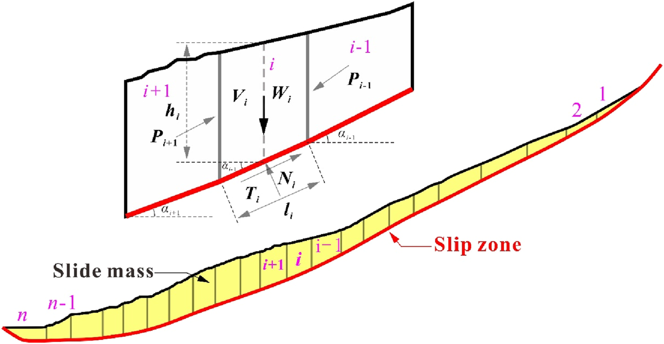
Force diagram of slide mass.
From the static equilibrium condition perpendicular to the bottom of bar i, it can be seen that the normal stress at the bottom of bar i becomes:
4.3 Landslide applications
In the landslide stability analysis, it is generally considered that the landslide speeds do not detach and overlap with each other, that is, the horizontal displacement of each block is equal by default (Zhang and Wang, 2010), that is, the displacement between adjacent blocks satisfies as shown in Equation 6.where ui and ui-1 are the displacements of bar and i-1, respectively, and αi and αi-1 are the inclination angles of bar i and bar i-1, respectively.
4.4 Numerical simulation comparison
The 2–2 section of the landslide was selected as the typical geological section, and the two-dimensional numerical calculation model of the landslide was established by the Geo-Studio finite element software, as shown in Figure 10. According to the spatial structure of the landslide, the landslide is divided into three materials, the ideal elastoplastic model is used for the sliding body and the sliding belt material, and the ideal elastic model is used for the bedrock sliding bed. In order to accurately reveal the deformation and failure of the landslide, the mesh near the slip zone material was further subdivided, and a total of 6482 grid elements and 6541 grid nodes were divided. According to the results of indoor physical and mechanical tests and geotechnical engineering investigations, the physical and mechanical calculation parameters of each layer of the numerical calculation model are comprehensively determined, as shown in Table 3.
FIGURE 10
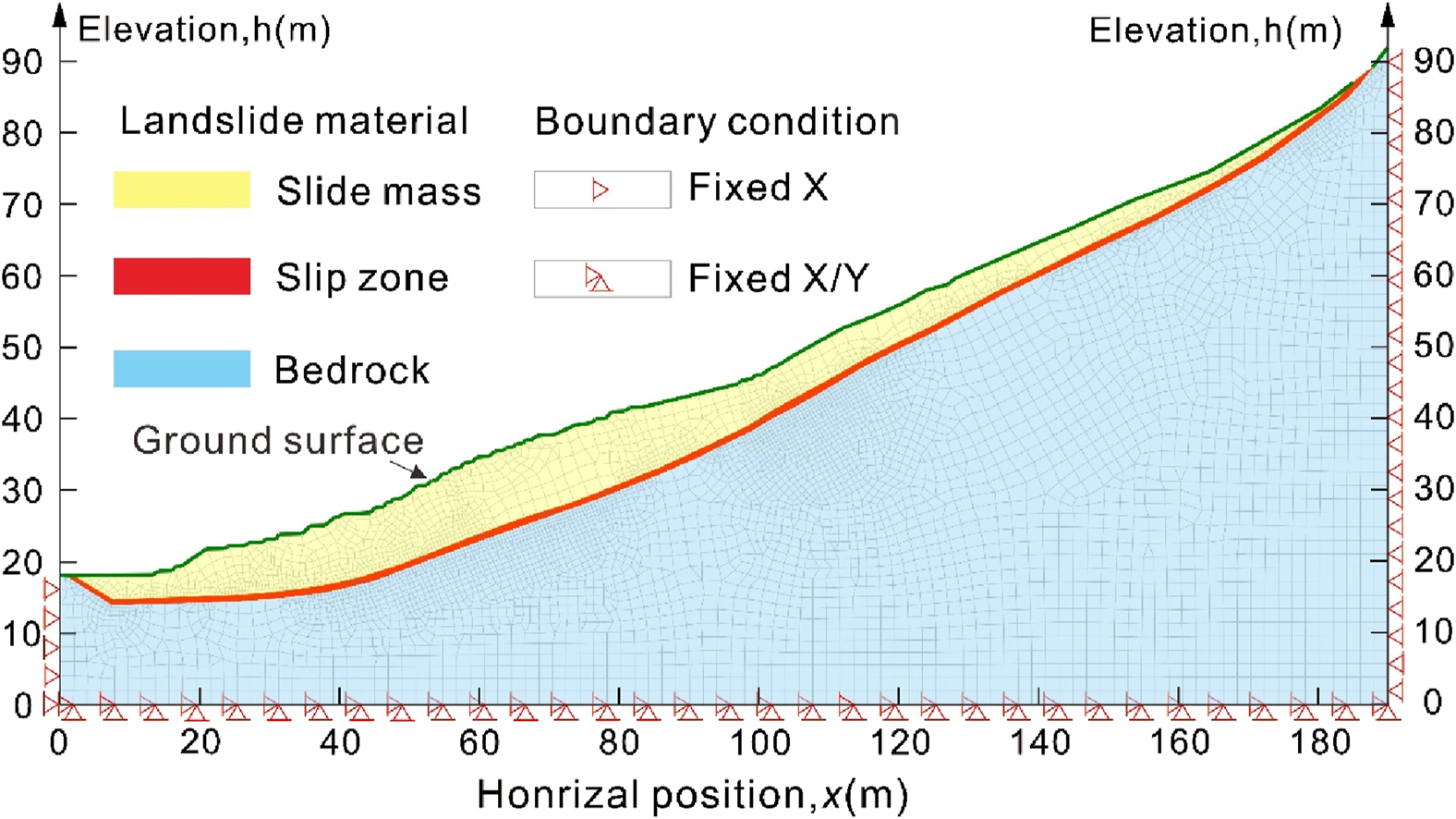
Numerical calculation model.
TABLE 3
| Landslide structures | Material composition | Internal friction angle (°) | Cohesion c (kPa) | Gravity (kN/m3) | Elastic modulus E (kPa) | Poisson ratio u |
|---|---|---|---|---|---|---|
| Slide mass | Crushed stones and blocks | 22 | 28 | 19 | 40 | 0.35 |
| Slip zone | Silty clay | — | — | 18.5 | 20 | 0.2 |
| Bedrock | Sandy slate | 40 | 45 | 27 | 45 | 0.4 |
Mechanical parameters of the finite element numerical model of landslide.
In order to accurately and comprehensively reveal the results of landslide deformation evolution, the internal friction angle and cohesion weakening values of six groups of slip zone soils were selected as the corresponding representative landslide deformation conditions for numerical simulation analysis, and the specific scheme is shown in Table 4.
TABLE 4
| Condition | Friction angle of slip zone (°) | Cohesion of slip zone c (kPa) | Shear displacement u (mm) |
|---|---|---|---|
| (a) | 18.85 | 37.874 | 1 |
| (b) | 18.85 | 30.714 | 5 |
| (c) | 16.33 | 27.549 | 10 |
| (d) | 14.96 | 26.706 | 15 |
| (e) | 14.04 | 26.073 | 20 |
| (f) | 13.41 | 23.752 | 30 |
Simulating conditions.
5 Results
5.1 Evolution results of shear strength distribution of slip zone
With the evolution of landslide, the shear displacement of slip zone also shows a trend of weakening in space. In order to quantitatively reveal the weakening degree of the strength of slip zone, the relationship between the strength of the bottom of slide mass and the shear displacement was calculated and analyzed. Figure 11 shows the spatial distribution of slip zone strength at each position at the bottom of the landslide and the variation with shear displacement.
FIGURE 11

Evolution results of dynamic distribution of shear strength in slip zone.
Spatially, from the trailing edge to the front edge of the landslide, the strength distribution of slip zone generally shows a pattern of first increasing and then decreasing, and the strength of slip zone is the highest at 139.6 m. In the middle part of the 139.6 m sliding body, the thickness of slide mass is the deepest, reaching a maximum depth of 10.9 m, extending to the front edge and the trailing edge, the thickness of slide mass is about thin, and the buried depth of slip zone is shallow. The deeper the slip zone is embedded, the greater the normal stress, and the greater the shear strength of slip zone, and vice versa. It is worth noting that the strength of the leading edge of slip zone increases abruptly, which is due to the reverse warping of the dip angle of slip zone, which increases the normal stress of slip zone, resulting in an increase in strength.
In terms of time, the strength of slip zone showed a gradual trend. With the increase of landslide displacement, the peak strength of slip zone gradually decays, and the strain softening begins to occur in slip zone, which gradually tends to be stable after about 25 mm, and remains in their respective residual strength states.
With the continuous increase of landslide displacement, the shear strength at each slip zone is strained and softened and attenuated to different degrees, and the deeper the buried depth of the slip zone, the greater the normal stress of the upper sliding body, and the faster the shear strength attenuation of the slip zone.
5.2 Evolution results of landslide deformation and failure process
By means of numerical simulation, the different attenuation values of friction angle and cohesion in slip zone are taken as the deformation conditions, and the deformation displacement of the landslide and the maximum shear strain increment of slip zone are taken as the evaluation indexes, and the deformation evolution mechanism of the landslide is analyzed through dynamic calculation. The trailing edge of the landslide.
Figure 12 shows the evolution contour of landslide deformation under different shear displacement conditions. With the attenuation of the strength index of slip zone, the deformation evolution of the landslide gradually intensifies. When the shear displacement of slip zone is 1 mm, the deformation of the landslide is mainly manifested in the leading edge and the trailing edge, and the middle part is almost not deformed. With the increasing shear displacement, the friction angle and cohesion in slip zone are continuously attenuated, and the deformation of the landslide is intensified, and the deformation of the leading and trailing edges of the landslide extends to the middle part. When the shear displacement reaches 30 mm, the friction angle and cohesion in slip zone are stabilized in their respective residual states, and the landslide produces an overall sliding. The simulation results show the deformation of the front and trailing edges, and then extend the deformation to the middle sliding body, which is consistent with the deformation and failure signs of the collapse of the trailing edge due to the steep slope and the slip of the leading edge due to river erosion and cutting. The simulation results can accurately reveal the deformation evolution process of the landslide.
FIGURE 12

The evolution process of landslide deformation displacement. (a) c=37.874kPa and φ=18.85°; (b) c=30.714kPa and φ=18.85°; (c) c=27.549kPa and φ=16.33°; (d) c=26.706kPa and φ=14.96°; (e) c=26.073kPa and φ=13.94°; (f) c=23.752kPa and φ=13.41°.
Figure 13 shows the incremental evolution of shear strain in slip zone under different deformation states of the landslide. As shown in Figure 13, with the attenuation of friction angle and cohesion in slip zone, the shear failure of slip zone is gradually penetrated. The shear strain increment of slip zone has a good correspondence with the deformation and displacement evolution state of the landslide. When the shear displacement is 1 mm, the shear strain of slip zone is sporadically distributed at the leading and trailing edges of the landslide, and the shear strain in the middle of the slip zone is not penetrated, so the leading edge of the landslide shows traction slip, and the trailing edge of the landslide shows stacked deformation. With the increasing shear displacement, the shear strain of the slip zone expands from both sides to the middle, and the landslide gradually shows a trend of gradual failure. When the shear displacement reaches 30 mm, the shear strain is integrated through, and the landslide manifests as overall deformation and failure.
FIGURE 13

Evolution of the maximum shear strain increment. (a) c=37.874kPa and φ=18.85°; (b) c=30.714kPa and φ=18.85°; (c) c=27.549kPa and φ=16.33°; (d) c=26.706kPa and φ=14.96°; (e) c=26.073kPa and φ=13.94°; (f) c=23.752kPa and φ=13.41°.
5.3 Evolution results of landslide dynamic stability
The improved stability computational mechanical model and finite element numerical calculation model were used to obtain the dynamic stability of the landslide, respectively. Figure 14 shows the evolution of landslide stability as a function of displacement. As shown in Figure 14, the stability calculated by the two models has the same evolutionary law and the difference is small, and both gradually decrease from peak stability to residual stability. In the initial sliding state of the landslide, the peak stability of the landslide is 1.25, with the increase of the landslide displacement, the strain of slip zone begins to soften, the strength is gradually weakened, the anti-sliding force of the landslide gradually decreases, and the stability of the landslide gradually decreases from the peak; when the strain softening phenomenon of slip zone is over, the shear strength of slip zone is stable at the respective residual strength, and the landslide is gradually stabilized in the residual state, and the residual stability is between 1.07 and 1.08.
FIGURE 14
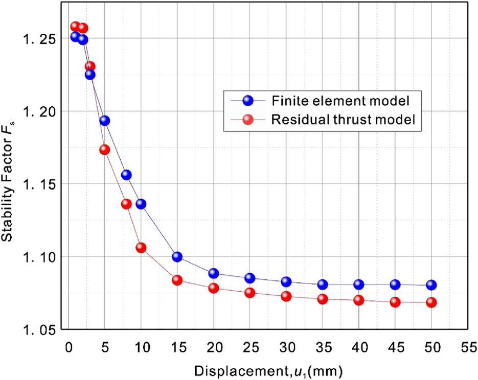
Stability evolution of landslide.
The residual stability of the landslide is between 1.07 and 1.08, indicating that the landslide is currently in a basically stable state. The stability of the landslide changes from time to time, and it is possible to slide again in the later stage of the landslide under the induction of a combination of rainfall infiltration, river erosion at the front edge and steep slope at the back edge. Therefore, the trailing edge of the landslide should be appropriately cut and the leading edge of the landslide should be diverted. In addition, necessary measures such as monitoring and early warning should be carried out irregularly in the later stage, especially in the high incidence of the local rainy season, so as to prevent large-scale landslide sliding under heavy rainfall infiltration conditions and ensure the normal operation of highway traffic.
In this study, the samples in slip zone soil were screened with coarse particles, and the fine particles were retained. In its actual state, the slip zone soil is accompanied by a large number of coarse grains. Therefore, the shear strength of slip zone soil tested by the ring shear test is obviously weaker than that of the actual slip zone soil, and the calculation results of landslide stability are also low. Therefore, the ring shear test in situ can be carried out in order to obtain a more accurate shear strength of slip zone soil and accurately analyze the stability evaluation of the landslide.
6 Conclusion
In this paper, the on-site engineering geological investigation of a high-speed subgrade landslide is carried out, the soil samples of the slip zone are taken, the ring shear test is carried out, and the dynamic model of the strength of the slip zone with the change of internal friction angle and cohesion is established by combining the Moore Coulomb theory. Secondly, the dynamic model of sliding belt strength was combined with the typical residual thrust method to establish an improved computational mechanical model of landslide stability. Finally, the finite element model of the landslide was established by using the Geo-studio finite element software, and the deformation evolution mechanism of the landslide with the weakening of the friction angle and cohesion in the slip zone was analyzed. The following conclusions are drawn:
(1) The deformation and failure evolution mechanism of landslide is revealed. Through the on-site engineering geological investigation, it is shown that the slip shows a collapse-figure slip failure. The numerical simulation results show that with the increase of sliding displacement, the deformation displacement of the landslide gradually increases and expands from the leading edge and trailing edge to the middle, and the shear strain of the slip zone gradually penetrates from the leading edge and the trailing edge deformation, which is consistent with the phenomenon revealed by the field engineering geological investigation.
(2) The results of the attenuation of the shear strength of the slip belt are obtained. The friction angle in the soil in the slip zone shows a law with the attenuation of the logistic model, and the cohesion force shows a law with the attenuation of the power function model. The strength of the sliding belt gradually decreases in the middle and the front and back edges, and the strength of the sliding belt is the highest at 119.4 m, and the distribution on both sides of the front and trailing edges decreases gradually. With the evolution of the landslide displacement, the strength values of each slip zone show strain softening, and finally stabilize at their respective residual strengths.
(3) The evolution results of landslide dynamic stability were evaluated. With the increase of landslide displacement, the stability of the landslide gradually decreases from the peak stability to the law of their respective residual stability, and the difference between the stability calculated by the two mechanical models is small.
Statements
Data availability statement
The original contributions presented in the study are included in the article/supplementary material, further inquiries can be directed to the corresponding author.
Author contributions
YD: Conceptualization, Writing – original draft. MZ: Writing – original draft, Data curation, Methodology. TL: Writing – review and editing, Investigation. YZ: Formal Analysis, Methodology, Writing – review and editing.
Funding
The author(s) declare that financial support was received for the research and/or publication of this article. This research was funded by Natural Science Foundation of Jiangxi Province (20232BAB214069).
Acknowledgments
The authors would like to thank the reviewers of this paper for their constructive comments.
Conflict of interest
The authors declare that the research was conducted in the absence of any commercial or financial relationships that could be construed as a potential conflict of interest.
Generative AI statement
The author(s) declare that no Generative AI was used in the creation of this manuscript.
Publisher’s note
All claims expressed in this article are solely those of the authors and do not necessarily represent those of their affiliated organizations, or those of the publisher, the editors and the reviewers. Any product that may be evaluated in this article, or claim that may be made by its manufacturer, is not guaranteed or endorsed by the publisher.
References
1
Chen X. Ren J. Wang D. Lyu Y. Zhang H. (2019). A generalized strength reduction concept and its applications to geotechnical stability analysis. Geotech. Geol. Eng.37, 2409–2424. 10.1007/s10706-018-00765-1
2
Chen X. P. Liu D. (2014). Residual strength of slip zone soils. Landslides11 (2), 305–314. 10.1007/s10346-013-0451-z
3
Chen X. P. Zhu H. H. Huang J. W. Liu D. (2016). Stability analysis of an ancient landslide considering shear strength reduction behavior of slip zone soil. Landslides13 (1), 173–181. 10.1007/s10346-015-0629-7
4
Geng Z. Jin D L. Yuan D J. (2023). Face stability analysis of cohesion-frictional soils considering the soil arch effect and the instability failure process. Comput. Geotech.153, 105050. 10.1016/j.compgeo.2022.105050
5
Hua C. Zou Z. Fan M. Duan H. Niu Y. Jiang Z. (2025). DEM parameter calibration strategy applied to the strain-softening characteristics of sliding zone soil with the support of GA-BP. Powder. Technol.457, 120880. 10.1016/j.powtec.2025.120880
6
Li W. Yang Q. (2018). Hydromechanical constitutive model for unsaturated soils with different overconsolidation ratios. Int. J. Geomech.18 (2), 04017142. 10.1061/(asce)gm.1943-5622.0001046
7
Li Y. J. Xie Q. L. (2013). Study on discriminant criterion of highway landslide disaster. Appl. Mech. Mater275, 2735–2739. 10.4028/www.scientific.net/amm.275-277.2735
8
Liu D. Chen X. (2015). Shearing characteristics of slip zone soils and strain localization analysis of a landslide. Geomec. Eng.8 (1), 33–52. 10.12989/gae.2015.8.1.033
9
Liu X. L. Yang J. J. (2011). An approach for landslide stability evaluation by numerical method. Key. Eng. Mater.462, 42–47. 10.4028/www.scientific.net/kem.462-463.42
10
Luo Y. Zou Z. Li C. Duan H. Thaw N. M. M. Zhang B. et al (2022). Analysis of shear constitutive models of the slip zone soil based on various statistical damage distributions. Appl. Sci.12 (7), 3493. 10.3390/app12073493
11
Nian T. K. Feng Z. K. Yu P. C. Wu H. J. (2013). Strength behavior of slip-zone soils of landslide subject to the change of water content. Nat. Hazards68, 711–721. 10.1007/s11069-013-0647-5
12
Sarkar S. Pandit K. Dahiya N. Chandna P. (2021). Quantified landslide hazard assessment based on finite element slope stability analysis for uttarkashi–gangnani highway in Indian himalayas. Nat. Hazards106, 1895–1914. 10.1007/s11069-021-04518-x
13
Song Z. F. Xu X. M. (2012). Brief introduction of residual thrust method and its improvement. Appl. Mech. Mater.166, 3358–3363. 10.4028/www.scientific.net/amm.166-169.3358
14
Su A. Feng M. Dong S. Zou Z. Wang J. (2022). Improved statically solvable slice method for slope stability analysis. J. Earth. Sci.33 (5), 1190–1203. 10.1007/s12583-022-1631-3
15
Thaw N. M. M. Li C. Zou Z. Chen W. Long J. Oo A. M. et al (2025). Shearing characteristics of Jurassic silty mudstone slip zone under different water contents and normal stresses based on ring shear tests. J. Earth. Sci.36 (2), 654–667. 10.1007/s12583-022-1762-6
16
Wang L. Han J. Liu S. Yin X. (2020). Variation in shearing rate effect on residual strength of slip zone soils due to test conditions. Geotech. Geol. Eng.38, 2773–2785. 10.1007/s10706-020-01186-9
17
Wang R. Yan H. Yao J. Li Z. (2024). Stability analysis of slopes under seismic action with asynchronous discounting of strength parameters. Appl. Sci.15 (1), 169. 10.3390/app15010169
18
Wu S. Han L. Cheng Z. Zhang X. Cheng H. (2019). Study on the limit equilibrium slice method considering characteristics of inter-slice normal forces distribution: the improved spencer method. Environ. Earth. Sci.78, 611. 10.1007/s12665-019-8621-5
19
Yan J. Kong L. Chen C. Guo M. (2024). A vector sum analysis method for stability evolution of expansive soil slope considering shear zone damage softening. J. Rock Mech. Geotech. Eng.16 (9), 3746–3759. 10.1016/j.jrmge.2024.04.009
20
Yan J. Zou Z. Mu R. Hu X. Zhang J. Zhang W. et al (2022). Evaluating the stability of outang landslide in the three gorges reservoir area considering the mechanical behavior with large deformation of the slip zone. Nat. Hazards112 (3), 2523–2547. 10.1007/s11069-022-05276-0
21
Yang B. B. Chen Y. Yuan S. C. (2024a). Investigation on structure, evaporation, and desiccation cracking of soil with straw biochar. Land. Degrad. Dev.35 (9), 3126–3135. 10.1002/ldr.5122
22
Yang B. B. Chen Y. Zhao C. Li Z. L. (2024b). Effect of geotextiles with different masses per unit area on water loss and cracking under bottom water loss soil conditions. Geotext. Geomembranes52, 233–240. 10.1016/j.geotexmem.2023.10.006
23
Yu M. (2020). Analysis on stability of Mountain mass and numerical calculation of landslide resistance based on strength reduction method. Arab. J. Geosci.13 (14), 617. 10.1007/s12517-020-05617-y
24
Zhang G. Wang L. (2010). Stability analysis of strain-softening slope reinforced with stabilizing piles. J. Geotech. Geoenviron. Eng.136 (11), 1578–1582. 10.1061/(asce)gt.1943-5606.0000368
25
Zou Z. Luo T. Tan Q. Yan J. Luo Y. Hu X. (2023a). Dynamic determination of landslide stability and thrust force considering slip zone evolution. Nat. Hazards118 (1), 31–53. 10.1007/s11069-023-05992-1
26
Zou Z. Luo T. Zhang S. Duan H. Li S. Wang J. et al (2023b). A novel method to evaluate the time-dependent stability of reservoir landslides: exemplified by outang landslide in the three gorges reservoir. Landslides20 (8), 1731–1746. 10.1007/s10346-023-02056-0
27
Zou Z. Luo Y. Tao Y. Wang J. Duan H. (2024). Shear constitutive model for various shear behaviors of landslide slip zone soil. Landslides21 (12), 3087–3101. 10.1007/s10346-024-02345-2
28
Zou Z. Yan J. Tang H. Wang S. Xiong C. Hu X. (2020). A shear constitutive model for describing the full process of the deformation and failure of slip zone soil. Eng. Geol.276, 105766. 10.1016/j.enggeo.2020.105766
Summary
Keywords
landslide, slip zone soil, shear strength, landslide dynamic stability, friction-cohesion
Citation
Deng Y, Zhao M, Luo T and Zhou Y (2025) Deformation mechanism and dynamic stability of the subgrade landslide considering evolution of friction-cohesion in slip zone. Front. Earth Sci. 13:1650860. doi: 10.3389/feart.2025.1650860
Received
20 June 2025
Accepted
22 July 2025
Published
12 August 2025
Volume
13 - 2025
Edited by
Binbin Yang, Xuchang University, China
Reviewed by
Zihua Cheng, Sun Yat-sen University, China
Jun-Wei Bi, Shandong Jiaotong University, China
Updates
Copyright
© 2025 Deng, Zhao, Luo and Zhou.
This is an open-access article distributed under the terms of the Creative Commons Attribution License (CC BY). The use, distribution or reproduction in other forums is permitted, provided the original author(s) and the copyright owner(s) are credited and that the original publication in this journal is cited, in accordance with accepted academic practice. No use, distribution or reproduction is permitted which does not comply with these terms.
*Correspondence: Tao Luo, 18296760919luotao@cug.edu.cn
Disclaimer
All claims expressed in this article are solely those of the authors and do not necessarily represent those of their affiliated organizations, or those of the publisher, the editors and the reviewers. Any product that may be evaluated in this article or claim that may be made by its manufacturer is not guaranteed or endorsed by the publisher.