Abstract
Calcareous sand is widely used as fill material in island construction projects in the South China Sea. The mechanical properties of the interface between calcareous sand and geogrid under high temperatures and complex environmental conditions play a critical role in the long-term stability of such structures. In this study, interfacial pullout tests between calcareous sand and a geogrid are conducted under six temperature conditions (−5 °C, 0 °C, 20 °C, 40 °C, 60 °C, and 80 °C) and various normal stress levels. A database containing 1178 data sets is established from these tests. Based on the test data, four predictive models are developed: support vector machine (SVM), particle swarm optimization SVM (PSO-SVM), genetic algorithm optimization SVM (GA-SVM), and a deep learning long short-term memory network (LSTM). The results indicate that the LSTM model provides significantly higher predictive accuracy and robustness compared to traditional machine learning models, achieving an R2 value of 0.97 on both training and testing datasets and superior performance in RMSE, MAPE, MAE, and MSE. Sensitivity analysis using SHAP values shows that shear displacement has the greatest influence on shear strength, followed by temperature, normal stress, and particle size. Furthermore, based on the LSTM model predictions, an empirical formula for shear strength is proposed, enabling engineers without expertise in deep learning to estimate the shear strength of calcareous sand–geogrid interfaces effectively.
1 Introduction
The South China Sea (SCS) is an important international shipping channel and a resource-rich region. In recent years, the construction of islands and reefs in this area has been gradually promoted. Large-scale reclamation projects often use calcareous sand as the primary filling material (Chao et al., 2023a; Wang et al., 2022). Calcareous sand is susceptible to significant deformation and particle breakage under external loading. This behavior poses challenges to the long-term stability of island structures (Shao et al., 2024; Zhao et al., 2025). To enhance the stability of calcareous sand foundations, geosynthetic reinforcement technology has been applied (Fan et al., 2023). Nevertheless, the South China Sea has a high temperature climate and a large number of high-temperature oil and gas pipelines are laid on the seabed, and the temperature changes are significant and complex (Luo et al., 2024; Shi et al., 2023). The high-temperature environment not only affects the structural rearrangement and strength parameters of the calcareous sand particles but also significantly weakens the mechanical properties of the polymer-based geogrid (Zhang Y. et al., 2023), which in turn alters the mechanical response of the calcareous sand-geogrid interface (CSGI, hereafter) (Zhao G. et al., 2023; Zhou Y. et al., 2022). Therefore, it is of great significance to study the mechanical properties of the CSGI under temperature change to ensure the long-term service performance and structural safety of the SCS islands and reefs project.
The direct test of pullout under temperature-controlled conditions is an effective method to evaluate the mechanical properties of CSGI. It has been shown that temperature has a significant effect on interfacial mechanical behaviour (Zhao S. et al., 2023; Zheng et al., 2024a). Lin et al. (2024) reported that the shear strength of the GMB/GTX interface reaches its maximum at 30 °C–40 °C, based on shear tests conducted between 10 °C and 70 °C (Lin et al., 2024). The displacement needed for the interface to reach its peak strength generally decreases as temperature increases (Dong et al., 2017). Ghazizadeh et al. carry shear tests at normal stresses ranging from 100 kPa to 2000 kPa and show that the temperature increase resulted in a decrease of up to 45% in the peak internal shear strength of the GCL, as well as a decrease in the values of its corresponding maximum displacements by 32% and 48%, respectively (Ghazizadeh and Bareither, 2024). It is also shown that in addition to the temperature factor, factors such as particle size, normal stress and shear displacement also significantly affect the interfacial mechanical behavior (Chao et al., 2024d; Chao et al., 2024e). Although the temperature-controlled pullout test can effectively reveal the mechanism of temperature influence on interfacial properties, the method still has some limitations (Ren et al., 2024). First, the test equipment needs to be equipped with a temperature control system, which greatly increases the test cost and operational complexity (Chao et al., 2024b). Second, reproducing the complex and significant temperature fluctuations of the marine environment in laboratory experiments remains a challenge (Chao et al., 2025). These fluctuations affect the mechanical properties of calcareous sand and geogrid, and they alter the behavior of the calcareous sand-geogrid interface (CSGI) (Wang et al., 2023). In addition, the cumulative damage effect of long-term temperature cycling on interfacial properties requires time-consuming experimental studies (Shu et al., 2025; Xu et al., 2024). Therefore, it is important to establish a prediction model that can comprehensively consider the temperature and other environmental factors to make up for the insufficiency of physical tests. Provide a more reliable design basis for the application of geosynthetics in marine engineering.
To make up for the shortcomings of traditional test methods, machine learning-based prediction modeling has become an important method for interface strength research. Among them, support vector machine (SVM) has been widely used in marine engineering prediction tasks due to its excellent performance in dealing with small-sample, nonlinear, and high-dimensional data problems (Chao et al., 2023b; Zhou B. et al., 2022). In the existing studies, SVM can effectively extract the nonlinear relationship between input variables such as temperature, normal stress (Chao et al., 2023c; Chao et al., 2024g), pullout displacement and shear strength and realize the prediction with higher accuracy (Chao et al., 2024a; Li et al., 2024). For example, Chao et al. demonstrate that SVM can successfully capture the complex interactions between variables like temperature, normal stress, shear stress, time, and interface displacement through temperature-controlled shear tests (Chao et al., 2023c; Chao et al., 2023d). Xie et al. use SVM to predict the shear strength of the rock interface (SSOTRI) (Xie et al., 2023; Zhang W. et al., 2023), achieving a high prediction accuracy with a relative error of just 3.2% and a correlation coefficient of 0.95 (Lin et al., 2024; Song et al., 2024). Nevertheless, the SVM model is sensitive to hyperparameters such as the kernel function parameters and the penalty factor (Chao et al., 2024c), and the model performance is easily affected (Cui et al., 2024). To improve the stability and accuracy of SVM, optimization algorithms such as particle swarm optimization (PSO) and genetic algorithm (GA) are employed, leading to models like PSO-SVM and GA-SVM(Cheng et al., 2023; Ding et al., 2024). Although these integrated models have improved the prediction performance to a certain extent, there are still many limitations (Chao et al., 2024f; Li et al., 2025). On the one hand, optimization algorithms such as GA may fall into local optimum in the convergence process, and PSO, although faster in convergence, is more sensitive to the initial population and parameter settings, and its searchability in high-dimensional data processing is relatively limited (Xiao and Xu, 2024). On the other hand, machine learning models usually rely on the manual selection of input features (Xiao et al., 2024). It relies too much on domain knowledge and empirical judgment, which can easily lead to the omission of feature information or the introduction of subjective bias (Huang et al., 2024). Affecting the comprehensiveness and reliability of the model. In addition, in the face of complex situations such as multivariate coupling, unsteady loading and dynamic temperature change (Qin et al., 2025; Wang et al., 2024). The expression ability of traditional machine learning models is still limited. Their generalization performance is also insufficient to meet the high-precision requirements for predicting interface behaviors in real engineering applications (Zheng et al., 2024b; Zheng et al., 2024c). Therefore, to further enhance the automation and modeling capability of interface mechanical property prediction, deep learning methods have been gradually adopted. These methods enable automatic extraction of features and processing of high-dimensional data.
The introduction of deep learning techniques provides new ideas for the prediction of interface mechanical behavior. As a recurrent neural network structure that can effectively process time-series data and capture long-term dependencies (Fan et al., 2025). The deep learning Long Short-Term Memory (LSTM) network has been gradually applied to the modeling of geotechnical engineering problems in recent years (Shu et al., 2025). Compared with machine learning SVM-like models, LSTM is not only capable of learning complex nonlinear relationships but also dynamically responds to the changing characteristics of input variables over time or loading process, which is suitable for data modeling tasks with time-series characteristics, such as temperature, displacement, etc .,(Ye et al., 2019). Yang et al. establish the LSTM model to be used to predict the bond strength at the rebar - concrete interface in recycled aggregate concrete under the conditions of different reinforcing bar types, water - cement ratios and substitution rates of recycled aggregates (Yang et al., 2025). The results show that the model performs superiorly in dealing with high - dimensional features and time - series data and is able to capture the nonlinear variation characteristics of the bond strength more accurately (Ye et al., 2022). Chen et al. developed an LSTM model for the bond strength of artificial frozen soil-structure interfaces under different conditions of soil moisture content, positive pressure, and temperature (Chen et al., 2022). The shear behavior of an artificially frozen soil-structure interface verifies its effectiveness in dynamically simulating the evolution of the interface stress-displacement relationship in the prediction of interface mechanical behavior (Gao and Ye, 2023). Gao et al. combine metal intrusion techniques, BSE imaging, and the ResNet50 algorithm to identify historical high-temperature deterioration of sandstone. The results show that deep learning is feasible for analyzing microscopic thermal effects in high-temperature rocks (Gao and Ye, 2024). Sakcali et al. use deep learning models such as AdaBoost to predict the physical and mechanical properties of rocks under freeze–thaw and thermal shock cycles. The study shows that deep learning can efficiently quantify the effects of thermal actions on rock properties (Sakcali, 2024). Liu et al. employ a U-Net network to identify fissure parameters at the pixel level in freeze–thaw sandstone. The study verifies that deep learning is applicable for geotechnical analysis under freeze–thaw conditions (Liu et al., 2025). LSTM captures the evolution law of interface response by learning the historical loading path and temperature change process and then realizes the dynamic prediction of shear strength under different loading stages (Gao et al., 2024; Ye and Gao, 2024). By constructing a prediction model based on LSTM and combining it with experimental data for training and validation, not only the prediction accuracy can be effectively improved (Gong et al., 2025a; Gong et al., 2025b), but also the limitations of the experimental means and the traditional model’s insufficient simulation of the actual environment can be overcome.
In this study, the mechanical response of the calcareous SGI under different temperatures and normal stress conditions is systematically analyzed. By conducting interface pullout tests under the conditions of calcareous sand with particle sizes of 0.25–1 mm, 1–2 mm and 2–4 mm, several sets of shear strength data under the combination of temperature and stress are obtained, and a database is established based on the test results. On this basis, various prediction models, including traditional machine learning models and the deep learning LSTM model, are constructed to model and predict the interfacial shear strength. The comparative analysis ultimately reveals that the LSTM model provides the highest predictive accuracy and robustness, significantly outperforming the traditional machine learning models.
2 Materials and methods
2.1 Materials
As shown in Figure 1, the experimental materials are calcareous sand and geogrid. To examine the interfacial mechanical characteristics as affected by particle size variation, the calcareous sand is categorized into three groups of particle sizes according to the ASTM D6706 standard sieving method. Particle sizes between 0.25–1 mm, 1–2 mm, and 2–4 mm are referred to as S1, S2, and S3, respectively, for subsequent characterization. Figure 1B shows the scanning electron microscope (SEM) image of calcareous sand, through which the morphological characteristics and surface roughness of the particles can be observed. The physical parameters corresponding to the different calcareous sand groups are shown in Table 1. Figure1C shows the scanning electron microscope (SEM) image of calcareous sand. Through this image, the morphological characteristics and surface roughness of the particles can be observed. This experiment employs TGSG 40–40 polyethylene bidirectional geogrid as the reinforcement material, with its appearance shown in Figure 1B. This geogrid model features a uniform and stable grid structure with high tensile strength in both directions. Its primary physical parameters are detailed in Table 2.
FIGURE 1

Experimental material. (A) S1, S2, S3 calcareous sand. (B) geogrid. (C) SEM electron microscope scans.
TABLE 1
| Sand sample | Particle size (mm) | Specific gravity | Density (g/cm3) | D50 | Cu | Cc | e min | e max |
|---|---|---|---|---|---|---|---|---|
| S1 | 0.25–1 | 2.81 | 1.43 | 0.43 | 1.71 | 0.86 | 0.75 | 1.12 |
| S2 | 1–2 | 2.81 | 1.27 | 1.17 | 1.16 | 1.11 | 0.77 | 1.26 |
| S3 | 2–4 | 2.81 | 1.19 | 3 | 1.38 | 0.96 | 0.81 | 1.42 |
Basic physical parameters of test sand samples.
TABLE 2
| Parameters | Value |
|---|---|
| Ultimate Strength of Longitudinal Ribs (kN/m) | 51.17 |
| Ultimate strength of transverse ribs (kN/m) | 53.86 |
| Tensile strength per meter in longitudinal and transverse directions (kN/m) | ≥40 |
| Tensile strength at 2% elongation in both longitudinal and transverse directions (kN/m) | ≥14 |
| Tensile strength at 5% elongation in both longitudinal and transverse directions (kN/m) | ≥28 |
| Longitudinal nominal elongation at break (%) | ≤15 |
| Transverse nominal elongation rate (%) | ≤13 |
| Percentage of Open Area (%) | 75 |
| Mass per unit area (g/m2) | 330 ± 30 |
Basic physical parameters of geogrids.
2.2 Experimental instruments
Based on the self-developed large-scale temperature-controlled interface testing device, this study constructed a temperature-controlled interface pulling mechanics testing device based on the optimization and upgrading of internal facilities, as illustrated in Figure 2. The device consists of an external environment temperature-controlled box and an internal drawing system, with a controllable temperature range of −50 °C–300 °C. The internal drawing system consists of a normal stress transducer, a horizontal displacement transducer, a data acquisition system, and a stainless steel drawing box with a size of 300 mm × 300 mm × 300 mm. The normal stress is applied to the top of the specimen by the loading bar, and the loading range is 0–500 kPa. The geogrid is connected to the horizontal sensor through the fixture. The system can automatically apply the drawing force under the condition of the set drawing rate and record the drawing force and displacement data in real time. All data are automatically collected and saved by the computer-controlled data acquisition system.
FIGURE 2
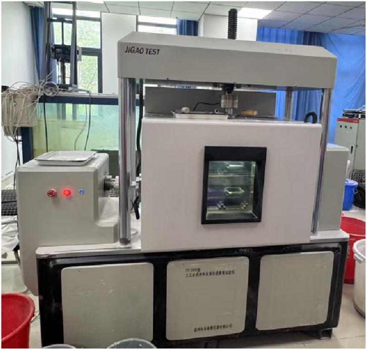
Large temperature-controlled straight shear.
2.3 Experimental process
Calcareous sand-geogrid interface pullout tests are carried out in an independently designed temperature-controlled test setup, and to ensure the reliability and reproducibility of the test results, all the tests are conducted under constant controlled environment and loading conditions with the following steps: (1) Sieve the calcareous sand to control the particle size distribution curve of each group of specimens to maintain consistency in order to exclude the influence of particle composition on the interfacial properties. Each group of specimens is filled into the draw box in three layers, and each layer was compacted in a standard way after filling to ensure the uniformity of specimen compactness and reduce the test error caused by uneven compaction. (2) In order to reduce the friction interference between the geogrid and the pulling box during the pulling process, petroleum jelly is uniformly applied to the opening of the inlet grating on the left side of the pulling box. After completing the first layer of specimen filling and compaction, the pre-cut geogrid is inserted through the opening and connected to the metal fixture connected to the horizontal force transducer, and the fixture bolts are subsequently tightened to secure the position of the geogrid. After completing the installation of the grids, the filling and compaction of the second and third layers of samples continued. In order to ensure comparability between samples of different particle sizes, the filling quality of each group of samples is controlled consistently, as shown in Table 3. After the filling, the top of the specimen is leveled, the loading steel plate is installed, and normal stress is administered through a bar controlled by a computer system. (3) Start the ambient temperature control system, set the target temperature value, and allow the specimen to stabilize consolidation at that temperature for 2 h to ensure that both the internal and external temperatures of the specimen reach the predetermined level. After the end of consolidation, the data acquisition system is zeroed. The test is conducted at a constant loading rate of 1 mm/min. The normal stresses are set at 20 kPa, 35 kPa and 50 kPa, and the test temperatures are set at 0 °C, 20 °C, 40 °C, 60 °C and 80 °C, forming 15 temperature-stress combinations to perform the pullout test in sequence.
TABLE 3
| Particle size (mm) | Calcareous sand quality (kg) | Normal stress (kPa) | Experimental temperature (°C) |
|---|---|---|---|
| S1 | 34.8 | 20, 35, 50 | −5, 0, 20, 40, 60, 80 |
| S2 | 30.9 | 20, 35, 50 | −5, 0, 20, 40, 60, 80 |
| S3 | 28.9 | 20, 35, 50 | −5, 0, 20, 40, 60, 80 |
Summary table of different specimen sands and test conditions.
3 Machine learning and deep learning algorithms
In this paper, four modeling methods are constructed, which cover three traditional machine learning models and one deep learning model, namely, SVM, PSO-SVM, GA-SVM, and LSTM. SVM, as an effective nonlinear regression method, exhibits strong modeling ability in small-sample, high-dimensional engineering problems. However, its performance depends on the reasonable setting of hyperparameters (e.g., penalty factor and kernel function parameters). To strengthen the generalization capacity and prediction precision of the model, this paper adopts two intelligent optimization algorithms, PSO and GA, respectively, to optimize the parameters of SVM, forming two integrated models, PSO-SVM and GA-SVM. In addition, this paper introduces the LSTM model with a time memory mechanism to better capture the dynamic evolutionary relationship between variables. The following subsections introduce the basic principles and implementations of the above four models in detail.
3.1 SVM
SVM is a supervised learning technique widely utilized for addressing both classification and regression problems. In regression problems, the goal of an SVM is to find a function such that the error between its predicted and actual values does not exceed a given tolerance ϵ, while maintaining the simplicity of the model. SVM are trained by constructing hyperplanes with a maximum interval in the feature space. To deal with nonlinearities, SVM employs a kernel function to project the input data into a high-dimensional feature space, where it determines the optimal regression function.
Equation 1 objective optimization problem of SVM regression model can be expressed as:where is the weight vector of the model, is the slack variable and C is a regularization parameter to balance the training error and model complexity.
Equation 2 for the constraints are:where is the target value, is the input data after mapping through the kernel function, is the weight vector of the model, is the tolerated error of the regression, and is the slack variable that allows some of the error to exceed the threshold.
Equation 3 for the final regression function is:
Where denotes the kernel function, and are the optimization variables obtained by the Lagrange multiplier method that determines the support vector. With these formulas, SVM can efficiently find the optimal solution in the regression problem.
3.2 PSO-SVM
PSO-SVM is a hybrid intelligent modeling method that combines particle swarm optimization algorithm and support vector machine. Its core idea is to use the global optimization capability of PSO to automatically find the optimal combination of key hyperparameters (including the regularization parameter C and the kernel function’s γ value) in SVM, thereby enhancing predictive performance and generalization. The performance of conventional SVM models is highly dependent on parameter selection, and inappropriate settings may lead to underfitting or overfitting. In contrast, PSO, as a heuristic optimization algorithm, which is a method that uses approximate search strategies to find near-optimal solutions, is based on population search and can perform efficient global search in the parameter space. Thus, it overcomes the limitations faced by traditional empirical settings or lattice searches. The modeling process of PSO-SVM consists of the following steps: firstly, initialize the particle swarm population, with each particle representing a possible (C, γ) parameter combination; secondly, evaluate each particle by a fitness function (e.g., the Cross-validation error) to evaluate the performance of each particle; then iteratively update the positions and velocities of the particles to continuously approximate the global optimal solution; finally, the optimal parameters are used to train the SVM model.
Equation 4 for the velocity and position update equations for the PSO are as follows:
Where and are the velocity and position of the and particle at the iteration, respectively; 3 and 4 are the historical optimal position and global optimal position of the particle, respectively; 6 is the inertia weight, 5 and 6 are the learning factors, and 7 and 8 are random numbers obeying [0,1]. Through the automatic optimization of SVM hyperparameters, PSO-SVM combines modeling accuracy and efficient parameter selection, and is applied to the task of predictive modeling of complex nonlinear problems.
3.3 GA-SVM
GA-SVM is a hybrid optimization model combining genetic algorithm and support vector machine, which aims to improve the prediction performance of the model by automatically optimizing the key hyper-parameters of the SVM through an intelligent search mechanism. SVM is effective for nonlinear, small-sample, and high-dimensional problems, but its predictive accuracy and generalization ability rely heavily on appropriate parameter settings. In GA-SVM, the prediction error on the training set serves as the fitness function. The algorithm starts by randomly initializing a population of chromosomes, each encoding a (C,γ) parameter pair. During each generation, selection, crossover, and mutation operations are performed to generate new solutions based on individuals with higher fitness, continuously improving the population quality. This iterative process continues until the maximum number of generations or a convergence criterion is reached. The final output is the optimal parameter set, which is then used to train the SVM model and achieve reliable predictive performance.
Equation 5 for the model optimization objective can be expressed as:where is the SVM prediction function for the given parameters and is the true value.
3.4 LSTM
Long Short-Term Memory Networks (LSTM), a widely adopted variant of Recurrent Neural Networks (RNN), have been shown to be very effective in modeling time series data and capturing long-range dependencies. LSTM is first proposed by Sepp Hochreiter and Jürgen Schmidhuber in 1997 to solve the problem of gradient vanishing, which is commonly encountered in traditional RNN. The LSTM cell consists of three main components: an input gate, a forgetting gate, and an output gate. These gates collaborate to regulate the input, output, and cell state of the information flow, and the cell state is the memory component of the network.
Equations 6–11 for the working principle of LSTM unit can be represented by the following mathematical expression:where denotes the input of the time step, is the hidden state of the previous moment, is the RELU activation function, is the hyperbolic tangent function, the symbol *denotes the element-by-element multiplication operation, are the weight matrices corresponding to the gating structure, and are the bias vectors, respectively. These parameters are optimized by backpropagation during the training process. The final output hidden state can be used in the subsequent fully connected layer for regression analysis or passed to the next LSTM unit. Due to its gating mechanism that can stably control the gradient flow, LSTM shows good robustness in handling nonlinear and non-smooth time series data. Therefore, it is used in this paper for the task of modeling time-varying shear strength prediction. The structure of the LSTM model is shown in Figure 3.
FIGURE 3

Schematic diagram of LSTM structure.
4 Methodology
4.1 Data collection and preprocessing
Based on the experimental data, a database including 1178 data points was developed. The data are randomly divided into 943 training data sets (80%) for training the machine learning models and 235 test data sets (20%) for testing the constructed machine learning models. Deep learning, on the other hand, randomly divides the data into 825 training data sets (70%), 235 test data sets (20%), and 118 validation data sets (10%). For each data set, grain size, temperature, normal displacement and shear displacement are used as input parameters, and the shear strength of calcareous sand-geogrid is used as the output parameter. Figure 4 shows how the input parameters are distributed in the constructed database, with the x-axis indicating parameter values and the y-axis showing the frequency of their occurrence. The correlation between variables is analyzed using Pearson’s correlation coefficient, and the results are shown in Figure 5. In summary, the data from this experiment are suitable for artificial intelligence modelling in terms of sample size, variable distribution, and independence between variables.
FIGURE 4
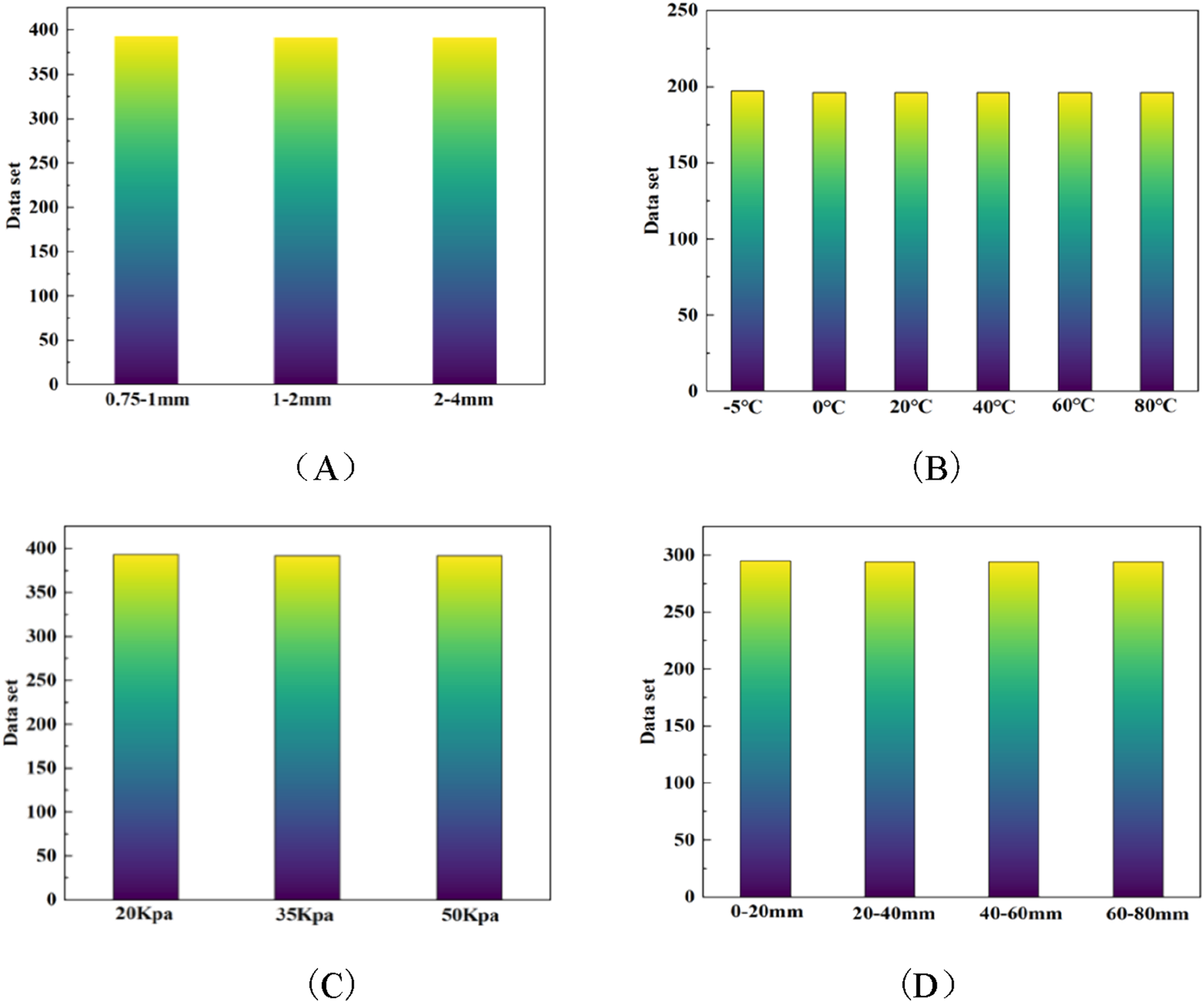
Distribution of data sets. (A) Particle size. (B) Temperature. (C) Normal stress. (D) Shear displacement.
FIGURE 5
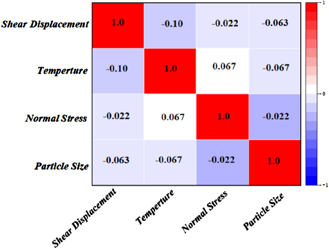
Correlation matrix map of the input features.
In the research, before conducting machine learning and deep learning modelling. It is necessary to standardize various dimensions of the input and output variables to enhance the predetermined accuracy and efficacy of the machine learning algorithm and express Equation 12 for normalization, and Equations 13–16 are also included.
Where x is the original data value, is the normalized data value, xmin is the smallest value in the data, and xmax is the largest value in the data set.
4.2 Performance evaluating approaches
To comprehensively evaluate the predictive performance of the constructed model, this study selects the RMSE , MAPE, MAE, MSE are evaluation indicators. These indicators can comprehensively evaluate the model from multiple dimensions, such as error size, relative error, model stability and outlier sensitivity, and comprehensively analyze the accuracy and robustness of the model.
1. RMSE is a commonly used indicator to measure the degree of error fluctuation between the predicted value and the actual value, and its calculation formula is shown in (13), which can reflect the standard deviation of the model’s predicted value. It can reflect the standard deviation of the predicted values of the model, and the smaller the RMSE value, the lower the overall prediction error of the model and the better the fitting effect.
2. MAPE is a relative error metric that measures the average percentage deviation of the predicted values from the actual values, and its calculation formula is shown in (14). Unlike RMSE, MAPE standardizes the error and is suitable for comparing prediction models with different data sizes. The smaller the MAPE value, the lower the average relative error of the model.
3. MAE is used to measure the average absolute deviation between the predicted value and the actual value, and its calculation formula is shown in (15). This indicator gives the same weight to all errors, which can intuitively reflect the average prediction deviation of the model. The smaller the MAE value, the better the overall prediction effect of the model.
4. MSE is an important measure of the squared average of the prediction error, and its calculation formula is shown in (16). Unlike RMSE, MSE retains the form of error squared, which gives it a higher penalty for large errors and helps the model focus more on the optimization of extreme prediction errors. A lower MSE indicates greater model accuracy and reduced prediction error.
where
nis the total number of samples,
yirepresents the
iobserved value, and
firepresents the
ipredicted value. The three remaining formulas are identical.
4.3 Hyperparameter optimization
4.3.1 Hyperparameter optimization of GA and PSO
To optimize the Support Vector Machine (SVM) model parameters C and g, this study employs two evolutionary algorithms—GA and PSO. Table 4 summarizes the detailed configuration of hyperparameters for both algorithms. In the GA-SVM model, the population size is set to 20 and the number of generations to 200. The selection operation uses the normalized geometric selection method with a selection pressure parameter of 0.09. The algorithm applies arithmetic crossover with a crossover probability of 0.9 and performs mutation using a non-uniform mutation strategy. The search range for both c and g is set to [0.1, 100], and the termination condition for evolution is defined as an optimal solution tolerance threshold of 200 generations. The fitness function is calculated based on cross-validation accuracy to ensure generalization performance.
TABLE 4
| Hyperparameters | Parameter name | Range of values |
|---|---|---|
| GA | Population size (pop_num) | 20 |
| Number of Generations (maxgen) | 200 | |
| Selection function parameter (normGeomSelect) | 0.09 | |
| Crossover function parameter (arithXover) | 0.9 | |
| Parameter Range | Both C and g are within [0.1, 100] | |
| Optimal solution tolerance (maxGenTerm) | 200 | |
| Fitness Function | Cross-Validation | |
| PSO | Learning factors (c1, c2) | C1 = 1.5,C2 = 1.7 |
| Maximum position (popmax) | Cmax = 100; gmax = 1e-3 | |
| Minimum position (popmin) | Cmax = 0.1; gmax = 1e-3 | |
| Population size (sizepop) | 10 | |
| Population update times (maxgen) | 100 | |
| Training Epochs | k-Fold Cross-Validation | |
| Training iterations (epochs) | 100 |
Parameter settings for GA and PSO optimized SVM.
In the PSO-SVM model, the learning factors are set to c1 = 1.5 and c2 = 1.7, balancing the global and local search abilities. The position ranges for C and g are defined as [0.1, 100] and [10–3, 1], respectively. The swarm size is 10, and the optimization process runs for 100 generations. Model training incorporates 5-fold cross-validation to evaluate fitness, and each candidate SVM is trained for 100 epochs to ensure convergence.
4.3.2 LSTM parameter settings
In this study, the LSTM model is employed to capture the temporal dependencies of the input features. The hyperparameter configuration is summarized in Table 5. The architecture consists of two LSTM layers: the first layer has 64 units and returns sequences for the second layer, which contains 32 units. A fully connected (d4ense) layer with 50 neurons follows, and a final dense output layer performs regression prediction.
TABLE 5
| Layer type | Parameter name | Value |
|---|---|---|
| Input Layer | Input Shape | (300, 4) |
| LSTM Layer 1 | Number of Units | 64 |
| Return Sequences | True | |
| LSTM Layer 2 | Number of Units | 32 |
| Return Sequences | False (default) | |
| Fully Connected | Number of Neurons | 50 |
| Activation Function | ReLU | |
| Training Settings | Batch Size | 32 |
| Epochs | 50 | |
| Validation Split | 0.1 | |
| Time Step Length | time_steps | 300 |
| Optimization | Optimizer | Adam |
Parameter settings of LSTM.
To balance computational efficiency and model performance, a combination of trial-and-error and random search is used for hyperparameter tuning. The optimized hyperparameters include the time step size (set to 300), the number of LSTM units, the number of neurons in the dense layer, the number of training epochs (50), batch size (32), and the activation function (ReLU). To optimize the model, the Adam algorithm is applied in conjunction with the mean squared error loss function. During training, 90% of the training data is used for model fitting, and 10% is reserved for validation to ensure generalization performance.
As shown in Figure 6, the loss function of the LSTM model during training and validation shows an overall decreasing trend as the number of training rounds increases. The training loss (blue solid line) and validation loss (orange dashed line) decrease rapidly in the initial phase, which indicates that the model quickly learns the basic patterns in the training data in the initial phase. As can be seen in Figure 6, the loss values of the LSTM model decrease rapidly within the first 10 training rounds, which indicates that the model has effectively learned the main features in the input data in the early stage. As the number of training rounds increases, the rate of loss decline gradually slows down and stabilizes after about the 35th round, which indicates that the model has basically completed the learning of the relationship between the input features and the output target and enters the convergence state. Overall, the gap between the training loss and the validation loss is always small, and both tend to be smooth at the same time, which indicates that the LSTM model maintains strong consistency and stability during the training process and does not have obvious overfitting or underfitting phenomena.
FIGURE 6
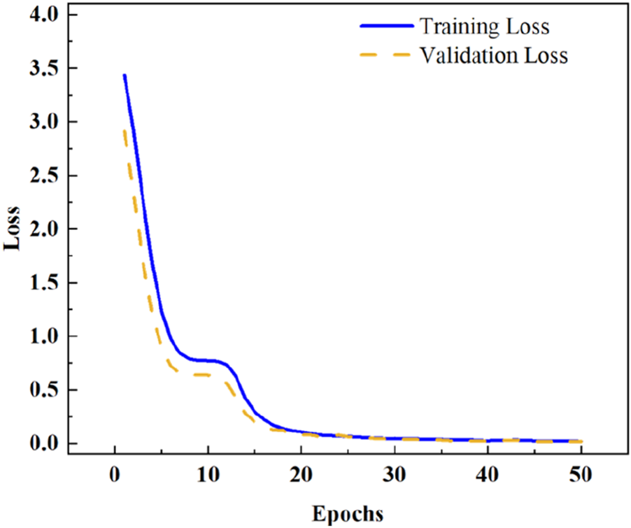
The loss function curve of deep learning LSTM models.
5 Results and analysis
5.1 Model training and testing
To assess the predictive performance of various models for the peak shear strength of CSGI, this study trains four models: SVM, PSO-SVM, GA-SVM, and LSTM. The prediction effects are visualized and compared on the training set, and the results are shown in Figure 7.
FIGURE 7
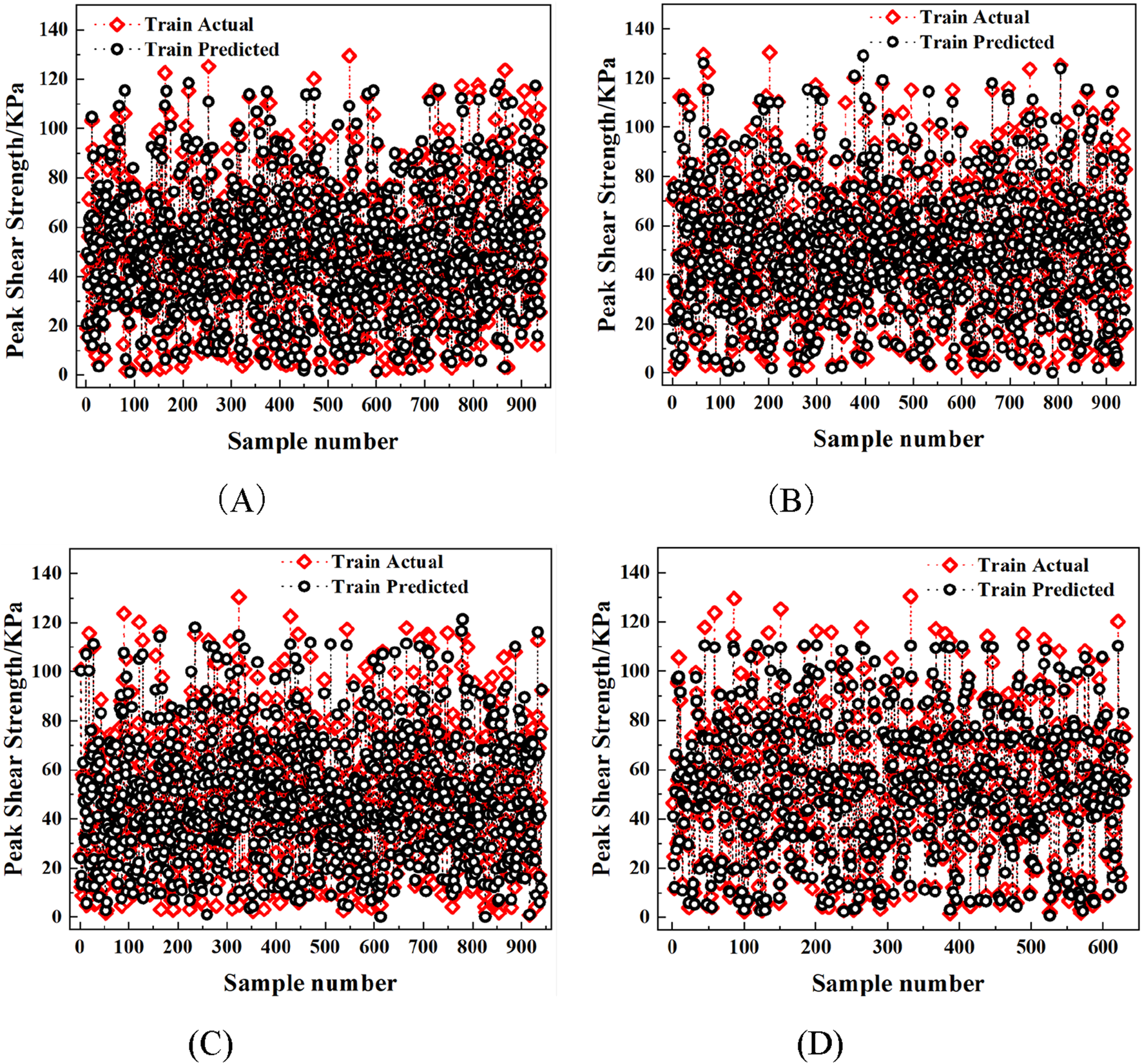
Prediction results of training set on test data. (A) SVM. (B) PSO-SVM. (C) GA-SVM. (D) LSTM.
A visual comparison of machine learning models and deep learning models on the test set is shown in Figure 8 below.
FIGURE 8
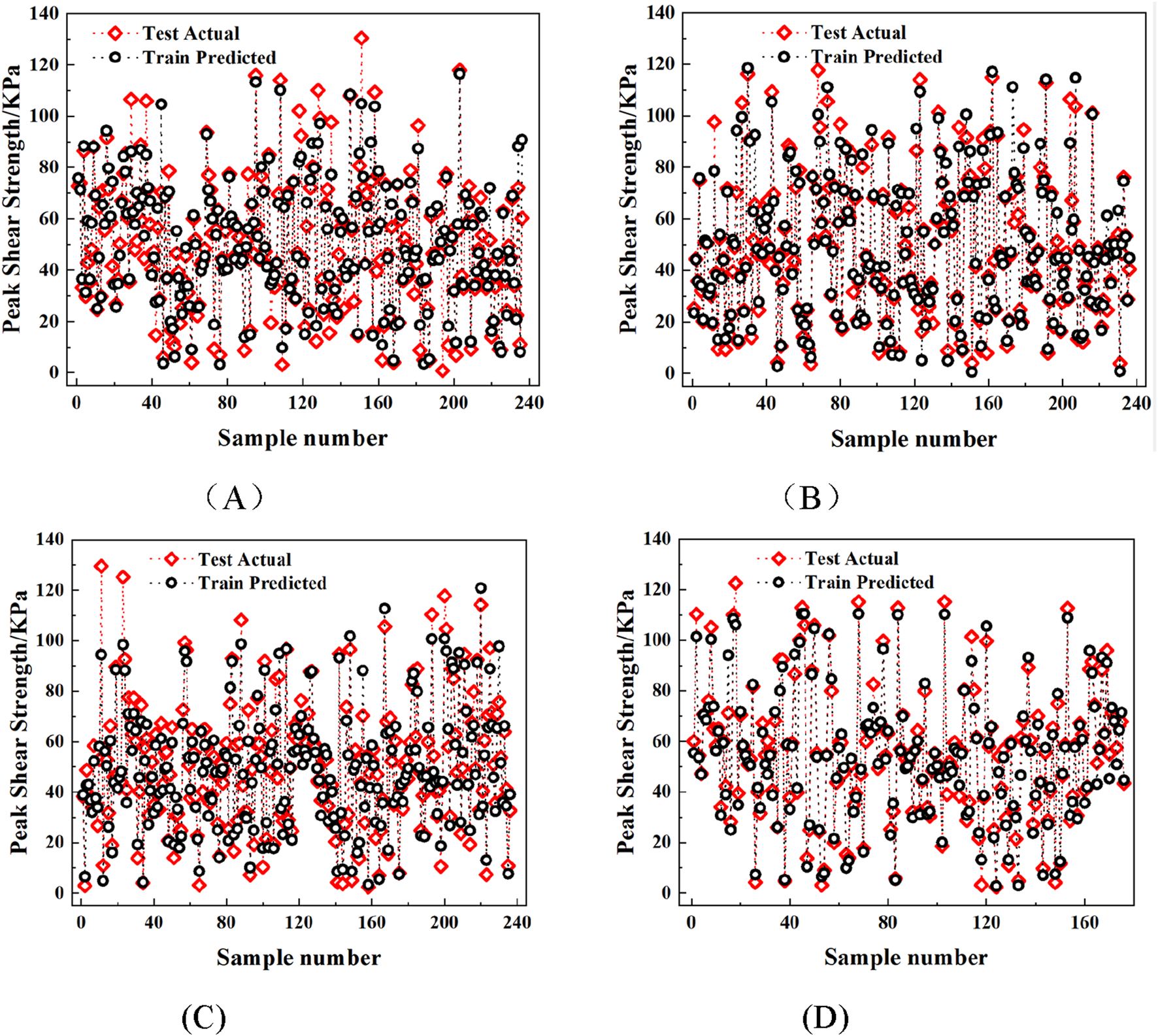
Prediction results of test set on test data. (A) SVM. (B) PSO-SVM. (C) GA-SVM. (D) LSTM.
Figures 7, 8 show the prediction results of the SVM, PSO-SVM, and GA-SVM models. The predicted values (red hollow circles) and actual values (black solid circles) exhibit a high degree of agreement. This indicates that all models capture the main trends of the dataset. The SVM model performs relatively uniformly across the dataset. However, it presents fluctuations in larger value intervals. The PSO-SVM model achieves higher stability and accuracy by introducing particle swarm optimization. The GA-SVM model further improves the point cloud distribution. Red points are closely concentrated near the black points. This demonstrates the advantage of the genetic algorithm in global search and its contribution to overall prediction performance. Overall, these results indicate that optimization algorithms enhance the predictive capability of SVM models. They provide more reliable guidance for interface mechanical property prediction under varying conditions. Compared with the traditional machine learning model, the LSTM model has a significant advantage in processing time series data, and its prediction results have the highest degree of agreement with the actual values. The overlap between the red and black points in Figure (D) is significantly higher than that of the other three models, indicating that LSTM is better able to capture the complex nonlinear relationship between the input variables and the output. Overall, the LSTM model has the best prediction on the training set, followed by GA-SVM and PSO-SVM, while the traditional SVM model has relatively weak performance in this study.
5.2 Model comparisons
Visualization comparison plots of machine learning models and deep learning models in terms of R2 values have been created on the training dataset and test dataset, as shown in Figures 9, 10.
FIGURE 9
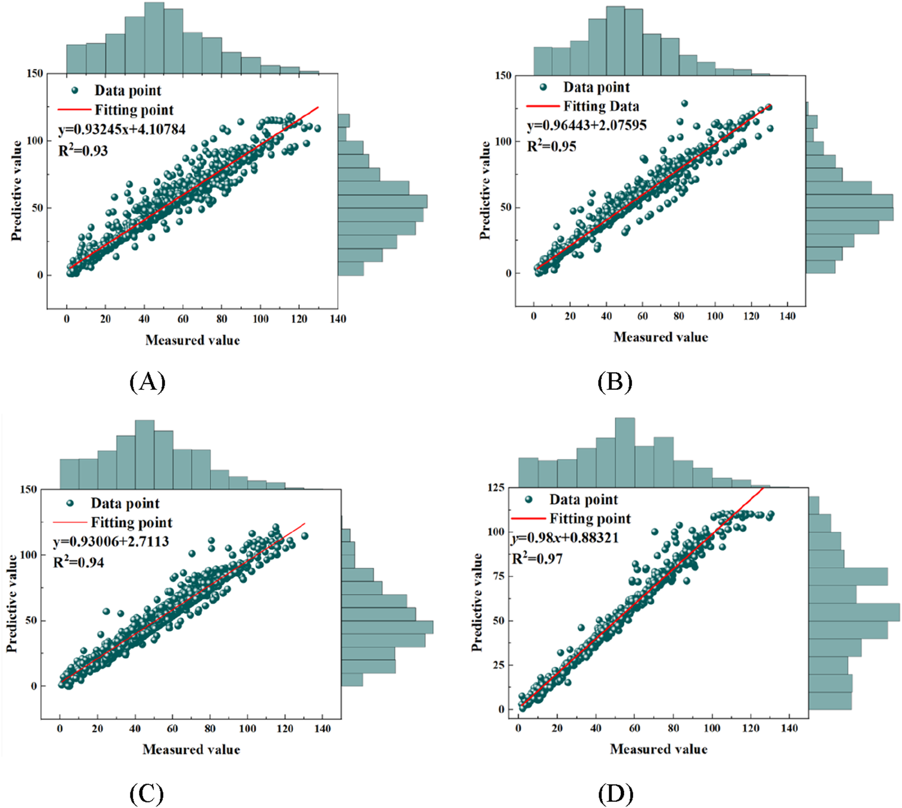
The R2 value of the training dataset. (A) SVM. (B) PSO-SVM. (C) GA-SVM. (D) LSTM.
FIGURE 10
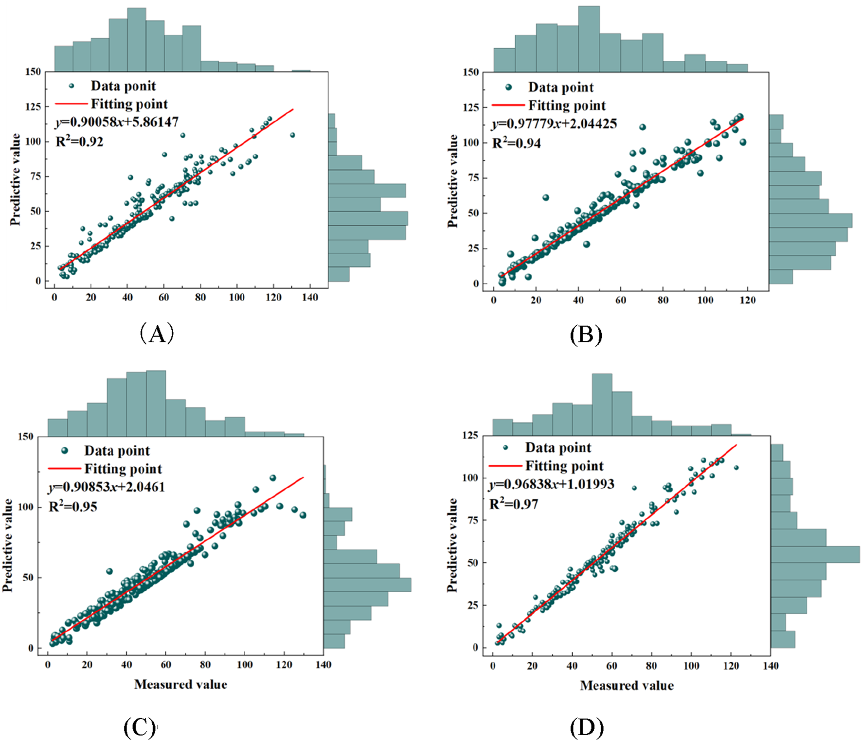
R2 value of the test data set. (A) SVM. (B) PSO-SVM. (C) GA-SVM. (D) LSTM.
Figure 10 illustrates the regression relationship between predicted and actual values for various models on both training and testing datasets. The green scatters indicate the data points of the model predicted values and the corresponding measured values, and the red straight line is the linear fitting result. The green scatters in the image indicate the data points corresponding to the predicted and measured values of the model, and the red straight line is the result of the optimal linear fit. The fitting equation and the coefficient of determination, R2, are used to quantify the fitting accuracy of the model. The edge histograms of predicted and measured values are also plotted on both sides of the image to assist in judging the distribution characteristics and consistency of the data. From the overall results, all the models show strong regression ability in the training and testing stages, with regression slopes close to 1, small intercepts, and decision coefficients R2 higher than 0.92, which indicate that the models have good explanatory and generalization performance in predicting the interfacial shear strength. Specifically, the SVM model performs in the training set Figure 9A with the fitted equation y = 0.93245x+4.0784 and R2 = 0.93, which shows a better regression. The R2 = 0.92 in the test set Figure 10A indicates that there is some difference in the generalization ability of the model. Especially in the high value band where there is a slight tendency for underestimation. The performance of the PSO-SVM model is further improved, with the R2 = 0.95 in the training set Figure 9B, the fitting slope is significantly close to 1, the error fluctuation is reduced, and it shows a good middle and high value fitting ability. The R2 = 0.94 in the test set Figure 10B indicates that the model still maintains a high level of prediction accuracy on unseen data and shows superior robustness. The GA-SVM model has R2 = 0.94 in the training set Figure 9C and R2 = 0.95 in the test set Figure 10C, which shows a high generalization ability, but the model may still have a slight bias in the low-value band. In contrast, the LSTM model performs best. The R2 = 0.97 in Figure 9D of the training set, the regression slope is extremely close to 1, and the intercept is close to 0, which indicates that the model prediction almost reaches the ideal linear state. The error distribution is uniform and there is no obvious systematic bias. In Figure 10D of the testing set, the R2 = 0.97 has a high goodness-of-fit, which indicates that it has a good prediction accuracy over the whole range. Especially when dealing with the complex nonlinear time series problem, the LSTM model shows stronger learning and generalization ability.
Overall, although all models have good prediction performance, they differ in terms of accuracy and stability. The traditional SVM model is relatively weak in fitting ability, and optimization algorithms such as PSO and GA improve the model performance to a certain extent, among which the SVM under PSO optimization has the strongest fitting consistency in the training and testing phases. The deep learning model LSTM, on the other hand, with its structural advantages, not only has the highest fit on the training set but also shows great accuracy and robustness in the testing phase.
5.3 Evaluation index assessment
The prediction performance of four models, SVM, PSO-SVM, GA-SVM and LSTM, is systematically evaluated and comparatively analyzed using four key evaluation indexes, namely, RMSE, MAPE, MAE and MSE, and the specific results are shown in Figure 11.
FIGURE 11

RMSE, MAPE, MAE, MSE evaluation indicators. (A) RMSE. (B) MAPE. (C) MAE. (D) MSE.
Figures (A) to (D) illustrate the predictive performance of various models on both the training and test sets, evaluated using RMSE, MAPE, MAE, and MSE. The results show that the LSTM model exhibits optimal performance in all evaluations. The RMSE, MAPE, MAE and MSE on the training set are 4.32, 8.18%, 2.74 and 18.64, respectively, while the corresponding values on the test set are 4.35, 9.51%, 3.00 and 18.95. All four indicators are the lowest. Moreover, the performance gap between training and testing is extremely small, demonstrating its outstanding fitting ability and generalization ability. Secondly, the SVM model is optimized by PSO. The RMSE, MAPE, MAE and MSE on its training set are 5.64, 9.96%, 3.07 and 31.76, respectively, while those on the test set are 6.30, 10.67%, 3.37 and 39.70 respectively. Each index is slightly higher than that of LSTM but significantly better than other SVM models. The metrics of the SVM model optimized by GA on the training set are 6.17 (RMSE), 12.56% (MAPE), 4.13 (MAE), and 38.09 (MSE), and those on the test set are 6.26, 13.00%, 4.23, and 39.23, indicating that although its optimization effect is better than that of the traditional SVM, it is not as good as that of PSO optimization. The traditional SVM model performs the worst in all four indicators, with the training set errors being 6.92 (RMSE), 13.8% (MAPE), 4.27 (MAE), and 47.82 (MSE), respectively. The test set is even higher, 7.77, 15.38%, 4.75, and 60.39 respectively, demonstrating weak fitting ability and overfitting risk.
Overall, the deep learning-based LSTM model is optimal in all four error evaluation metrics and exhibits the smallest error and strongest generalization ability in both the training and testing phases, which significantly outperforms the traditional SVM as well as the GA and PSO-optimized SVM. The PSO-SVM model is ranked the second best among all the SVM family of models, which indicates that the PSO algorithm is more effective than the GA algorithm in parameter finding and optimization. In contrast, GA optimization has limited improvement in SVM performance, while the unoptimized SVM model has the worst prediction accuracy and suffers from underfitting and insufficient generalization ability. In terms of overall performance, the LSTM model is the algorithmic tool with the best prediction performance in the context of the current problem. Especially for dealing with highly nonlinear and complex datasets, and significantly outperforms traditional machine learning methods based on support vector machines in terms of fitting accuracy and stability.
5.4 SHAP sensitivity analysis
SHapley Additive exPlanations (SHAP) is an interpretability method grounded in game theory that measures the contribution of each feature to the output of a single model prediction. Thus revealing the “black box” mechanism inside deep learning models, which is proposed by Scott Lundberg and Su-In Lee (Lundberg and Lee, 2017) in 2017. In order to further explain the prediction logic of the LSTM model and enhance the credibility of the model in geotechnical engineering applications, this paper adopts the SHAP method to perform a sensitivity analysis on the input features of the model. The value quantifies the contribution of each feature to the model output and is ranked in descending order of importance. A positive SHAP value indicates that the feature has an increasing effect on the prediction, while a negative SHAP value indicates a decreasing effect. Equation 17 for the mathematical framework, and Equations 18–23 are also included.
Figure 12 illustrates the results of the feature importance analysis, including a bar chart of the global average SHAP values and a swarm summary chart.
FIGURE 12
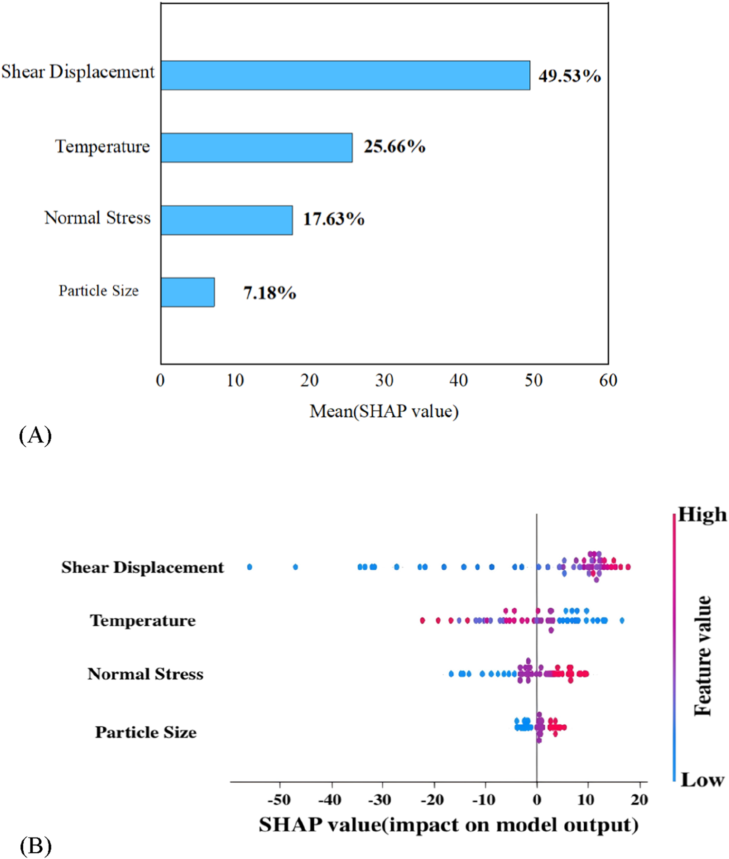
Feature Importance Analysis Diagram. (A) Global bar chart based on SHAP values. (B) Beeswarm summary plot based on SHAP values.
As shown in Figure 12A, the horizontal axis represents the average SHAP value of each input variable, which represents its average contribution to the predicted output of the model. The features are ranked in order of influence from top to bottom. According to the results of the Figure 12A, “shear displacement” is the most influential variable in the model, with an average SHAP value of 49.53%, indicating that this variable plays a dominant role in the prediction of the peak shear strength of the interface. It is followed by “temperature” at 25.66%, “normal stress” at 17.63% and “particle size” at 7.18%.
Figure 12B further demonstrates the specific trends of the influence of each variable on the model output through a swarm summary plot. The horizontal axis is the SHAP value, the vertical axis is the name of the variable, and the colour of the dots represents the high or low value of the variable (red is high, blue is low). As can be seen from the Figure 12B, for “shear displacement”, the SHAP values corresponding to the high value samples are mostly positive. This indicates that when this variable is large, it has a significant positive driving effect on the model predicted output. In other words, the larger the shear displacement is, the easier it is for the interface to reach a higher shear strength. A similar trend is observed for “temperature”. Most of the sample points under high temperature conditions are located in the positive SHAP region, suggesting that higher temperatures contribute to higher interfacial strengths. This is due to the friction-enhancing effect of material softening at high temperatures. In contrast, the distribution of SHAP values for “normal stress” is more discrete, containing both positive and negative values, indicating that its effect is regulated by the shear displacement path and the interface state, and it may be enhanced or weakened under different working conditions. The overall effect of “particle size” on the model is small, which reflects that its contribution to the shear strength is small in the range of data studied.
6 Empirical formula
This study shows that the LSTM model exhibits high accuracy and good stability in predicting the shear strength of the CSGI and is able to effectively capture the complex nonlinear relationship between the input parameters and the mechanical response of the interface. Although the deep learning model has significant advantages in dealing with unstructured data and nonlinear problems, and it has no obvious defects in its generalization ability and expression ability, for engineers and technicians who lack relevant background knowledge, the direct application of this kind of “black-box” model is still a big obstacle to meet the requirements of engineering practice for simplicity and operability. However, for engineers and technicians without relevant background knowledge, there is still a big obstacle to the direct application of these “black box” models. It is difficult to meet the demand for simplicity and operability in engineering practice. Therefore, drawing on P. Debnath’s research idea, a systematic analysis of the model prediction results is conducted by combining the input parameters temperature (T), particle size (P), normal stress (N), and shear displacement (S). The reference values for these parameters are chosen close to their mean values, as shown in Table 6. SHAP is then used to perform a sensitivity analysis of the model. The results indicate that shear displacement has the greatest impact on shear strength. To further assess the effect of each input parameter on the shear strength prediction, one parameter is varied at a time while keeping the others fixed at their reference values, and fitting analysis is performed. The correction factors used to improve the shear strength prediction accuracy are derived through a fitting process. This process involves adjusting the model parameters to minimize the error between the predicted shear strength and the experimental results. During this procedure, different correction factor values are iteratively tested, and the model’s performance is assessed using error metrics such as the root mean square error (RMSE) or the coefficient of determination (R2). The optimal correction factors are identified through this iterative process, which enhances the overall predictive accuracy of the empirical formula.
TABLE 6
| Statistical index | Particle size (mm) | Temperature (°C) | Normal stress (kPa) | Shear displacement (mm) |
|---|---|---|---|---|
| Mean | 0.837209 | 27.47508 | 34.65116 | 21.71493 |
| Referece | 0.84 | 28 | 35 | 22 |
Reference values for input parameters.
An empirical model for predicting interface shear strength is developed by considering the relationship between each input parameter and shear strength. Interpretation of the characteristic importance of the model outputs through the SHAP method shows that shear displacement (S) is the most sensitive parameter that has the greatest influence on the shear strength. As shown in Figure 11, the prediction results of the variation of shear strength (qs) with shear displacement (S) are shown under the condition that the other input parameters take the reference values.
Final empirical equations for the relationship between the shear strength qss at the calcareous sand-geogrid interface and key input parameters (18):
Figure 13 shows that shear displacement (S) is the most sensitive parameter in the process of predicting the shear strength qss. In order to fully consider the effects of other input parameters on qss prediction, an empirical prediction equation including the correction function F is constructed as shown in Equation 19:
FIGURE 13
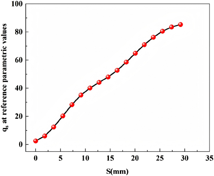
LSTM prediction of qs with reference parameter value S.
The correction function F is used to reflect the correction effect of particle size (P), temperature (T), normal stress (N) and other influencing factors on the prediction of shear strength, the specific expression is shown in Equation 20:
Using the method proposed by P. Debnath (Debnath and Dey, 2018), the expressions for each correction factor are obtained by fitting the experimental data to the model predictions, as shown in Equation 21 through (23):
C P is the correction factor for particle size, CT is the correction factor for temperature, and CN is the correction factor for normal stress.
7 Experimental verification
In order to verify the applicability of the LSTM and empirical formulae models, the empirical formulae are therefore applied to predict the shear strength of the CSGI under different temperature conditions and compared with the experimental results. As shown in Table 7, 27 sets of tests are randomly selected from the experimental data. According to the experimental conditions and requirements, Equation 18 is used to estimate the predicted shear strength of calcareous sand-geogrid interfaces with different particle size gradations under various conditions. The predicted shear strengths are compared with the shear strengths of existing studies, as shown in Figure 14.
TABLE 7
| Particle size (mm) | Temperature (°C) | Normal stress (kPa) | Shear displacement (mm) | Shear stress (kPa) |
|---|---|---|---|---|
| S1 | −5 | 20 | 2.0248 | 8.49285 |
| −5 | 20 | 4.0123 | 12.44025 | |
| −5 | 20 | 6.0091 | 15.90915 | |
| S1 | 40 | 20 | 18.018 | 31.33985 |
| 40 | 20 | 22.0085 | 33.7322 | |
| 40 | 20 | 26.0208 | 35.1676 | |
| S1 | 60 | 20 | 4.0123 | 13.5168 |
| 60 | 20 | 6.006 | 17.16515 | |
| 60 | 20 | 8.0028 | 20.2752 | |
| S2 | −5 | 35 | 6.0091 | 39.47385 |
| −5 | 35 | 8.0246 | 50.53845 | |
| −5 | 35 | 10.0183 | 60.40695 | |
| S2 | 0 | 35 | 2.0123 | 12.44025 |
| 0 | 35 | 4.006 | 24.8805 | |
| 0 | 35 | 6.0247 | 35.7657 | |
| S2 | 80 | 35 | 2.0186 | 10.2871 |
| 80 | 35 | 4.0123 | 16.56705 | |
| 80 | 35 | 6.006 | 21.7106 | |
| S3 | −5 | 20 | 1.0217 | 7.11725 |
| −5 | 20 | 2.0186 | 12.2608 | |
| −5 | 20 | 4.0123 | 23.26565 | |
| S3 | 20 | 35 | 2.0217 | 8.97135 |
| 20 | 35 | 4.0123 | 25.5982 | |
| 20 | 35 | 6.006 | 39.53365 | |
| S3 | 40 | 20 | 1.0217 | 3.11005 |
| 40 | 20 | 2.517 | 6.6986 | |
| 40 | 20 | 4.0154 | 12.1412 |
27 data sets selected for the test.
FIGURE 14
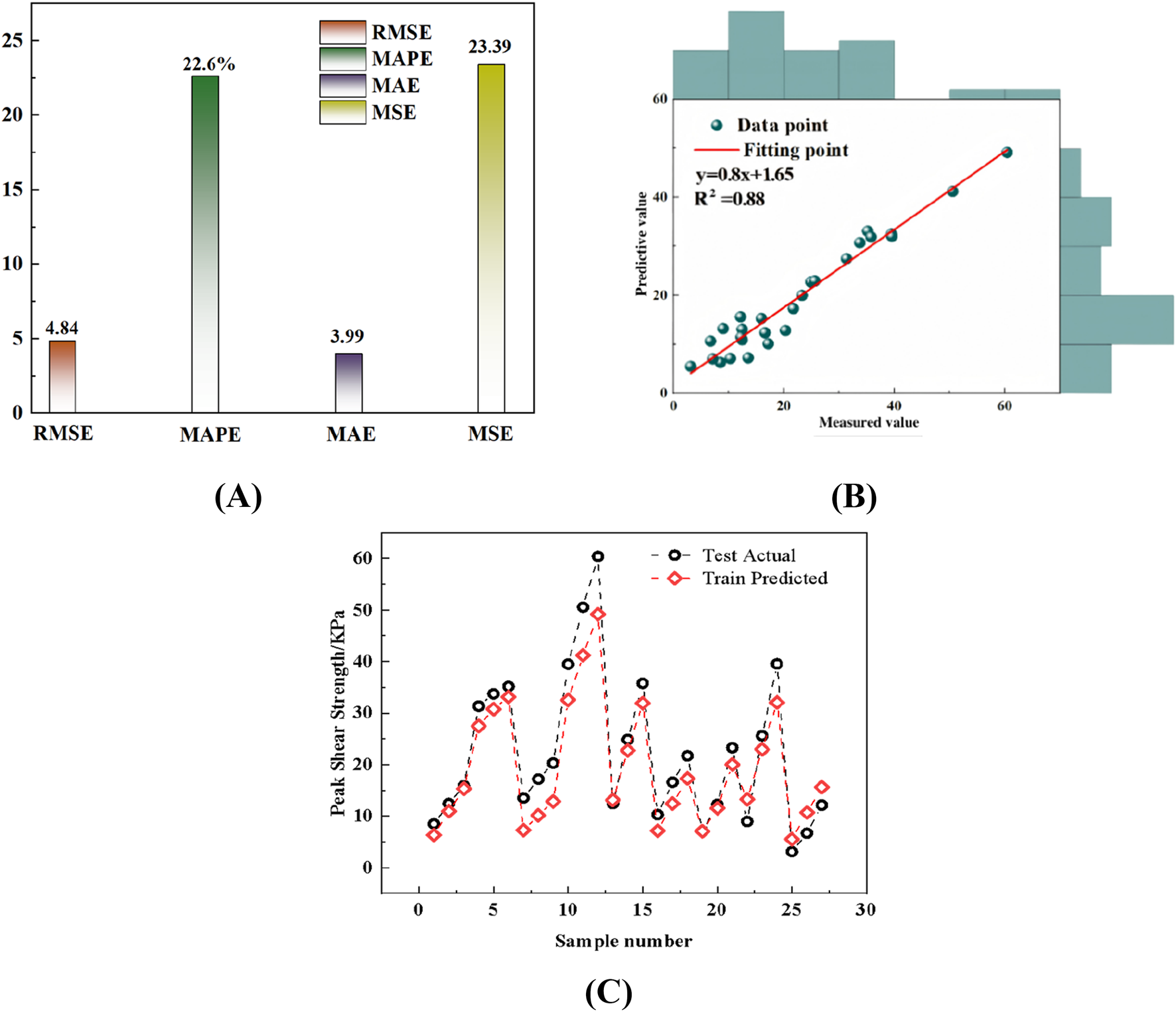
Performance evaluation of predicted shear strength of calcareous sand-geogrid interface based on empirical equations. (A) RMSE, MAPE, MAE and MSE values. (B) The value of R2.(C) Real and predicted values.
An empirical formula for shear strength prediction is constructed based on the LSTM model, and its prediction performance is evaluated. As can be seen in Figure 12, the empirical formula performs as follows in terms of prediction metrics:(A) In the Figure A, the RMSE is 4.84, the MAPE is 22.6%, the MAE is 3.99, and the MSE is 23.29. In the Figure (B), the coefficient of determination (R2) reaches 0.88. Although there is a gap in the prediction accuracy compared with the deep learning model (average R2 is above 0.95), the empirical formula has a certain gap in prediction accuracy, but its error range is still within the acceptable range and has good applicability and stability. It is worth noting that although the deep learning model can realize higher accuracy prediction, its deployment and use are often limited by strong data dependence, high requirement of computational resources, and poor interpretability during the promotion and application in the engineering field. In contrast, empirical formulas can provide low-threshold auxiliary decision-making means for field engineers due to their clear form, simple calculation, and easy integration into the conventional design calculation process.
To further assess the predictive performance and generalizability of the empirical model, eighteen data points are selected from the literature (Chao et al., 2024c) and are listed in Table 8. The selected data cover two particle size ranges (1–2 mm and 2–4 mm), temperatures ranging from −5 °C to 40 °C, and normal stresses of 15, 25, and 50 MPa. These combinations fall within the experimental range but represent different conditions from the original training dataset. As shown in Figure 15, the prediction results demonstrate good agreement with the literature values. The evaluation metrics and the correlation coefficient R2 = 0.82) indicate that the empirical model maintains reliable predictive capability across different particle sizes, temperatures, and stress levels.
TABLE 8
| Particle size (mm) | Temperature (°C) | Normal stress (kPa) | Shear displacement (mm) | Shear stress (Kpa) |
|---|---|---|---|---|
| S1 | −5 | 15 | 5.2583 | 9.8334 |
| −5 | 25 | 10.1678 | 18.1667 | |
| −5 | 50 | 10.2675 | 32.3335 | |
| S2 | −5 | 15 | 11.4886 | 10.2223 |
| −5 | 25 | 14.7128 | 16.1112 | |
| −5 | 50 | 19.264 | 28.5557 | |
| S1 | 20 | 15 | 9.613 | 12.444 |
| 20 | 25 | 14.454 | 15.445 | |
| 20 | 50 | 10.043 | 23.389 | |
| S2 | 20 | 15 | 10.962 | 11.556 |
| 20 | 25 | 16.355 | 15.833 | |
| 20 | 50 | 17.492 | 27.611 | |
| S1 | 40 | 15 | 10.791 | 10.944 |
| 40 | 25 | 14.784 | 16.278 | |
| 40 | 50 | 17.893 | 33.945 | |
| S2 | 40 | 15 | 17.943 | 10.5 |
| 40 | 25 | 14.928 | 14.945 | |
| 40 | 50 | 20.716 | 24.333 |
18 data sets selected for the test.
FIGURE 15

Empirical model generalizability evaluation. (A) RMSE, MAPE, MAE and MSE values. (B) The value of R2. (C) Real and predicted values.
8 Conclusion
In this study, pullout tests are conducted at the calcareous sand-geogrid interface under different temperatures and normal stress conditions. And a database containing 1178 sets of data is constructed. On this basis, four prediction models, including three traditional machine learning models (SVM, PSO-SVM, GA-SVM) and one deep learning model (LSTM), are established for predicting the shear strength of the CSGI. The models integrate key input variables such as temperature, particle size, normal stress and shear displacement, and the performance of each model is comprehensively compared and analyzed by error metrics with coefficients of determination. Meanwhile, the importance of model input parameters is quantitatively analyzed using the SHAP method, and an empirical formula for easy engineering application is constructed based on the deep learning results. The main research conclusions are as follows:
1. The study confirms that the shear strength of the CSGI is strongly influenced by elevated temperatures. This highlights the necessity of accounting for thermal coupling effects in foundation treatment and structural design within high-temperature marine environments.
2. Deep learning methods, particularly the LSTM model, demonstrate superior predictive accuracy and robustness compared with traditional machine learning approaches. This suggests that advanced artificial intelligence models can serve as reliable tools for predicting complex interfacial behaviors.
3. Sensitivity analysis reveals that shear displacement is the dominant factor affecting interfacial shear strength, followed by temperature, normal stress, and grain size. These insights provide guidance for prioritizing key parameters in engineering design and improving the efficiency of interface performance optimization.
4. The development of an empirical formula, derived from the LSTM model and SHAP analysis, bridges advanced artificial intelligence findings with practical engineering needs. This formula offers a balance between computational simplicity and predictive reliability. It is particularly valuable for field applications where deep learning resources are not available.
In contrast, the traditional machine learning models (SVM, PSO-SVM, GA-SVM) exhibited relatively lower prediction accuracy. This can be attributed to their limitations in capturing the complex, nonlinear relationships between input variables and shear strength. These limitations become more pronounced when the data is strongly influenced by environmental factors such as temperature. While these models perform well in simpler, more linear environments, they struggle to capture the intricate interactions between various parameters. In contrast, deep learning models, such as LSTM, excel at this task due to their ability to learn hierarchical patterns in data.
Overall, the prediction of shear strength at the calcareous sand-grid interface is affected by a combination of multiple complex nonlinear factors, which makes accurate modelling more challenging. The LSTM model In contrast, the traditional machine learning models (SVM, PSO-SVM, GA-SVM) exhibited relatively lower prediction accuracy. This can be attributed to their limitations in capturing the complex, nonlinear relationships between input variables and shear strength, especially when the data is highly influenced by environmental factors such as temperature. While these models perform well in simpler, more linear environments, they struggle to model the intricate interactions between the various parameters at play, which deep learning models, like LSTM, excel at due to their ability to learn hierarchical patterns in data.
Proposed in this study can effectively cope with these challenges and shows high prediction capability. The constructed empirical formulations, on the other hand, have good operability and practicality in engineering applications. The formulations can be applied directly to predict interface shear strength under varying environmental conditions without requiring complex computations. This makes them convenient for engineering design and decision-making. Future research can further introduce additional environmental parameters, such as humidity, cyclic loading, and varying temperature gradients under marine conditions, to expand the applicability of the database. More experimental studies under these specific working conditions should also be carried out. These efforts will enhance the generalization ability and engineering adaptability of the model, thereby providing more reliable technical support for the interface design of marine island construction in complex environments.
Statements
Data availability statement
The original contributions presented in the study are included in the article/supplementary material, further inquiries can be directed to the corresponding authors.
Author contributions
ZC: Conceptualization, Formal Analysis, Investigation, Project administration, Supervision, Writing – original draft. YL: Conceptualization, Methodology, Software, Validation, Visualization, Writing – original draft. DS: Formal Analysis, Methodology, Project administration, Resources, Writing – review and editing. XP: Data curation, Methodology, Supervision, Project administration, Validation, Investigation, Funding acquisition, Resources, Visualization, Writing – review and editing. PC: Funding acquisition, Project administration, Resources, Supervision, Writing – review and editing.
Funding
The author(s) declare that financial support was received for the research and/or publication of this article. The authors would like to acknowledge the consistent support of the following funding sources: National Natural Science Foundation of China (No. 52471290, No. 52301327); China Postdoctoral Science Foundation (No. 2024T170217, No. 2023M730929); Failure Mechanics and Engineering Disaster Prevention, Key Lab of Sichuan Province (No. FMEDP202209); Shanghai Sailing Program (No. 22YF1415800, No. 23YF1416100); Shanghai Natural Science Foundation (No. 23ZR1426200, No. 24ZR1427900); Shanghai Soft Science Key Project (No. 23692119700); Key Laboratory of Ministry of Education for Coastal Disaster and Protection, Hohai University (No. 202302); Key Laboratory of Estuarine & Coastal Engineering, Ministry of Transport (No. KLECE220302); and Shanghai Frontiers Science Center of “Full Penetration” Far-Reaching Offshore Ocean Energy and Power.
Conflict of interest
The authors declare that the research was conducted in the absence of any commercial or financial relationships that could be construed as a potential conflict of interest.
Generative AI statement
The author(s) declare that no Generative AI was used in the creation of this manuscript.
Any alternative text (alt text) provided alongside figures in this article has been generated by Frontiers with the support of artificial intelligence and reasonable efforts have been made to ensure accuracy, including review by the authors wherever possible. If you identify any issues, please contact us.
Publisher’s note
All claims expressed in this article are solely those of the authors and do not necessarily represent those of their affiliated organizations, or those of the publisher, the editors and the reviewers. Any product that may be evaluated in this article, or claim that may be made by its manufacturer, is not guaranteed or endorsed by the publisher.
References
1
Chao Z. Shi D. Fowmes G. Xu X. Yue W. Cui P. et al (2023a). Artificial intelligence algorithms for predicting peak shear strength of clayey soil-geomembrane interfaces and experimental validation. Geotext. Geomembranes51 (1), 179–198. 10.1016/j.geotexmem.2022.10.007
2
Chao Z. Shi D. Fowmes G. (2023b). Mechanical behaviour of soil under drying–wetting cycles and vertical confining pressures. Environ. Geotech.11 (9), 714–724. 10.1680/jenge.22.00048
3
Chao Z. Wang H. Hu H. Ding T. Zhang Y. (2023c). Predicting the temperature-dependent long-term creep mechanical response of silica sand-textured geomembrane interfaces based on physical tests and machine learning techniques. Materials16 (18), 6144. 10.3390/ma16186144
4
Chao Z. Yang C. Zhang W. Zhang Y. Zhou J. (2023d). Predicting the gas permeability of sustainable cement mortar containing internal cracks by combining physical experiments and hybrid ensemble artificial intelligence algorithms. Materials16 (15), 5330. 10.3390/ma16155330
5
Chao Z. Fowmes G. Mousa A. Zhou J. Zhao Z. Zheng J. et al (2024a). A new large-scale shear apparatus for testing geosynthetics-soil interfaces incorporating thermal condition. Geotext. Geomembranes52 (5), 999–1010. 10.1016/j.geotexmem.2024.06.002
6
Chao Z. Li Z. Dong Y. Shi D. Zheng J. (2024b). Estimating compressive strength of coral sand aggregate concrete in marine environment by combining physical experiments and machine learning-based techniques. Ocean. Eng.308, 118320. 10.1016/j.oceaneng.2024.118320
7
Chao Z. Liu H. Wang H. Dong Y. Shi D. Zheng J. (2024c). The interface mechanical properties between polymer layer and marine sand with different particle sizes under the effect of temperature: laboratory tests and artificial intelligence modelling. Ocean. Eng.312, 119255. 10.1016/j.oceaneng.2024.119255
8
Chao Z. Shi D. Zheng J. (2024d). Experimental research on temperature–dependent dynamic interface interaction between marine coral sand and polymer layer. Ocean. Eng.297, 117100. 10.1016/j.oceaneng.2024.117100
9
Chao Z. Wang H. Hu S. Wang M. Xu S. Zhang W. (2024e). Permeability and porosity of light-weight concrete with plastic waste aggregate: experimental study and machine learning modelling. Constr. Build. Mater411, 134465. 10.1016/j.conbuildmat.2023.134465
10
Chao Z. Wang H. Zheng J. Shi D. Li C. Ding G. et al (2024f). Temperature-dependent post-cyclic mechanical characteristics of interfaces between geogrid and marine reef sand: experimental research and machine learning modeling. J. Mar. Sci. Eng.12 (8), 1262. 10.3390/jmse12081262
11
Chao Z. Zhao H. Liu H. Cui P. Shi D. Lin H. et al (2024g). The temperature-dependent monotonic mechanical characteristics of marine sand–geomembrane interfaces. J. Mar. Sci. Eng.12 (12), 2193. 10.3390/jmse12122193
12
Chao Z. Zhou J. Shi D. Zheng J. (2025). Particle size effect on the mechanical behavior of coral sand–geogrid interfaces. Geosynth. Int., 1–17. 10.1680/jgein.24.00143
13
Chen W. Luo Q. Liu J. Wang T. Wang L. (2022). Modeling of frozen soil-structure interface shear behavior by supervised deep learning. Cold Reg. Sciand Technol.200, 103589. 10.1016/j.coldregions.2022.103589
14
Cheng Z. Wang J. Xiong W. (2023). A machine learning-based strategy for experimentally estimating force chains of granular materials using X-ray micro-tomography. Géotechnique.74 (12), 1291–1303. 10.1680/jgeot.21.00281
15
Cui J. Jin Y. Jing Y. Lu Y. (2024). Elastoplastic solution of cylindrical cavity expansion in unsaturated offshore island soil considering anisotropy. J. Mar. Sci. Eng.12 (2), 308. 10.3390/jmse12020308
16
Debnath P. Dey A. K. (2018). Prediction of bearing capacity of geogrid-reinforced stone columns using support vector regression. Int. J. Geomechanics18 (2), 04017147. 10.1061/(asce)gm.1943-5622.0001067
17
Ding S. Li S. Kong S. Li Q. Yang T. Nie Z. et al (2024). Changing of mechanical property and bearing capacity of strongly chlorine saline soil under freeze-thaw cycles. Sci. Rep-UK14 (1), 6203. 10.1038/s41598-024-56822-8
18
Dong Y. Wang D. Randolph M. F. (2017). Investigation of impact forces on pipeline by submarine landslide using material point method. Ocean. Eng.146, 21–28. 10.1016/j.oceaneng.2017.09.008
19
Fan N. Jiang J. Nian T. Dong Y. Guo L. Fu C. et al (2023). Impact action of submarine slides on pipelines: a review of the state-of-the-art since 2008. Ocean. Eng.286, 115532. 10.1016/j.oceaneng.2023.115532
20
Fan L. Cui L. Zhu Z. Sheng Q. Zheng J. Dong Y. (2025). Elaborate numerical analysis and new fibre bragg grating monitoring methods for the ground pressure in shallow large-diameter shield tunnels: a case study of the yellow crane tower tunnel project. B Eng. Geol. Environ.84 (2), 63–19. 10.1007/s10064-025-04088-3
21
Gao R. Ye J. (2023). Mechanical behaviors of coral sand and relationship between particle breakage and plastic work. Eng. Geol.316, 107063. 10.1016/j.enggeo.2023.107063
22
Gao R. Ye J. (2024). A novel relationship between elastic modulus and void ratio associated with principal stress for coral calcareous sand. J. Rock Mech. Geotech.16 (3), 1033–1048. 10.1016/j.jrmge.2023.07.011
23
Gao Y. Yu Z. Yin Q. Sui H. Feng T. Liu Y. (2024). Deep-learning analysis of microstructural deterioration in rocks exposed to high temperatures. Rock Mech. Geotech. Eng. 10.1016/j.jrmge.2024.11.040
24
Ghazizadeh S. Bareither C. A. (2024). Effect of temperature on critical strength of geosynthetic clay liner/textured geomembrane composite systems. Geotext. Geomembranes52 (1), 12–26. 10.1016/j.geotexmem.2023.08.005
25
Gong J. Wang L. Xu J. Li Y. Tang Z. (2025a). Study on the surf-riding and broaching of trimaran with different control schemes. Ocean. Eng.324, 120644. 10.1016/j.oceaneng.2025.120644
26
Gong J. Xu J. Xu L. Hong Z. (2025b). Enhancing motion forecasting of ship sailing in irregular waves based on optimized LSTM model and principal component of wave-height. Front. Mar. Sci.12, 1497956. 10.3389/fmars.2025.1497956
27
Huang S. Wang P. Lai Z. Yin Z. Y. Huang L. Xu C. (2024). Machine-learning-enabled discrete element method: the extension to three dimensions and computational issues. Comput. Method Appl. M.432, 117445. 10.1016/j.cma.2024.117445
28
Li T. Zhu Z. Wu T. Ren G. Zhao G. (2024). A potential way for improving the dispersivity and mechanical properties of dispersive soil using calcined coal gangue. J. Mater Res. Technol.29, 3049–3062. 10.1016/j.jmrt.2024.01.281
29
Li D. Jiang Z. Tian K. Ji R. (2025). Prediction of hydraulic conductivity of sodium bentonite GCLs by machine learning approaches. Environ. Geotech.12 (2), 154–173. 10.1680/jenge.22.00181
30
Lin H. Gong X. Zeng Y. Zhou C. (2024). Experimental study on the effect of temperature on HDPE geomembrane/geotextile interface shear characteristics. Geotext. Geomembranes52 (4), 396–407. 10.1016/j.geotexmem.2023.12.005
31
Liu H. Dai X. Yang G. Shen Y. Pan P. Xi J. et al (2025). Damage evolution characteristics of freeze–thaw rock combined with CT image and deep learning technology. Bull. Eng. Geol. Environ.84 (1), 20. 10.1007/s10064-024-04010-3
32
Lundberg S. M. Lee S. I. (2017). A unified approach to interpreting model predictions. Adv. Neural Inf. Process. Syst.30. 10.48550/arXiv.1705.07874
33
Luo Z. G. Ding X. M. Ou Q. Lu Y. W. (2024). Macro-microscopic mechanical behavior of geogrid reinforced calcareous sand subjected to triaxial loads: effects of aperture size and tensile resistance. Geotext. Geomembranes52 (4), 526–541. 10.1016/j.geotexmem.2024.01.006
34
Qin W. Ye C. Gao J. Dai G. Wang D. Dong Y. (2025). Pore water pressure of clay soil around large-diameter open-ended thin-walled pile (LOTP) during impact penetration. Comput. Geotech.180, 107065. 10.1016/j.compgeo.2025.107065
35
Ren P. Chen Z.-L. Li L. Gong W. Li J. (2024). Dynamic shakedown behaviors of flexible pavement overlying saturated ground under moving traffic load considering effect of pavement roughness. Comput. Geotech.168, 106134. 10.1016/j.compgeo.2024.106134
36
Sakcali A. (2024). Prediction of freeze–thaw and thermal shock weathering on natural stones through deep learning-based algorithms. Bull. Eng. Geol. Environ.83 (12), 485. 10.1007/s10064-024-03961-x
37
Shao W. Qin F. Shi D. Soomro M. A. (2024). Horizontal bearing characteristic and seismic fragility analysis of CFRP composite pipe piles subject to chloride corrosion. Comput. Geotech.166, 105977. 10.1016/j.compgeo.2023.105977
38
Shi D. Niu J. Zhang J. Chao Z. Fowmes G. (2023). Effects of particle breakage on the mechanical characteristics of geogrid-reinforced granular soils under triaxial shear: a DEM investigation. Geomech. Energy Envir34, 100446. 10.1016/j.gete.2023.100446
39
Shu Z. Gan X. Xie J. Dai Z. Li Z. (2025). A macroscopic peridynamic approach for glulam embedment failure simulation. J. Build. Eng.106, 112587. 10.1016/j.jobe.2025.112587
40
Song S. Wang P. Yin Z. Cheng Y. (2024). Micromechanical modeling of hollow cylinder torsional shear test on sand using discrete element method. J. Rock Mech. Geotech.16 (12), 5193–5208. 10.1016/j.jrmge.2024.02.010
41
Wang X. Z. Wang X. Shen J. H. Ding H. Z. Wen D. S. Zhu C. Q. et al (2022). Foundation filling performance of calcareous soil on coral reefs in the South China Sea. Appl. Ocean. Res.129, 103386. 10.1016/j.apor.2022.103386
42
Wang F. Zhang D. Huang H. Huang Q. (2023). A phase-field-based multi-physics coupling numerical method and its application in soil–water inrush accident of shield tunnel. Tunn. Undergr. Sp. Tech.140, 105233. 10.1016/j.tust.2023.105233
43
Wang F. Zhai W. Man J. Huang H. (2024). A hybrid cohesive phase-field numerical method for the stability analysis of rock slopes with discontinuities. Can. Geotech. J.62, 1–16. 10.1139/cgj-2024-0382
44
Xiao G. Xu L. (2024). Challenges and opportunities of maritime transport in the post-epidemic era. J. Mar. Sci. Eng.12 (9), 1685. 10.3390/jmse12091685
45
Xiao G. Wang Y. Wu R. Li J. Cai Z. (2024). Sustainable maritime transport: a review of intelligent shipping technology and green port construction applications. J. Mar. Sci. Eng.12 (10), 1728. 10.3390/jmse12101728
46
Xie S. Lin H. Chen Y. Duan H. Liu H. Liu B. (2023). Prediction of shear strength of rock fractures using support vector regression and grid search optimization. Mater Today Commun.36, 106780. 10.1016/j.mtcomm.2023.106780
47
Xu J. Gong J. Li Y. Fu Z. Wang L. (2024). Surf-riding and broaching prediction of ship sailing in regular waves by LSTM based on the data of ship motion and encounter wave. Ocean. Eng.297, 117010. 10.1016/j.oceaneng.2024.117010
48
Yang H. Li H. Zhao Z. (2025). Modeling prediction of bond strength between rebar and recycled aggregate concrete by deep learning approach based on attention mechanism. Constr. Build. Mater471, 140753. 10.1016/j.conbuildmat.2025.140753
49
Ye J. Gao R. (2024). Isotropic compression and triaxial shear characteristics of coral sand under high confining pressure and related particle breakage. Geotechnique, 1–17. 10.1680/jgeot.24.01260
50
Ye J. Zhang Z. Shan J. (2019). Statistics-based method for determination of drag coefficient for nonlinear porous flow in calcareous sand soil. B Eng. Geol. Environ.78, 3663–3670. 10.1007/s10064-018-1330-6
51
Ye J. Haiyilati Y. Cao M. Zuo D. Chai X. (2022). Creep characteristics of calcareous coral sand in the South China Sea. Acta Geotech.17 (11), 5133–5155. 10.1007/s11440-022-01634-1
52
Zhang W. Li H. Shi D. Shen Z. Zhao S. Guo C. (2023). Determination of safety monitoring indices for roller-compacted concrete dams considering seepage–stress coupling effects. Mathematics-Basel11 (14), 3224. 10.3390/math11143224
53
Zhang Y. Zhang Z. Zheng J. Zheng Y. Zhang J. Liu Z. et al (2023). Research of the array spacing effect on wake interaction of tidal stream turbines. Ocean. Eng.276, 114227. 10.1016/j.oceaneng.2023.114227
54
Zhao. G. Zhu Z. Ren G. Wu T. Ju P. Ding S. et al (2023). Utilization of recycled concrete powder in modification of the dispersive soil: a potential way to improve the engineering properties. Constr. Build. Mater389, 131626. 10.1016/j.conbuildmat.2023.131626
55
Zhao S. Zhang J. Feng S. (2023). The era of low-permeability sites remediation and corresponding technologies: a review. Chemosphere313, 137264. 10.1016/j.chemosphere.2022.137264
56
Zhao J. Tong H. Yuan J. Wang Y. Cui J. Shan Y. (2025). Three-dimensional strength and deformation characteristics of calcareous sand under various stress paths. B Eng. Geol. Environ.84 (1), 61. 10.1007/s10064-025-04083-8
57
Zheng Z. Deng B. Li S. Zheng H. (2024a). Disturbance mechanical behaviors and anisotropic fracturing mechanisms of rock under novel three-stage true triaxial static-dynamic coupling loading. Rock Mech. Rock Eng.57 (4), 2445–2468. 10.1007/s00603-023-03696-3
58
Zheng Z. Deng B. Liu H. Wang W. Huang S. Li S. (2024b). Microdynamic mechanical properties and fracture evolution mechanism of monzogabbro with a true triaxial multilevel disturbance method. Int. J. Min. Sci. Techno34 (3), 385–411. 10.1016/j.ijmst.2024.01.001
59
Zheng Z. Li R. Pan P. Qi J. Su G. Zheng H. (2024c). Shear failure behaviors and degradation mechanical model of rockmass under true triaxial multi-level loading and unloading shear tests. Int. J. Min. Sci. Techno34 (10), 1385–1408. 10.1016/j.ijmst.2024.10.002
60
Zhou B. Ku Q. Li C. Wang H. Dong Y. Cheng Z. (2022). Single-particle crushing behaviour of carbonate sands studied by X-ray microtomography and a combined finite–discrete element method. Acta Geotech.17 (8), 3195–3209. 10.1007/s11440-022-01469-w
61
Zhou Y. Hu J. Wu Y. Zeng H. Zeng D. Wang Z. (2022). Experimental study on the preparation of a highly active bacterial suspension for MICP in the South China Sea. Sustainsbility-Basel.14 (15), 9748. 10.3390/su14159748
Summary
Keywords
calcareous sand, sand-geogrid interface, deep learning, LSTM, temperature, machine learning
Citation
Chao Z, Liu Y, Shi D, Pu X and Cui P (2025) Predictive study of shear strength of calcareous sand coral sand-geogrid interface based on deep learning technology. Front. Earth Sci. 13:1651386. doi: 10.3389/feart.2025.1651386
Received
21 June 2025
Accepted
08 September 2025
Published
26 September 2025
Volume
13 - 2025
Edited by
Chong Xu, Ministry of Emergency Management, China
Reviewed by
Zhen-Chao Teng, Northeast Petroleum University, China
Alaattin Sakcali, Ataturk University, Türkiye
Muhammad Salman, Chinese Academy of Sciences-Higher Education Commission of Pakistan, Pakistan
Updates
Copyright
© 2025 Chao, Liu, Shi, Pu and Cui.
This is an open-access article distributed under the terms of the Creative Commons Attribution License (CC BY). The use, distribution or reproduction in other forums is permitted, provided the original author(s) and the copyright owner(s) are credited and that the original publication in this journal is cited, in accordance with accepted academic practice. No use, distribution or reproduction is permitted which does not comply with these terms.
*Correspondence: Danda Shi, 1431959221@qq.com; Xiaogang Pu, ybw1989@163.com; Peng Cui, cui.peng@umu.se
Disclaimer
All claims expressed in this article are solely those of the authors and do not necessarily represent those of their affiliated organizations, or those of the publisher, the editors and the reviewers. Any product that may be evaluated in this article or claim that may be made by its manufacturer is not guaranteed or endorsed by the publisher.