OBN seismic data PP- and PS-waves joint inversion and reservoir characterization

The use of seismic exploration data to invert shear (S-) wave information plays a very important role in oil and gas exploration, especially in reservoir prediction with increasingly complex lithology and deeper target layers. Combining longitudinal (P-) and S-waves information can help us better describe reservoirs. In theory, to obtain accurate shear wave information through inversion, we will need shear or converted wave (PS-wave) data to be used in a joint inversion. The propagation of S-wave in underground media is different from that of P-wave, as S-wave are mainly influenced by the rock skeleton and less affected by pore fluids. As a result, we propose a joint prestack seismic inversion method for PP- and PS-waves data based on L_1-2-norm constraints. Firstly, a joint coefficient matrix is constructed using linear approximation equations for the reflection coefficients of PP- and PS-wave. Next, the L_1-2-norm constraint is introduced to construct the inversion objective function, and a two-steps iterative strategy is applied for optimization, achieving a three-parameter prestack inversion. In the synthetic data testing, different models are used for inversion comparison. The synthetic data inversion results show that compared with traditional norm constrained methods or PP-wave inversion alone, the proposed joint inversion method can invert results with higher correlation coefficients and lower errors, confirming the accuracy and stability of the proposed method. Finally, the proposed method is applied to offshore OBN multi-component seismic data. The well and seismic joint comparative analysis of the inversion results shows that the inversion results are reliable, and compared with PP-wave inversion alone, the results provide higher resolution and better continuity, enabling more accurate prediction of reservoirs.

Introduction

Prestack inversion is an important way to obtaining subsurface elastic parameters, which utilises the characteristic of amplitude-versus-offset/angle (AVO/AVA) to invert for the underground velocity, density information, etc. Based on this, different rock physics models can be used to calculate associated reservoir properties, such as porosity and fluid saturation, from the elastic parameters (Karimi et al., 2010), helping reservoir prediction. Therefore, accurately obtaining subsurface elastic parameters and improving the precision of prestack inversion is crucial. As seismic exploration technology becomes more refined, oil and gas exploration targets have shifted from simple, conventional reservoirs to complex, unconventional, and subtle reservoirs, presenting significant challenges for seismic inversion and reservoir prediction (Avseth and Lehocki, 2016).

For complex oil and gas reservoir prediction, only PP-wave data is not sufficient to accurately predict reservoirs. As the target reservoirs in exploration become increasingly complex, using only PP-wave data can no longer meet the practical demands of exploration (Jin, 1999; Veire and Landrø, 2006). To address the limitations of traditional seismic exploration, multi-component seismic exploration technology emerged. Unlike traditional exploration that mainly focuses on P-wave, multi-component exploration takes full advantage of both P-wave and S-wave data to investigate lithology and fluids. Seismic S-wave data, which are less affected by pore fluids and mainly related to the rock skeleton, allow for a more accurate analysis of subsurface properties. This multi-component seismic exploration approach significantly improves exploration accuracy and effectively identifies subtle and unconventional reservoirs (Englehart et al., 2001; Knapp et al., 2001).

Multi-wave prestack joint inversion incorporates additional S-wave information, with seismic S-wave containing rich S-wave velocity and density details. Joint inversion can enhance the accuracy of parameter estimation, making the inversion results more precise and reliable (Stewart et al., 2002; Kurt, 2007). Stewart et al. (1990) first proposed the joint inversion of PP-wave and PS-wave, using weighted stacking to obtain subsurface elastic parameters. Larsen et al. (1999) conducted joint inversion of PP-wave and PS-wave data to simultaneously invert for P-wave and S-wave impedances. Hu et al. (2011) introduced a multi-wave joint inversion method based on Bayesian theory to invert for P-wave and S-wave velocities as well as density, improving inversion accuracy. Lu et al. (2015) applied least squares to joint inversion of PP-wave and PS-wave data, successfully inverting for P-wave and S-wave velocities and density. Song et al. (2016) used an iterative regularization method in joint inversion of PP-wave and PS-wave. Zhi et al. (2017) proposed a two-step method for joint inversion of PP- and PS-wave using the precise Zoeppritz equation, achieving accurate and stable inversion results. Huang et al. (2021) improved joint inversion accuracy by constructing a more reasonable mismatch function to invert multi-wave seismic data using dynamic time warping. Besides inverting for elastic parameters, Chen et al. (2021) applied joint inversion of PP- and PS- waves to estimate the elastic parameters and attenuation factors of viscoelastic media. Joint inversion of multi-wave data has proven effective in many applications.

Although multi-wave joint inversion can effectively improve inversion accuracy by incorporating S-wave information, it still faces other issues. Due to the interference of random noise and inaccurate wavelet extraction, seismic inversion often faces instability issues (Xue et al., 2024), which makes it difficult to guarantee a unique solution, which is often referred to as an ill-posed problem. A common solution to these problems is to apply regularization constraints (Tarantola, 2005; Li et al., 2021), where appropriate prior constraints are added during the inversion process to ensure the final inversion results align with the prior characteristics, addressing the issue of multiple solutions. For instance, in machine learning, storing prior information can help address complex conditions and ensure the accuracy of the final results (Wang et al., 2023). Generally, given the sparse distribution of reflection coefficients in subsurface layers, L₁-norm sparse constraints are widely used in various geophysical inversion scenarios (Taylor et al., 1979; Zhang and Castagna, 2011; Chai et al., 2014). However, as its application becomes more widespread, some limitations of this approach appeared, such as the suppression of weak reflections (Wang et al., 2019). In recent years, a constraint form based on the difference between the L₁-norm and L₂-norm has been increasingly applied to handle sparse problems, as it provides stronger sparsity and has shown success in seismic inversion (Lou et al., 2015; Wang et al., 2018; Wang and Chen, 2022).

In this paper, we focus on the joint inversion of reservoir characterization using OBN multi-component seismic data. We propose a joint PP- and PS-wave inversion method based on L_1-2-norm constraints. First, we construct a joint inversion coefficient matrix for PP- and PS-wave using approximate equations. Then, we introduce the L_1-2-norm constraint to form the inversion objective function, which is solved using the Difference of Convex Algorithm (DCA) and the Alternating Direction Method of Multipliers (ADMM). In synthetic data tests, we compare the proposed method with conventional constraint inversion methods to verify its feasibility and stability, highlighting the advantages of using the L_1-2-norm constraint. Then, we test it on a actual well log data, comparing the results of only PP-wave inversion with joint inversion. The joint inversion results are more accurate than only PP-wave. Finally, we apply the proposed method to real field data and achieve good results.

Methodology

In this section, we will first describe the forward problem in elastic media. This is followed by introducing our objective function used for the optimization. Finally, describe our strategy for the inversion.

Forward model

According to convolution theory, a prestack seismic gather can be regarded as the result of the convolution between reflection coefficients at different angles and the seismic wavelet. Considering an incident angle, the expression of the prestack convolution model matrix can be written as:

$\mathbf{D}\left(\theta \right)=\mathbf{W}·\mathbf{R}\left(\mathbf{m},\theta \right)+\mathbf{n}\left(\theta \right),(1)$

where $〈·〉$ in the middle represents multiplication, $\mathbf{D}\left(\theta \right)$ is the seismic record vector at an incident angle of $\theta$, $\mathbf{W}$ is the seismic wavelet matrix, $\mathbf{R}\left(\mathbf{m},\theta \right)$ represents the reflection coefficient sequence calculated from the model parameters $\mathbf{m}$ at angle of $\theta$ and $\mathbf{n}\left(\theta \right)$ is the random noise vector.

In prestack inversion, the Aki-Richards approximate equations are commonly used. The expressions for PP- and PS-wave reflection coefficients are as follows (Aki and Richards, 1980):

$R_{\text{PP}}\left(\theta \right)=\frac{1}{2}{\sec }^2\theta \frac{\Delta V_{\mathrm{P}}}{V_{\mathrm{P}}}-4\frac{{V_{\mathrm{S}}}^2}{{V_{\mathrm{P}}}^2}{\sin }^2\theta \frac{\Delta V_{\mathrm{S}}}{V_{\mathrm{S}}}+\frac{1}{2}\left(1-4\frac{{V_{\mathrm{S}}}^2}{{V_{\mathrm{P}}}^2}{\sin }^2\theta \right)\frac{\Delta \rho }{\rho },(2)$

$\begin{array}{l}{R}_{\text{PS}}\left(\theta ,\phi \right)=\frac{\tan \phi V_{\mathrm{P}}}{2V_{\mathrm{S}}}\left[\left(4\frac{{V_{\mathrm{S}}}^2}{{V_{\mathrm{P}}}^2}{\sin }^2\theta -4\frac{V_{\mathrm{S}}}{V_{\mathrm{P}}}\cos \theta \cos \phi \right)\right.\frac{\Delta V_{\mathrm{S}}}{V_{\mathrm{S}}}\\ \left.-\left(1-2\frac{{V_{\mathrm{S}}}^2}{{V_{\mathrm{P}}}^2}{\sin }^2\theta +2\frac{V_{\mathrm{S}}}{V_{\mathrm{P}}}\cos \theta \cos \phi \right)\frac{\Delta \rho }{\rho }\right],\end{array}(3)$

where $R_{\text{PP}}$ represents the PP-wave reflection coefficient, and $R_{\text{PS}}$ represents the PS-wave reflection coefficient. $\theta$ is the average of the incident and transmitted angles for the PP-wave, $\phi$ is the average of the reflection and transmission angles for the PS-wave. $V_{\mathrm{P}}$, $V_{\mathrm{S}}$ and $\rho$ are the average values of P-wave velocity, S-wave velocity, and density on both sides of the elastic interface, respectively. $\Delta V_{\mathrm{P}}$, $\Delta V_{\mathrm{S}}$ and $\Delta \rho$ represent the differences in P-wave velocity, S-wave velocity, and density across the elastic interface.

Equations 2, 3 can be simplified into a linear summation of three parameter reflection coefficients and expressed in matrix form as:

$\left[\begin{array}{l}{R}_{\text{PP}}\left(\theta \right)\\ R_{\text{PS}}\left(\theta ,\phi \right)\end{array}\right]=\left[\begin{array}{ccc}{C}_1\left(\theta \right)& C_2\left(\theta \right)& C_3\left(\theta \right)\\ 0& C_4\left(\theta ,\phi \right)& C_5\left(\theta ,\phi \right)\end{array}\right]\left[\begin{array}{l}{r}_{\mathrm{P}}\\ r_{\mathrm{S}}\\ r_{\mathrm{\rho }}\end{array}\right],(4)$

where $r_{\mathrm{P}}=\frac{\Delta V_{\mathrm{P}}}{V_{\mathrm{P}}}$, $r_{\mathrm{S}}=\frac{\Delta V_{\mathrm{S}}}{V_{\mathrm{S}}}$ and $r_{\mathrm{\rho }}=\frac{\Delta \rho }{\rho }$. $C_1$, $C_2$, $C_3$, $C_4$ and $C_5$ are the coefficients related to the angles $\theta$ and $\phi$ respectively, and are expressed as:

$\left\{\begin{array}{l}{C}_1\left(\theta \right)=\frac{1}{2}{\sec }^2\theta ,C_2\left(\theta \right)=-4\frac{{V_{\mathrm{S}}}^2}{{V_{\mathrm{P}}}^2}{\sin }^2\theta ,C_3\left(\theta \right)=\frac{1}{2}\left(1-4\frac{{V_{\mathrm{S}}}^2}{{V_{\mathrm{P}}}^2}{\sin }^2\theta \right),\\ C_4\left(\theta ,\phi \right)=\frac{\tan \phi v_{\mathrm{p}}}{2v_{\mathrm{s}}}\left(4\frac{{V_{\mathrm{S}}}^2}{{V_{\mathrm{P}}}^2}{\sin }^2\theta -4\frac{V_{\mathrm{S}}}{V_{\mathrm{P}}}\cos \theta \cos \phi \right),\\ C_5\left(\theta ,\phi \right)=-\frac{\tan \phi V_{\mathrm{P}}}{2V_{\mathrm{S}}}\left(1-2\frac{{V_{\mathrm{S}}}^2}{{V_{\mathrm{P}}}^2}{\sin }^2\theta +2\frac{V_{\mathrm{S}}}{V_{\mathrm{P}}}\cos \theta \cos \phi \right).\end{array}\right.(5)$

In Equation 5, the angle $\phi$ can be converted to $\theta$ using Snell’s Law. Therefore, for multi-channel seismic data with different incident angles, the PP-wave and PS-wave reflection coefficients defined by the approximate equations can be expressed in matrix form as:

$\begin{array}{l}\left[\begin{array}{c}{\mathbf{R}}_{\text{PP}}\left({\theta }_1\right)\\ ⋮\\ {\mathbf{R}}_{\text{PP}}\left({\theta }_i\right)\\ {\mathbf{R}}_{\text{PS}}\left({\theta }_1\right)\\ ⋮\\ {\mathbf{R}}_{\text{PS}}\left({\theta }_i\right)\end{array}\right]=\left[\begin{array}{ccc}{\mathbf{C}}_1\left({\theta }_1\right)& {\mathbf{C}}_2\left({\theta }_1\right)& {\mathbf{C}}_3\left({\theta }_1\right)\\ ⋮& ⋮& ⋮\\ {\mathbf{C}}_1\left({\theta }_i\right)& {\mathbf{C}}_2\left({\theta }_i\right)& {\mathbf{C}}_3\left({\theta }_i\right)\\ 0& {\mathbf{C}}_4\left({\theta }_1\right)& {\mathbf{C}}_5\left({\theta }_1\right)\\ ⋮& ⋮& ⋮\\ 0& {\mathbf{C}}_4\left({\theta }_i\right)& {\mathbf{C}}_5\left({\theta }_i\right)\end{array}\right]\times \left[\begin{array}{l}{\mathbf{r}}_{\mathrm{P}}\\ {\mathbf{r}}_{\mathrm{S}}\\ {\mathbf{r}}_{\mathrm{\rho }}\end{array}\right],\\ \mathbf{R}\mathbf{C}\mathbf{r}\end{array}(6)$

where ${\mathbf{R}}_{\text{PP}}\left({\theta }_i\right)={\left[\begin{array}{cccc}{R}_{\text{PP},1}\left({\theta }_i\right)& R_{\text{PP},2}\left({\theta }_i\right)& \cdots & R_{\text{PP},n}\left({\theta }_i\right)\end{array}\right]}^T$ represents the PP-wave reflection coefficient vector at an incident angle of ${\theta }_i$, $n$ is the number of sampling points. Similarly, ${\mathbf{R}}_{\text{PS}}\left({\theta }_i\right)$ is the PS-wave reflection coefficient vector. ${\mathbf{r}}_{\mathrm{P}}={\left[\begin{array}{cccc}{r}_{\mathrm{P},1}& r_{\mathrm{P},2}& \cdots & r_{\mathrm{P},n}\end{array}\right]}^T$ represents the reflection coefficient vector for P-wave velocity. Similarly, ${\mathbf{r}}_{\mathrm{S}}$ and ${\mathbf{r}}_{\mathrm{\rho }}$ are the reflection coefficient vectors for S-wave velocity and density, respectively. ${\mathbf{C}}_1\left({\theta }_i\right)$, ${\mathbf{C}}_2\left({\theta }_i\right)$, ${\mathbf{C}}_3\left({\theta }_i\right)$, ${\mathbf{C}}_4\left({\theta }_i\right)$ and ${\mathbf{C}}_5\left({\theta }_i\right)$ are all diagonal matrices with similar expressions. For an example of ${\mathbf{C}}_1\left({\theta }_i\right)$, and its expression can be given by:

${\mathbf{C}}_1\left({\theta }_i\right)=\left[\begin{array}{cccc}{C}_{1,1}\left({\theta }_i\right)& \cdots & 0& 0\\ \cdots & C_{1,2}\left({\theta }_i\right)& \cdots & 0\\ 0& \cdots & \cdots & \cdots \\ 0& 0& \cdots & C_{1,n}\left({\theta }_i\right)\end{array}\right].(7)$

According to Equation 1 of convolution model, the forward modelling of prestack seismic gathers at different angles can be expressed in matrix form as:

$\begin{array}{ccccc}\left[\begin{array}{l}{\mathbf{D}}_{\text{PP}}\left({\theta }_1\right)\\ ⋮\\ {\mathrm{D}}_{\text{PP}}\left({\theta }_i\right)\\ {\mathbf{D}}_{\text{PS}}\left({\theta }_1\right)\\ ⋮\\ {\mathbf{D}}_{\text{PS}}\left({\theta }_i\right)\end{array}\right]& =& \left[\begin{array}{cccccc}{\mathbf{W}}_{\text{PP}}\left({\theta }_1\right)& & & & & \\ & \ddots & & & & \\ & & {\mathbf{W}}_{\text{PP}}\left({\theta }_i\right)& & & \\ & & & {\mathbf{W}}_{\text{PS}}\left({\theta }_1\right)& & \\ & & & & \ddots & \\ & & & & & {\mathbf{W}}_{\text{PS}}\left({\theta }_i\right)\end{array}\right]& \times & \left[\begin{array}{l}{\mathbf{R}}_{\text{PP}}\left({\theta }_1\right)\\ ⋮\\ {\mathbf{R}}_{\text{PP}}\left({\theta }_i\right)\\ {\mathbf{R}}_{\text{PS}}\left({\theta }_1\right)\\ ⋮\\ {\mathbf{R}}_{\text{PS}}\left({\theta }_i\right)\end{array}\right]\\ \mathbf{D}& & \mathbf{W}& & \mathbf{R}\end{array}(8)$

where ${\mathbf{D}}_{\text{PP}}\left({\theta }_i\right)={\left[\begin{array}{cccc}{D}_{\text{PP},1}\left({\theta }_i\right)& D_{\text{PP},2}\left({\theta }_i\right)& \cdots & D_{\text{PP},n}\left({\theta }_i\right)\end{array}\right]}^T$ represents the PP-wave seismic data vector at an incident angle of ${\theta }_i$, and similarly, ${\mathbf{D}}_{\text{PS}}\left({\theta }_i\right)$ represents the PS-wave seismic data vector. ${\mathbf{W}}_{\text{PP}}\left({\theta }_i\right)$ is the PP-wave wavelet matrix corresponding to the angle ${\theta }_i$, and similarly, ${\mathbf{W}}_{\text{PS}}\left({\theta }_i\right)$ is the PS-wave wavelet matrix.

According to Equations 6, 8, the noise-contaminated prestack gather forward convolution model can be simplified as:

$\mathbf{D}=\mathbf{W}\text{R}+\mathbf{n}=\mathbf{W}\mathbf{C}\mathbf{r}+\mathbf{n}(9)$

where $\mathbf{D}$ represents the prestack seismic data vector for both PP-wave and PS-wave. $\mathbf{W}$ is the large diagonal matrix composed of the wavelet matrices for PP-wave and PS-wave at different angles. $\mathbf{C}$ is the coefficient matrix composed of the diagonal matrices ${\mathbf{C}}_1\left({\theta }_i\right)$, ${\mathbf{C}}_2\left({\theta }_i\right)$, ${\mathbf{C}}_3\left({\theta }_i\right)$, ${\mathbf{C}}_4\left({\theta }_i\right)$ and ${\mathbf{C}}_5\left({\theta }_i\right)$. $\mathbf{r}={\left[\begin{array}{ccc}{\mathbf{r}}_{\mathrm{P}}& {\mathbf{r}}_{\mathrm{S}}& {\mathbf{r}}_{\mathrm{\rho }}\end{array}\right]}^T$ is the overall elastic parameter reflection coefficient vector composed of the P-wave velocity, S-wave velocity, and density reflection coefficient vectors. $\mathbf{n}$ represents the random noise vector.

L_1-2-norm constrained objective function

The construction of the inversion objective function includes a misfit term and a regularization term. The misfit term describes the residuals between the observed data and the modelled data, and it typically uses the least-squares misfit function due to its computational efficiency. The role of regularization term is to introduce prior constraint information into the inversion process and solve the problem of multiple solutions in inversion. In seismic inversion, the presence of noise and inaccuracies in the wavelet forward operator often make the problem highly ill-posed with significant non-uniqueness. Therefore, selecting an appropriate regularization constraint is crucial for seismic inversion.

Initially, the L₂-norm constraint was commonly used, which is a type of smoothness constraint. However, in seismic inversion, the primary target is the reflection coefficient series, which tends to be sparse due to the layered nature of the subsurface. To better reflect real conditions, most modern seismic inversion methods introduce sparse constraints to enhance the sparsity of the inversion results. Among different sparse norm regularizations, the L₀-norm is the best measure of sparsity. However, the optimization problem involving the L₀-norm is NP-Hard and difficult to solve. As a convex approximation of the L₀-norm, the L₁-norm is widely used in seismic inversion. Here, we introduce a sparse norm constraint that has been gradually applied to geophysical inversion in recent years—the L_1-2-norm constraint. It is defined as the difference between the L₁-norm and the L₂-norm, and it provides better sparsity than the L₁-norm.

To illustrate the advantages of the L_1-2-norm constraint, we computed the 3D solution space distributions for different norms, as well as their contour projections on a 2D plane, comparing their sparsity (Wang and Chen, 2022), as shown in Figure 1. The figure not only compares the conventional L₀, L₂, and L₁-norm, but also compares two other norm constraints proposed by scholars to optimize the inversion results, namely, the L_cauchy and L_p-norm. In the 3D solution space, the process of minimizing the objective function can be seen as finding the solution with the smallest regularization term while keeping the misfit function constant, which corresponds to searching for the lowest point on the surface. Therefore, the lowest point of the 3D surface is generally located near the x-axis and y-axis on the 2D contour map. Accordingly, for the distribution of contour lines, the closer they are to the x-axis and y-axis, the sparser the corresponding inversion solution. It can be observed that the L₀ norm is the sparsest among these constraints, with contour lines distributed along the x-axis and y-axis. Compared to the other norms, the L_1-2-norm’s minimum contour lines are closer to the x-axis and y-axis, making it more similar to the L₀ norm. Therefore, the sparsity of the L_1-2-norm constraint is superior to the other norm constraints.

Figure 1

Figure 1. Comparison of 3D surfaces and 2D contour of different noRMS. (a) L₀-norm, (b) L₂-norm, (c) L₁-norm, (d) L_cauchy-norm, (e) L_p-norm, (f) L_1-2-norm.

Based on the prestack gather forward model in Equation 9 and the least-squares misfit function, the objective function with the L₁-norm constraint can be expressed as:

$J\left(\mathbf{r}\right)=\mathrm{argmin}\frac{1}{2}{‖\mathbf{W}\mathbf{C}\mathbf{r}-\mathbf{D}‖}_2^2+\lambda {‖\mathbf{r}‖}_1,(10)$

where $\lambda$ is the trade-off factor. Here, we introduce the L_1-2-norm constraint, and the objective function is then expressed as:

$J\left(\mathbf{r}\right)=\mathrm{argmin}\frac{1}{2}{‖\mathbf{W}\mathbf{C}\mathbf{r}-\mathbf{D}‖}_2^2+\lambda \left({‖\mathbf{r}‖}_1-\alpha {‖\mathbf{r}‖}_2\right),(11)$

where $\alpha \in \left(0,1\right]$ is a constant that enhances the sparsity of the inversion results. $\mathbf{r}$ represents the reflection coefficients of the subsurface elastic parameters. To directly invert for the elastic parameters, a new inversion objective function is constructed based on Equation 11, by introducing a first-order difference matrix and incorporating initial model constraints:

$J\left(\mathbf{m}\right)=\mathrm{argmin}\frac{1}{2}{‖\mathbf{W}\mathbf{C}\mathbf{L}\mathbf{m}-\mathbf{D}‖}_2^2+\lambda \left({‖\mathbf{L}\mathbf{m}‖}_1-\alpha {‖\mathbf{L}\mathbf{m}‖}_2\right)+\frac{\mu }{2}{‖\mathbf{m}-{\mathbf{m}}_0‖}_2^2,(12)$

where $\mathbf{L}$ is the first-order difference matrix, $\mathbf{m}$ is the logarithm of the elastic parameters, ${\mathbf{m}}_0$ is the initial model.

Strategy for inversion algorithms

To solve the optimization problem, a two-step iterative strategy is adopted. In the first step, the Difference of Convex Algorithm (DCA) is used to decompose the objective function. In the second step, the Alternating Direction Method of Multipliers (ADMM) is applied to solve the decomposed problem (Aster et al., 2019). In the first step, the DCA algorithm is used to reformulate the objective function as follows:

$J\left(\mathbf{m}\right)=F\left(\mathbf{m}\right)-H\left(\mathbf{m}\right),(13)$

where $F\left(\mathbf{m}\right)=\frac{1}{2}{‖\mathbf{W}\mathbf{C}\mathbf{L}\mathbf{m}-\mathbf{D}‖}_2^2+\lambda {‖\mathbf{L}\mathbf{m}‖}_1+\frac{\mu }{2}{‖\mathbf{m}-{\mathbf{m}}_0‖}_2^2$, $H\left(\mathbf{m}\right)=\lambda \alpha {‖\mathbf{L}\mathbf{m}‖}_2$. After decomposition, the objective function takes the form of the difference between two convex functions, which means that the overall function is also convex. In this case, any locally optimal solution is guaranteed to be a globally optimal solution. For Equation 13, the solution is obtained through an alternating iterative process:

$\left\{\begin{array}{l}{\mathbf{y}}^k\in \alpha H\left({\mathbf{m}}^k\right),\\ {\mathbf{m}}^{k+1}=\mathrm{argmin}F\left(\mathbf{m}\right)-\left(H\left({\mathbf{m}}^k\right)+〈{\mathbf{y}}^k,\mathbf{m}-{\mathbf{m}}^k〉\right),\end{array}\right.(14)$

where $k$ is the number of iterations, ${\mathbf{y}}^k$ represents the gradient of $H\left(\mathbf{m}\right)$ at ${\mathbf{m}}^k$, and is expressed as:

${\mathbf{y}}^k=\left\{\begin{array}{l}0,\text{if\hspace{0.5em}}{\mathbf{m}}^k=0,\\ \lambda \alpha \frac{{\mathbf{L}}^T\mathbf{L}{\mathbf{m}}^k}{{‖{\mathbf{m}}^k‖}_2},\text{otherwise}.\end{array}\right.(15)$

In addition, in Equation 14, $〈,〉$ represents the inner product symbol, and ${\mathbf{m}}^{k+1}$ denotes the obtained solution. To solve for ${\mathbf{m}}^{k+1}$, this is equivalent to solving a new optimization problem:

${\mathbf{m}}^{k+1}=\mathrm{argmin}\frac{1}{2}{‖\mathbf{W}\mathbf{C}\mathbf{L}\mathbf{m}-\mathbf{D}‖}_2^2+\lambda {‖\mathbf{L}\mathbf{m}‖}_1+\frac{\mu }{2}{‖\mathbf{m}-{\mathbf{m}}_0‖}_2^2+〈\mathbf{m},{\mathbf{y}}^k〉.(16)$

For this new problem, the second-step strategy is applied, using the ADMM algorithm for solving it. In the ADMM algorithm, a new auxiliary vector $\mathbf{x}$ is introduced. The optimization problem then becomes:

$\begin{array}{l}{\mathbf{m}}^{k+1}=\mathrm{argmin}\frac{1}{2}{‖\mathbf{W}\mathbf{C}\mathbf{L}\mathbf{m}-\mathbf{D}‖}_2^2+\lambda {‖\mathbf{x}‖}_1+\frac{\mu }{2}{‖\mathbf{m}-{\mathbf{m}}_0‖}_2^2+〈\mathbf{m},{\mathbf{y}}^k〉,\\ subjectto \mathbf{L}\mathbf{m}=\mathbf{x}.\end{array}(17)$

Using Lagrange multipliers, Equation 17 can be rewritten in the form of an augmented Lagrangian:

$\begin{array}{l}L\left(\mathbf{m},\mathbf{x},\mathbf{u}\right)=\mathrm{argmin}\frac{1}{2}{‖\mathbf{W}\mathbf{C}\mathbf{L}\mathbf{m}-\mathbf{D}‖}_2^2+\lambda {‖\mathbf{x}‖}_1+\frac{\mu }{2}{‖\mathbf{m}-{\mathbf{m}}_0‖}_2^2+〈\mathbf{m},{\mathbf{y}}^k〉,\\ + {\mathbf{u}}^T\left(\mathbf{L}\mathbf{m}-\mathbf{x}\right)+\frac{\omega }{2}{‖\mathbf{L}\mathbf{m}-\mathbf{x}‖}_2^2,\end{array}(18)$

where $\mathbf{u}$ is the Lagrange multiplier vector, and $\omega >0$ is the penalty parameter that controls the convergence speed of the iterations. For Equation 18, the solution can be obtained through alternating iterations among the three variables (Aster et al., 2019):

$\left\{\begin{array}{l}{\mathbf{m}}^{k+1}={\left({\mathbf{L}}^T{\mathbf{C}}^T{\mathbf{W}}^T\mathbf{W}\mathbf{C}\mathbf{L}+\mu \mathbf{I}+\omega \left({\mathbf{L}}^T\mathbf{L}\right)\right)}^{-1}\\ \left({\mathbf{L}}^T{\mathbf{C}}^T{\mathbf{W}}^T\mathbf{D}-{\mathbf{y}}^k+\mu {\mathbf{m}}_0+\omega {\mathbf{L}}^T\left({\mathbf{x}}^k-{\mathbf{u}}^k\right)\right),\\ {\mathbf{x}}^{k+1}=sthresh\left(\mathbf{L}{\mathbf{m}}^{k+1}+{\mathbf{u}}^k,\lambda /\omega \right),\\ {\mathbf{u}}^{k+1}={\mathbf{u}}^k+\mathbf{L}{\mathbf{m}}^{k+1}-{\mathbf{x}}^{n+1},\end{array}\right.(19)$

Where $T$ represents the transpose symbol of the matrix, $sthresh$ represents the soft-thresholding algorithm, and is expressed as:

${\mathbf{x}}^{k+1}=\left\{\begin{array}{l}\left(\mathbf{L}{\mathbf{m}}^{k+1}+{\mathbf{u}}^k\right)-\lambda /\omega ,\left(\mathbf{L}{\mathbf{m}}^{k+1}+{\mathbf{u}}^k\right)>\lambda /\omega ,\\ \left(\mathbf{L}{\mathbf{m}}^{k+1}+{\mathbf{u}}^k\right)+\lambda /\omega ,\left(\mathbf{L}{\mathbf{m}}^{k+1}+{\mathbf{u}}^k\right)<-\lambda /\omega ,\\ 0,\text{otherwise}.\end{array}\right.(20)$

The iterative calculation terminates when the maximum number of iterations is reached or when the iteration error is smaller than a predefined threshold, which can be expressed as:

$\left(\frac{{‖{\mathbf{m}}^{k+1}-{\mathbf{m}}^k‖}_2}{1+{\mathbf{m}}^{k+1}}\le \epsilon \right)\cup \left(k>M\right)(21)$

where $\epsilon >0$ is a given tolerance value, $M$ is the maximum number of iterations.

In summary, Figure 2 presents the workflow of the proposed PP- and PS waves joint inversion method. Based on the previous description, the workflow can be divided into three main parts. The first part involves the combination of PP- and PS-wave seismic data. The second part is the construction of the joint inversion objective function. The third part is the optimization inversion solution of three parameters.

Figure 2

Figure 2. Workflow of the proposed PP- and PS-waves joint inversion method.

Synthetic data examples

In this section, we share the results of applying our approach on two synthetic data, a multi-layered model and well log data.

Multilayer model

In the 1D multilayer model test, the reflection coefficients of the model exhibit significant sparsity, making it suitable for demonstrating the advantages of the L_1-2-norm constraint. A comparison with the conventional L₁-norm constraint is conducted to verify that the L_1-2-norm offers superior performance. The model curves are shown in Figure 3a, where the left panel represents P-wave velocity, the middle panel represents S-wave velocity, and the right panel represents density, with a time of 720 ms and a time sampling interval of 2 ms. Using this model, reflection coefficients at different angles are calculated using the approximate equations (Equations 2, 3), with a maximum angle of 40°. These are then convolved with a 40 Hz Ricker wavelet to generate prestack angle gathers for both PP- and PS-wave data. Different noise levels are added to the synthetic gathers, as shown in Figures 3b–d, representing noise-free, SNR = 10, and SNR = 5 conditions for the PP- and PS-wave prestack angle gathers.

Figure 3

Figure 3. 1D multilayer model and prestack synthetic angle gathers for PP- and PS-wave. (a) 1D multilayer model, (b) noise-free, (c) SNR = 10, (d) SNR = 5.

The synthetic angle gathers from the multilayer model are used directly for joint inversion tests of PP- and PS-waves data to verify the feasibility of the proposed method. Figure 4 shows the comparison of elastic parameter results obtained using L₁-norm constraint and L_1-2-norm constraint for joint inversion under different signal-to-noise ratios. The blue dashed line represents the initial inversion model, the black solid line represents the true model, and the red solid line represents the inversion results. Figures 4a–c show the results of the joint inversion using the L₁-norm constraint. In the noise-free case, the inversion results match the true model closely, but as noise increases, the inversion quality declines. Figures 4d–f show the results of the joint inversion using the L_1-2-norm constraint. In the noise-free case, the inversion results coincide with the true model, and although the inversion quality decreases as noise increases, the results show better overall agreement with the true model compared to the L₁-norm constraint.

Figure 4

Figure 4. Comparison of three parameter inversion results for 1D multilayer model using different norm constraints: (a–c) results of noise-free, SNR = 10, and SNR = 5 with the L₁-norm constraint, respectively; (d–f) results of noise-free, SNR = 10, and SNR = 5 with the L_1-2-norm constraint, respectively. Each subfigure illustrates, from left to right, the inversion results for $V_{\mathrm{P}}$, $V_{\mathrm{S}}$, and $\rho$. The black solid line, red solid line and blue dashed line represent the actual model, inversion result, and initial model, respectively.

Table 1 provides the correlation coefficients and normalized root mean square errors (NRMSE) between the inversion results from Figure 4 and the true model. The table shows that the L_1-2-norm constraint yields higher correlation coefficients and lower NRMSE than the L₁-norm constraint, indicating better performance. Figure 5 compares the elastic parameter reflection coefficients calculated from the inversion results. The blue thick line and red thin line represent the true model reflection coefficients and the calculated reflection coefficients from the inversion results, respectively. As seen in the figure, with increasing noise, the L_1-2-norm constraint better suppresses small values while preserving the amplitude of larger values, confirming that the L_1-2-norm constraint provides superior sparsity.

Table 1

Table 1. Correlation coefficients and normalized root-mean-square errors between inversion results and the true model for the 1D multilayer model.

Figure 5

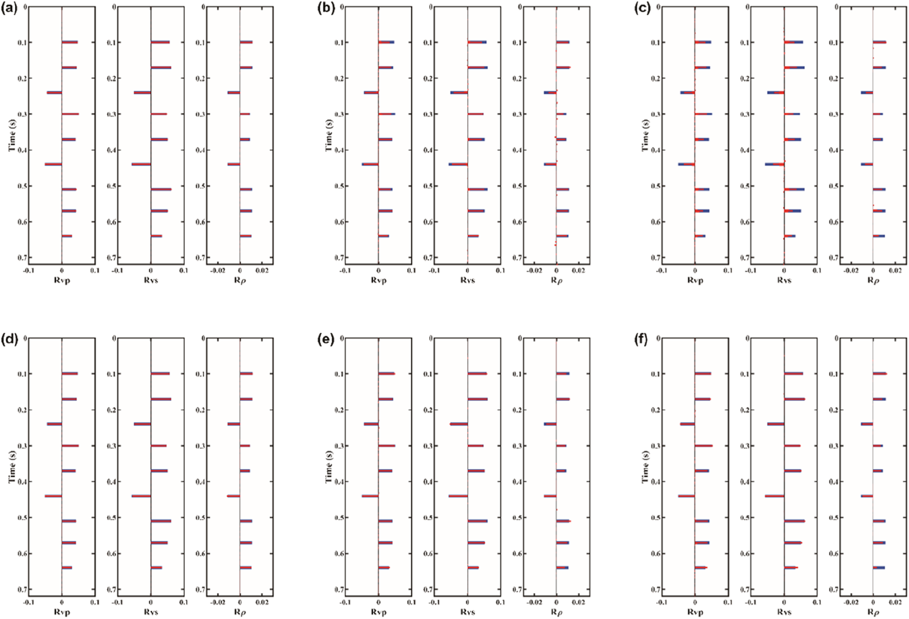
Figure 5. Comparison of three parameter reflection coefficient results for 1D multilayer model using different norm constraints: (a–c) results of noise-free, SNR = 10, and SNR = 5 with the L₁-norm constraint, respectively; (d–f) results of noise-free, SNR = 10, and SNR = 5 with the L_1-2 norm constraint, respectively. Each subfigure illustrates, from left to right, $v_{\mathrm{p}}$, $v_{\mathrm{s}}$, and $\rho$ reflection coefficients. The blue thick line and red thin line represent the true model reflection coefficients and the calculated reflection coefficients from the inversion results in Figure 3, respectively.

Well log data

In the well log model test, the model curves are shown in Figure 6a. The left panel shows the P-wave velocity, the middle panel shows the S-wave velocity, and the right panel shows the density, with a time of 600 ms and a time sampling interval of 2 ms. Using this model and applying approximate equations, reflection coefficients at different angles are calculated, with the maximum angle being 40°. These are then convolved with a Ricker wavelet of 40 Hz dominant frequency to generate the prestack angle gathers for both PP-wave and PS-wave data. Different levels of noise are added to the synthetic gathers, as shown in Figures 6b–d, representing noise-free, SNR = 10, and SNR = 5 conditions for the PP-wave and PS-wave prestack angle gathers, respectively.

Figure 6

Figure 6. 1D well log data and prestack synthetic angle gathers for PP- and PS-wave. (a) 1D well log data, (b) noise-free, (c) SNR = 10, (d) SNR = 5.

The synthetic angle gathers of PP- and PS-waves data from the well-log model are used directly for inversion tests. The results of only PP-wave inversion and PP-PS joint inversion are compared. Figure 7 shows the elastic parameter results under different signal-to-noise ratio, comparing the outcomes of only PP-wave inversion and PP-PS joint inversion. In the noise-free case, both only PP-wave and PP-PS joint inversion results match the true model. As the noise level increases, the inversion quality decreases, but the joint inversion consistently outperforms the only PP-wave inversion. Table 2 provides the correlation coefficients and normalized root mean square errors between the inversion results from Figure 7 and the true model. The table shows that the PP-PS joint inversion achieves higher correlation coefficients and lower root mean square errors, indicating that the accuracy of the PP-PS joint inversion is superior to that of the only PP-wave inversion.

Figure 7

Figure 7. Comparison of three parameter inversion results for the well log data: (a–c) results of noise-free, SNR = 10, and SNR = 5 with only PP-wave, respectively; (d–f) results of noise-free, SNR = 10, and SNR = 5 with joint PP- and PS-wave, respectively. Each subfigure illustrates, from left to right, the inversion results for $V_{\mathrm{P}}$, $V_{\mathrm{S}}$, and $\rho$. The black solid line, red solid line and blue dashed line represent the actual model, inversion result, and initial model, respectively.

Table 2

Table 2. Correlation coefficients and normalized root-mean-square errors between inversion results and the true model for the well log data.

Application to real field data

After testing with synthetic data, the proposed method is applied to real field seismic data, collected using Offshore Bottom Node (OBN) seismic acquisition. Compared to conventional towed-cable seismic acquisition, OBN places sensors on the seafloor, enabling effective collection of multi-component seismic data. These data have advantages such as broad bandwidth, high signal-to-noise ratio, and wide azimuth coverage, resulting in clearer imaging and greatly aiding offshore oil and gas exploration.

Before joint inversion, we conduct a feasibility analysis of joint inversion of seismic data through well-seismic calibration. Figures 8a,b show the PP-wave and PS-wave well-seismic calibration for a representative well in the actual study area. As shown in the figure, there is a good correspondence between PP wave, PS wave, and actual well log data. In the target gas reservoir interval, an amplitude anomaly, commonly referred to as a “bright spot,” is observed near the well on the PP-wave section, while such a feature is not visible on the PS-wave section. This difference between PP-wave and PS-wave responses provides useful information for reservoir identification. It is important to note that due to the different travel times of PP-wave and PS-wave, two separate time-depth relationships are used in the well-seismic calibration. Before conducting joint inversion, it is necessary to match PP wave and PS wave seismic data. Here, our matching process can be divided into two steps. The first step is time matching. Based on the P-wave and S-wave velocity models obtained during imaging, we calculate the velocity ratio and converted the PS-wave data from PS-time to PP-time. The second step is frequency matching. We adopt a Fourier scaling method, using the PP seismic wavelet as the reference wavelet, to correct the PS seismic wavelet frequency band to be consistent with the PP seismic wavelet. This not only improves the stability of the joint inversion, but also eliminates the wavelet distortion caused by the time domain conversion in the first step.

Figure 8

Figure 8. Well-seismic calibration for seismic data feasibility analysis of joint inversion. (a) PP-wave well-seismic calibration. (b) PS-wave well-seismic calibration.

Figures 9a–c show the partially stacked angle profiles of the matched PP-wave data at 12°, 25°, and 38° angles, respectively, while Figures 9d–f show the partially stacked angle profiles of the matched PS-wave data at the same angles. Comparing the matched results shows consistent timing between the PP-wave and PS-wave profiles. The seismic responses to the same geological structures also correspond well, indicating that the matched data meet the requirements for joint PP- and PS-waves inversion. It is notable that in the PP-wave profiles, bright spots and discontinuous horizons appear in the lower part due to the influence of gas reservoirs. In contrast, the PS-wave profiles, less affected by gas, exhibits more continuous layering. Therefore, jointing PP- and PS-waves data in inversion improves the accuracy of the results.

Figure 9

Figure 9. Partially stacked angle profiles of PP-wave data: (a) 12°, (b) 25°, (c) 38°. Partially stacked angle profiles of PS-wave data: (d) 12°, (e) 25°, (f) 38°.

The proposed method is applied to real field data for joint inversion of subsurface elastic parameters. For comparison, an only PP-waves inversion is also conducted. Figures 10a–c show the results of the only PP-wave inversion, which include P-wave velocity, S-wave velocity, and density. Figures 10d–f present the results of the joint inversion for the same parameters, with well log data incorporated. The $V_{\mathrm{P}}/V_{\mathrm{S}}$ velocity ratio, which is a key parameter for identifying favourable reservoirs, is calculated using the inverted P-wave and S-wave velocities, and the results of reservoir identification from the only PP-waves inversion are compared with those from the joint inversion.

Figure 10

Figure 10. Comparison of real field data inversion results: (a–c) results of $V_{\mathrm{P}}$, $V_{\mathrm{S}}$, and $\rho$ with only PP-wave, respectively; (d–f) results of $V_{\mathrm{P}}$, $V_{\mathrm{S}}$, and $\rho$ with joint PP- and PS-wave, respectively.

The comparison between the only PP-wave inversion and the PP-PS joint inversion shows that the trends in the P-wave velocity results are largely consistent, both aligning with the well log data. For S-wave velocity and density, the joint inversion incorporating PS-wave data offers greater lateral continuity in gas-bearing layers, better reflecting the characteristics of the rock skeleton and corresponding more closely to the well data. The velocity ratio profiles in Figure 11 highlight that the PP-PS joint inversion provides higher-resolution $V_{\mathrm{P}}/V_{\mathrm{S}}$ velocity ratios, which are more effective for distinguishing favourable reservoirs compared to the only PP-wave inversion.

Figure 11

Figure 11. Comparison of $V_{\mathrm{P}}/V_{\mathrm{S}}$ velocity ratio results: (a) only PP-wave inversion; (b) joint PP-, PS-wave inversion.

To further compare the effectiveness of only PP-wave inversion versus joint PP- and PS-wave inversion, this study conducts focused analyses on potential reservoirs. In the target study area, the reservoirs are predominantly gas-bearing formations where P-wave velocity exhibits rapid attenuation due to gas-saturated fluids, resulting in characteristic low $V_{\mathrm{P}}/V_{\mathrm{S}}$ value. $V_{\mathrm{P}}/V_{\mathrm{S}}$ profiles derived from inversion results are calculated and presented in Figure 12, with separate illustrations showing profiles obtained from only PP-wave inversion and joint PP- and PS-wave inversion approaches. This comparative visualization demonstrates the differential performance between the two inversion methodologies in capturing $V_{\mathrm{P}}/V_{\mathrm{S}}$ characteristics.

Figure 12

Figure 12. Comparison of $V_{\mathrm{P}}/V_{\mathrm{S}}$ velocity ratio results for the connected well survey line: (a) only PP-wave inversion; (b) joint PP-, PS-wave inversion.

To verify the reliability of the results, five well logs are incorporated into the figure. In the well log interpretation, distinct colors are employed to represent different reservoir interpretation outcomes, with gas-bearing reservoirs explicitly marked in red. A clear observation is that the $V_{\mathrm{P}}/V_{\mathrm{S}}$ derived from joint inversion demonstrates significantly higher spatial resolution compared to conventional only PP-wave inversion method. The low $V_{\mathrm{P}}/V_{\mathrm{S}}$ zones exhibit precise alignment with the gas-bearing reservoir intervals interpreted from the well logs, revealing strong spatial consistency. This high degree of correspondence validates the superior precision of the joint inversion approach.

This improvement primarily arises from the integration of PS-wave data in the joint inversion, which is inherently more sensitive to S-wave velocity variations. By incorporating PS-wave data, the joint inversion achieves enhanced precision in estimating S-wave velocities. Consequently, the velocity ratios calculated from the joint inversion results display higher fidelity, enabling more reliable reservoir characterization and fluid discrimination. Such advancements underscore the critical advantage of joint inversion in resolving complex subsurface features, particularly in gas-saturated environments where conventional only PP-wave inversion methods face limitations due to rapid velocity attenuation.

In Figure 13, the two purple-dashed horizons delineate two sets of potential sandstone reservoirs. $V_{\mathrm{P}}/V_{\mathrm{S}}$ slices extracted along these horizons are presented in Figures 14. Compared to $V_{\mathrm{P}}/V_{\mathrm{S}}$ slices derived from only PP-wave inversion, the slices obtained through joint inversion exhibit significantly enhanced clarity, demonstrating a superior ability to distinguish gas-bearing sandstone reservoirs. Beyond the drilling-validated locations, additional areas exhibit substantial potential for high-quality reservoirs, as highlighted by the joint inversion results. These findings provide critical insights for guiding future exploration and development activities.

Figure 13

Figure 13. Comparison of $V_{\mathrm{P}}/V_{\mathrm{S}}$ velocity ratio slice results for sand1 body: (a) only PP-wave inversion; (b) joint PP-, PS-wave inversion.

Figure 14

Figure 14. Comparison of $V_{\mathrm{P}}/V_{\mathrm{S}}$ velocity ratio results slice for sand2 body: (a) only PP-wave inversion; (b) joint PP-, PS-wave inversion.

Discussion and conclusion

We focused on the joint inversion of multi-wave seismic data. In the joint inversion of PP- and PS-wave information, a key point is how to properly combine the PP- and PS-wave reflection coefficients using an appropriate reflectivity equation. Moreover, how to ensure the stability and accuracy of the joint inversion is also an issue that requires thorough investigation and careful consideration. A joint inversion method for PP- and PS-waves prestack gathers is developed based on the Aki-Richards equations for PP-wave and PS-wave reflection coefficients. An L_1-2-norm constraint is introduced, and a detailed expression of the objective function is derived. The DCA + ADMM method is applied during the inversion process to solve the optimization problem for the joint inversion of PP- and PS-waves. In the synthetic data tests, the L_1-2-norm constraint is compared with conventional norm constraint method using a multilayer model. The results confirm that the L_1-2-norm provides stable and superior sparse constraint performance, making it more suitable for prestack seismic inversion. For joint inversion of PP- and PS-waves, this approach improves inversion accuracy. The method is applied to the actual well log data, comparing only PP-wave inversion with joint inversion. The results demonstrate that joint inversion offers higher accuracy and better noise resistance. In the application to real field data, a comparison is made between only PP-wave inversion and joint inversion with PP- and PS-waves. The results show that joint inversion outperforms only PP-wave inversion, providing better reservoir prediction and more accurate identification of favourable reservoirs. The proposed joint inversion method has achieved good results in reservoir characterization of offshore OBN seismic data. In addition to appropriate inversion methods, how to achieve high-precision matching between P- and S-wave data, and how to construct initial models are also issues that need to be noted in field practical data applications. Furthermore, multicomponent joint inversion directly in the depth domain is a key focus of future research.

Data availability statement

The data that support the findings of this study are available on request from the corresponding author (Y2hlbnNxQGN1cC5lZHUuY24=). The data are not publicly available due to their containing information that could compromise the privacy of research participants.

Author contributions

FL: Writing – review and editing. SL: Writing – review and editing. RW: Writing – original draft, Writing – review and editing. YT: Writing – original draft, Writing – review and editing. SC: Writing – original draft, Writing – review and editing.

Funding

The author(s) declare that financial support was received for the research and/or publication of this article. The research was supported by the National Natural Science Foundation of China (grant no. 42174130, 42474151).

Acknowledgments

We would like to thank the associate editor and two reviewers for their valuable comments.

Conflict of interest

Author FL, SL, RW, were employed by CNOOC (China) Limited Hainan Branch.

The remaining authors declare that the research was conducted in the absence of any commercial or financial relationships that could be construed as a potential conflict of interest.

Generative AI statement

The author(s) declare that no Generative AI was used in the creation of this manuscript.

Any alternative text (alt text) provided alongside figures in this article has been generated by Frontiers with the support of artificial intelligence and reasonable efforts have been made to ensure accuracy, including review by the authors wherever possible. If you identify any issues, please contact us.

Publisher’s note

All claims expressed in this article are solely those of the authors and do not necessarily represent those of their affiliated organizations, or those of the publisher, the editors and the reviewers. Any product that may be evaluated in this article, or claim that may be made by its manufacturer, is not guaranteed or endorsed by the publisher.

References

Aki, K., and Richards, P. G. (1980). Quantitative seismology: theory and methods. Freeman.

Google Scholar

Aster, R. C., Borchers, B., and Thurber, C. H. (2019). Parameter estimation and inverse problems. Elsevier. doi:10.1016/C2015-0-02458-3

CrossRef Full Text | Google Scholar

Avseth, P., and Lehocki, I. (2016). Combining burial history and rock-physics modeling to constrain AVO analysis during exploration. Lead. Edge 35 (6), 528–534. doi:10.1190/tle35060528.1

CrossRef Full Text | Google Scholar

Chai, X., Wang, S., Yuan, S., Zhao, J., Sun, L., and Wei, X. (2014). Sparse reflectivity inversion for nonstationary seismic data. Geophysics 79 (3), V93–V105. doi:10.1190/geo2013-0313.1

CrossRef Full Text | Google Scholar

Chen, H., Moradi, S., and Innanen, K. A. (2021). Joint inversion of frequency components of PP-and PSV-wave amplitudes for attenuation factors using second-order derivatives of anelastic impedance. Surv. Geophys. 42 (4), 961–987. doi:10.1007/s10712-021-09649-1

CrossRef Full Text | Google Scholar

Englehart, T., Randazzo, S., Bertagne, A., and Cafarelli, B. (2001). Interpretation of four-component seismic data in a gas cloud area of the central Gulf of Mexico. Lead. Edge 20 (4), 400–407. doi:10.1190/1.1438960

CrossRef Full Text | Google Scholar

Hu, G., Liu, Y., Wei, X., and Chen, T. (2011). Joint PP and PS AVO inversion based on bayes theorem. Appl. Geophys. 8 (4), 293–302. doi:10.1007/s11770-010-0306-0

CrossRef Full Text | Google Scholar

Huang, G., Chen, X., and Chen, Y. (2021). P-P and dynamic time warped P-SV wave AVA joint-inversion with ℓ1–2 regularization. IEEE Trans. Geoscience Remote Sens. 59 (7), 5535–5548. doi:10.1109/tgrs.2020.3022051

CrossRef Full Text | Google Scholar

Jin, S. (1999). Characterizing reservoir by using jointly P- and S-Wave AVO analyses. Houston, USA: SEG Technical Program Expanded Abstracts, Society of Exploration Geophysicists, 687–690. doi:10.1190/1.1821117

CrossRef Full Text | Google Scholar

Karimi, O., Omre, H., and Mohammadzadeh, M. (2010). Bayesian closed-skew Gaussian inversion of seismic AVO data for elastic material properties. Geophysics 75 (1), R1–R11. doi:10.1190/1.3299291

CrossRef Full Text | Google Scholar

Knapp, S., Payne, N., and Johns, T. (2001). Imaging through gas clouds: a case history from the gulf of Mexico: SEG technical program expanded abstracts. San Antonio, TX: Society of Exploration Geophysicists, 776–779. doi:10.1190/1.1816747

CrossRef Full Text | Google Scholar

Kurt, H. (2007). Joint inversion of AVA data for elastic parameters by bootstrapping. Comput. Geosci. 33 (3), 367–382. doi:10.1016/j.cageo.2006.08.012

CrossRef Full Text | Google Scholar

Larsen, J. A., Margrave, G. F., and Lu, H. (1999). AVO analysis by simultaneous P-P and P-S weighted stacking applied to 3C-3D seismic data. Houston, TX: SEG Technical Program Expanded Abstracts Society of Exploration Geophysicists, 721–724. doi:10.1190/1.1821127

CrossRef Full Text | Google Scholar

Li, Y., Alkhalifah, T., and Zhang, Z. (2021). Deep-learning assisted regularized elastic full waveform inversion using the velocity distribution information from wells. Geophys. J. Int. 226 (2), 1322–1335. doi:10.1093/gji/ggab162

CrossRef Full Text | Google Scholar

Lou, Y., Yin, P., He, Q., and Xin, J. (2015). Computing sparse representation in a highly coherent dictionary based on difference of L1 and L2. J. Sci. Comput. 64, 178–196. doi:10.1007/s10915-014-9930-1

Lu, J., Yang, Z., Wang, Y., and Shi, Y. (2015). Joint PP and PS AVA seismic inversion using exact Zoeppritz equations. Geophysics 80 (5), R239–R250. doi:10.1190/geo2014–0490.1

CrossRef Full Text | Google Scholar

Song, B., Zhi, L., Chen, S., Zeng, L., and Li, X. (2016). Nonlinear PP and PS joint inversion based on the Zoeppritz equations. Dallas, TX: SEG Technical Program Expanded Abstracts, Society of Exploration Geophysicists, 538–542. doi:10.1190/segam2016-13684445.1

CrossRef Full Text | Google Scholar

Stewart, R. R. (1990). Joint P and P-SV inversion: the CREWES Project research report, 2, 112–115.

Google Scholar

Stewart, R. R., Gaiser, J. E., Brown, R. J., and Lawton, D. C. (2002). Converted-wave seismic exploration: methods. Geophysics 67 (5), 1348–1363. doi:10.1190/1.1512781

CrossRef Full Text | Google Scholar

Tarantola, A. (2005). Inverse problem theory and methods for model parameter estimation. Philadelphia, PA: Society for Industrial and Applied Mathematics. doi:10.1137/1.9780898717921

CrossRef Full Text | Google Scholar

Taylor, H. L., Banks, S. C., and McCoy, J. F. (1979). Deconvolution with the ℓ1 norm. Geophys. 44 (1), 39–52. doi:10.1190/1.1440921

Veire, H. H., and Landrø, M. (2006). Simultaneous inversion of PP and PS seismic data. Geophysics 71 (3), R1–R10. doi:10.1190/1.2194533

CrossRef Full Text | Google Scholar

Wang, G., and Chen, S. (2022). Pre-stack seismic inversion with L_1-2-norm regularization via a proximal DC algorithm and adaptive strategy. Surv. Geophys. 43 (6), 1817–1843. doi:10.1007/s10712-022-09725-0

CrossRef Full Text | Google Scholar

Wang, Y., Ma, X., Zhou, H., and Chen, Y. (2018). L₁₋₂ minimization for exact and stable seismic attenuation compensation. Geophys. J. Int. 213 (3), 1629–1646. doi:10.1093/gji/ggy064

CrossRef Full Text | Google Scholar

Wang, L., Zhou, H., Wang, Y., Yu, B., Zhang, Y., Liu, W., et al. (2019). Three-parameter prestack seismic inversion based on L_1-2 minimization: geophysics, 84 5. R753–R766. doi:10.1190/geo2018-0730.1

CrossRef Full Text | Google Scholar

Wang, F., Huang, X., and Alkhalifah, T. (2023). A prior regularized full waveform inversion using generative diffusion models. IEEE Trans. geoscience remote Sens. 61, 1–11. doi:10.1109/TGRS.2023.3337014

CrossRef Full Text | Google Scholar

Xue, Y., Su, J., Geng, W., Chen, X., Feng, L., and Liang, Q. (2024). Entropy regularized nonlinear joint PP–PS AVO inversion using Zoeppritz equations. IEEE Trans. Geoscience Remote Sens. 62, 1–12. doi:10.1109/tgrs.2024.3388579

CrossRef Full Text | Google Scholar

Zhang, R., and Castagna, J. (2011). Seismic sparse-layer reflectivity inversion using basis pursuit decomposition. Geophysics 76 (6), R147–R158. doi:10.1190/geo2011-0103.1

CrossRef Full Text | Google Scholar

Zhi, L., Chen, S., Song, B., and Li, X. (2017). Nonlinear PP and PS joint inversion based on the exact Zoeppritz equations: a two-stage procedure. J. Geophys. Eng. 15 (2), 397–410. doi:10.1088/1742-2140/aa9a5c

CrossRef Full Text | Google Scholar