 Jianwei Liu1*
 Xiaoteng Pang1
 Haihua Jing1Mingwei Wang2Longhai Shen1
 Xiaohui Yan1Qin Zhang3
 Georgia Destouni4,5*
- 1School of Hydraulic Engineering, Dalian University of Technology, Dalian, China
- 2Liaoning Provincial Water Affairs Service Center, Liaoning Provincial Department of Water Resources, Shenyang, China
- 3Key Laboratory of Ecosystem Network Observation and Modeling, Institute of Geographic Sciences and Natural Resources Research, Chinese Academy of Sciences, Beijing, China
- 4Department of Physical Geography, Stockholm University, Stockholm, Sweden
- 5Department of Sustainable Development, Environmental Science and Engineering, KTH Royal Institute of Technology, Stockholm, Sweden
The climate change impacts on hydrological conditions may be strongly modulated by the spatial variability of the intensity of human activities within watersheds. Despite growing recognition of climate and anthropogenic influences on hydrological regimes, comprehensive and spatially explicit assessments remain limited, hindering the development of robust watershed management and climate adaptation strategies. In this study, we propose an integrated framework for such analysis and deciphering by combining principal component analysis, hydrological modeling, and a range of variability approach to diagnose and attribute hydrological regime changes. The framework is tested on the case of the Taoer River Basin as a representative watershed system with pronounced human-activity variation along the upstream to downstream direction. Our results show that human activities contribute only 18% to hydrological regime changes in the upstream regions, where anthropogenic influence is relatively low, compared to 49% in the downstream areas with substantially greater human interference. While the upstream areas exhibit more pronounced changes in daily maximum streamflow (78%–79%) and count of low pulses (79%), the downstream areas experience more substantial alterations in monthly average streamflow (84%–99%) and high pulse durations (85%). Overarching the human-activity variability, the climate change impacts increase the risk of flooding, while the human activities exert greater influence in amplifying drought risk. Simulations based on CMIP6 climate projections further indicate a significant increase in the likelihood of upstream flooding. Overall, our findings highlight the necessity of spatially differentiated management and adaptation strategies, tailored to steep human-activity gradients across watershed zones, to effectively address hydrological changes under climate stress.
1 Introduction
Hydrological regimes, as a key indicator of watershed ecological health, are highly sensitive to environmental changes (Ficklin et al., 2018). With the intensification of climate change and anthropogenic activities, these regimes may undergo significant alterations, affecting ecological, environmental, and socioeconomic services (Poff and Zimmerman, 2010; Sheikh et al., 2022). Such perturbations may manifest as increased risks of biodiversity loss (He et al., 2024), heightened water scarcity (Jenkins et al., 2021), and more frequent and severe flood and drought events (Wang H. et al., 2024). Therefore, understanding these changes at both regional and local scales is crucial for developing effective water resource management strategies (McMillan, 2021). Within a hydrological basin, upstream and downstream areas often differ markedly in terms of human activity intensity, ecological integrity, and hydrological response (Nkiaka and Okafor, 2024; Wang et al., 2023). Despite such spatial differences, many previous studies have analyzed watersheds as uniform entities, with limited attention to internal variability (Tian et al., 2019).
Effective watershed management requires comprehensive assessment of hydrological regimes in terms of alteration, drivers, and prediction. Previous research has explored these aspects, including selecting hydrological indicators for specific ecological targets and assessing historical changes (Fang et al., 2023); quantifying the contributions of various driving factors (Sheikh et al., 2022; McDowell et al., 2023); and utilizing hydrological models to predict future trends (Li J. et al., 2023). Previous studies have also shown that anthropogenic disturbances can cause spatially divergent hydrological responses within the same watershed (Levi et al., 2015). Nevertheless, few efforts have explicitly addressed the spatial variability of hydrological regime alterations, despite the fact that regime dynamics often exert greater ecological impact than absolute water availability (McDowell et al., 2023).
There are five key characteristics of hydrological regimes: magnitude, frequency, duration, timing, and rate of change (Rosenberg et al., 2000), with over 200 hydrological indicators developed for their quantification (Sheikh et al., 2022), including the well-known Indicators of Hydrologic Alteration (IHA) (Richter et al., 1996). However, many indicators exhibit autocorrelation and redundancy, which can introduce noise and compromise interpretability (Fang et al., 2023). Consequently, selecting an optimal subset of representative hydrologic indicators (RHIs) is a priority in hydrological assessments (Mims and Olden, 2013). Techniques such as principal component analysis (PCA) and autecology matrices have been employed to reduce redundancy among the 33 IHA indicators, helping to identify the most representative hydrological metrics (Suen et al., 2004).
Furthermore, understanding the spatial variability of hydrological regime and the drivers is crucial for identifying underlying mechanisms of hydrological evolution. Hydrological modeling is instrumental in capturing the spatial and temporal variability of hydrological regime (Eum et al., 2017; Mohammadi et al., 2024), by simulating diverse scenarios and representing different flow processes across various spatiotemporal scales and land areas (Horton et al., 2022), such as cold and tropical regions (Mohammadi et al., 2023; Msigwa et al., 2022), and upstream and downstream sections of a basin (Zang et al., 2012), over different temporal periods, including past, present, and future (Abbaszadeh et al., 2023; Stephens et al., 2019), and inter- or intra-annual scales (Mohammadi et al., 2022) and finer temporal resolutions (Azizi et al., 2021). The quantification separation methods for drivers include the Range of Variability Approach (RVA) (Richter et al., 1997), the Dundee Hydrologic Regime Alteration Method (DHRAM) (Black et al., 2005), Histogram Matching Approach (HMA) (Shiau and Wu, 2008), Histogram Comparison Approach (HCA) (Huang F. et al., 2017), etc. Among them, RVA derived from IHA, is widely used to quantify hydrological alterations (Berghuijs et al., 2017; Destouni et al., 2013; Guo et al., 2024). Studies have shown that hydrological changes can vary significantly across different areas within the same watershed, sometimes even exhibiting opposing trends (Li and Quiring, 2021). By integrating hydrological models with RVA, it is also possible to quantify the contribution of various drivers to hydrological regime changes across different spatial and temporal scales.
This study systematically investigate the spatial variability in hydrological regime evolution, underlying drivers, and projected future changes. To this end, the Taoer River Basin (TRB) (Figure 1) is used as a representative case study due to its pronounced distinct natural and human-induced disturbances in upstream and downstream regions. Our goal is to explore to what degree and how spatially variable human activities in watersheds drive distinct evolution and future trends of hydrological regimes. To achieve this, we integrate PCA, IHA, RVA, and hydrological modeling. First, PCA is applied to reduce redundancy in IHA indicators. Next, RVA and the Soil and Water Assessment Tool (SWAT) are combined to assess the spatiotemporal evolution of hydrological alterations and attribute changes to climate versus anthropogenic drivers Finally, SWAT and the Hydrologic Engineering Center’s Hydrologic Modeling System (HEC-HMS) are coupled with climate change projections of the Coupled Model Intercomparison Project Phase 6 (CMIP6) to explore future trends in both ordinary and extreme hydrological regimes under different Shared Socioeconomic Pathways (SSP) scenarios.
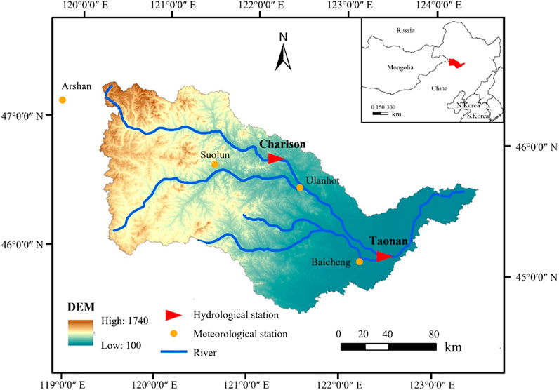
Figure 1. Geographic location and water system map of the Taoer River Basin (TRB).
2 Methods and materials
2.1 The research framework
The framework of the developed approach is shown in Figure 2. The framework integrates IHA, PCA, RVA, and hydrological modeling to arrive at the most important RHIs and the driving factors behind their changes, and to predict their future trends. Analysing the hydrological regimes in both upstream and downstream areas of the watershed, PCA is used to remove the redundancy in IHA, yielding the most important RHIs. Subsequently, using the SWAT model and referencing the RVA approach, the contribution of climate change and human activities to changes in hydrological regimes are quantitatively assessed separately for the upstream and downstream areas. Finally, based on CMIP6 outputs, the SWAT model and HEC-HMS are combined to project future trends in hydrological regimes under both general and extreme scenarios.
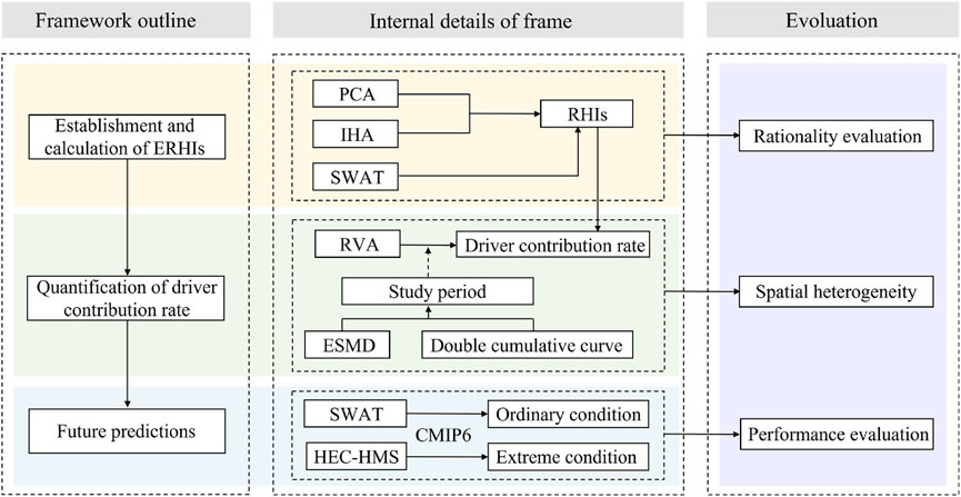
Figure 2. Framework for hydrological regime and predictions. RHIs, PCA, IHA, SWAT represent the most Representative Hydrologic Indicators, Principal Component Analysis, Indicators of Hydrologic Alteration, and Soil and Water Assessment Tool, respectively. RVA and ESMD represent Range of Variability Approach, and Extreme-point Symmetric Mode Decomposition method. CMIP6 and HEC-HMS represent Coupled Model Intercomparison Project Phase 6, and Hydrologic Engineering Center’s -Hydrologic Modeling System.
2.2 Hydrological models
This study applies SWAT and HEC-HMS to simulate hydrological regime. SWAT serves two functions to reflect the ordinary hydrological regime under long-term daily meteorological conditions in this study. First, it simulates the natural state of upstream and downstream areas from 1980 to 2014 to calculate values of RHIs. Second, it predicts the future ordinary conditions of the hydrological regime. HEC-HMS was further utilized to examine the extreme hydrological regime in the basin, i.e., flood processes at the hourly scale. The use of both SWAT and HEC-HMS stems from their differing strengths and applicable scenarios. Specifically, SWAT is widely used for watershed-scale modeling and long-term hydrological simulations but has limited capability in capturing short-term extremes (Ferreira et al., 2021; Geng et al., 2025). In contrast, HEC-HMS is better suited for fine temporal resolution and is more effective in simulating high-frequency extreme events such as floods (Kalakuntla and Umamahesh, 2025). Therefore, the combined use of both models allows for a complementary approach to better capture the full range of hydrological regime.
Operationally, the SWAT model for TRB was constructed using DEM, land use, soil, meteorological, and hydrological data. The upstream (Charlson) and downstream (Taonan) hydrological stations served as the outlets for the subbasins. The SUFI-2 algorithm was employed for model calibration and validation (Collins et al., 2022). The coefficient of determination (
There are four computational modules in HEC-HMS: Loss, Transform, Baseflow, and Rounting models (Chakraborty and Biswas, 2021). In this study, SCS Curve Number, SCS Unit Hydrograph, Recession, and Muskingum were selected for these four computational modules, respectively (Vafakhah et al., 2018). In addition, the simulation results were evaluated using four indexes: peak flow relative error (
2.3 Establishment and calculation of RHIs
For the 33 IHA indicators of the upstream and downstream areas of the TRB, PCA analysis was conducted. Indicators with eigenvalues greater than 1 and a cumulative contribution rate exceeding 80% were selected as principal components. The most frequently occurring indicators were then chosen to obtain the most important RHIs. The PCA method reduces dimensionality by transforming the original correlated variables to a smaller number of uncorrelated variables while retaining as much of the original data information as possible (Wang T. et al., 2024). Therefore, the principal components are these fewer comprehensive variables, which were selected as the RHIs to replace IHA in this study.
2.4 The change degree of RHIs
RVA was applied to the selected RHIs to calculate their change degree, including the degree of alteration for the
where
2.5 Quantification of driver contribution rate
Assuming that climate change and human activities are the two primary and independent drivers of runoff variation, and that their impacts on hydrological regimes are both linear and additive (Huang et al., 2024), the integrated change degree of RHIs for the observed runoff series was calculated using Equation 5:
where
The integrated change degrees due to climate change and human activities were calculated from Equations 6 and 7, respectively:
where
The contribution rates of climate change (
2.6 Future predictions
To inform adaptive water management and disaster mitigation under future climate change, this study further simulates hydrological regimes under both ordinary and extreme future scenarios. For ordinary hydrological regimes, the SWAT model was applied to characterized the conditions between the history period (1970–2014) and the future change period (2025–2060). To obtain temperature and precipitation conditions for future periods, we used output data from the TaiESM1 climate model under the SSP126, SSP245, and SSP585 scenarios. These data were further bias-corrected before used as input for the SWAT model, based on observed meteorological data for the reference period using the quantile mapping and the data assimilation method (Ngai et al., 2017; Reichle, 2008).
For extreme conditions, we used M3D precipitation data under the SSP245 scenario to analyze flood characteristics in the upstream areas of TRB for the future period 2025–2034. Historical floods in these upstream areas were primarily caused by prolonged precipitation events lasting around 72 h, so the duration of extreme precipitation was set at 3 days (Hiraga et al., 2025). To simulate flood processes under extreme precipitation, annual M3D precipitation was downscaled to hourly levels based on historical storm statistics (Trinh et al., 2022). The 1998 flood in the TRB, the most severe in the last 60 years, served as a reference for two future extreme precipitation scenarios:
Scenario A: Assuming that the temporal distribution of future M3D precipitation will follow a similar pattern to the storm events observed in the historical period, selected based on a matching criterion for similar total precipitation.
Scenario B: Assuming that the temporal distribution of future M3D precipitation is based on an unfavorable scenario, corresponding to the historical flood event on 9 July 1998.
3 Case study characteristics
3.1 Study area
The TRB (Figure 1) in northeastern China is the largest right-bank tributary of the Nenjiang River system, with a main stream length of approximately 563 km. The TRB is situated within a semiarid region, with temperate continental climate. Based on the records from 1958 to 2018, precipitation in TRB exhibits highly irregular spatiotemporal distribution patterns. The typical annual precipitation is currently 434 mm, with up to 83% of the total precipitation occurring between June and September. Geographically, downstream areas receive only 42.3% of the rainfall observed in upstream areas. In this study, the Charlson and Taonan hydrological stations were selected to represent the upstream and downstream extents of the study area, respectively. The TRB was chosen because of the significant spatial differences in land use and runoff processes in the basin (Liu et al., 2017).
3.2 Data
Runoff data for the TRB hydrological stations were sourced from the Hydrological Yearbook, comprising annual runoff data from 1958 to 2016 and daily runoff data from 1980 to 2014. Meteorological data for the Arxan, Suolun, Ulanhot, and Baicheng stations from 1970 to 2014 were obtained from the China Meteorological Data Service Center. Flood and corresponding storm data with a time step of 1 hour was obtained from the Songliao River Water Resources Commission of the Ministry of Water Resources.
Digital elevation models (DEM) with a spatial resolution of 30 × 30 m was downloaded from the Geospatial Data Cloud. Soil data with a spatial resolution of 1 × 1 km obtained from the Harmonized World Soil Database. Land use data from the Resource and Environment Sciences Data Platform. CMIP6 data with a spatial resolution of 288° × 192° was sourced from the Earth System Grid Federation.
4 Results
4.1 The selected RHIs
As illustrated in Figure 3, the eigenvalues of PC1∼PC8 at Charlson Station are greater than 1 and have a cumulative contribution rate of 92%. Similarly, the eigenvalues of PC1∼PC7 at Taonan Station are greater than 1 and have a cumulative contribution rate of 87%. The highest absolute loading values of IHA in the PCs for the Charlson and Taonan stations are taken as the main components of the upstream and downstream sections in the TRB, respectively. Consequently, the selected most important RHIs are the most frequent indicators for the two hydrological conditions. These are: mean value for January (MVJan), mean value for July (MVJul), maxima 3-day (M3D), julian date of 1 day maximum (JD1DM), low pulses count (LPC), high pulses duration (HPD), and fall rate (FR). Figure 4 shows that most of the correlation coefficients between these indicators are generally low, verifying the validity of the selected RHIs.
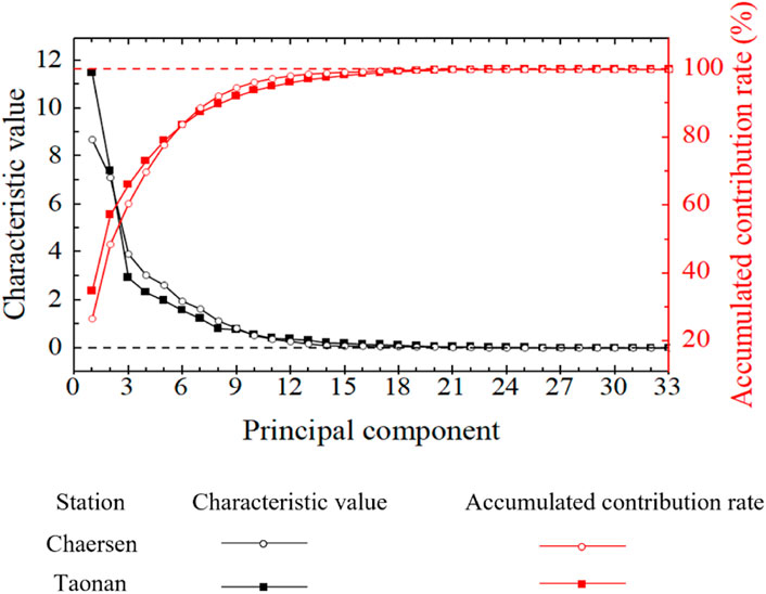
Figure 3. Principal component analysis (PCA) of indicators of hydrologic alteration (IHA).
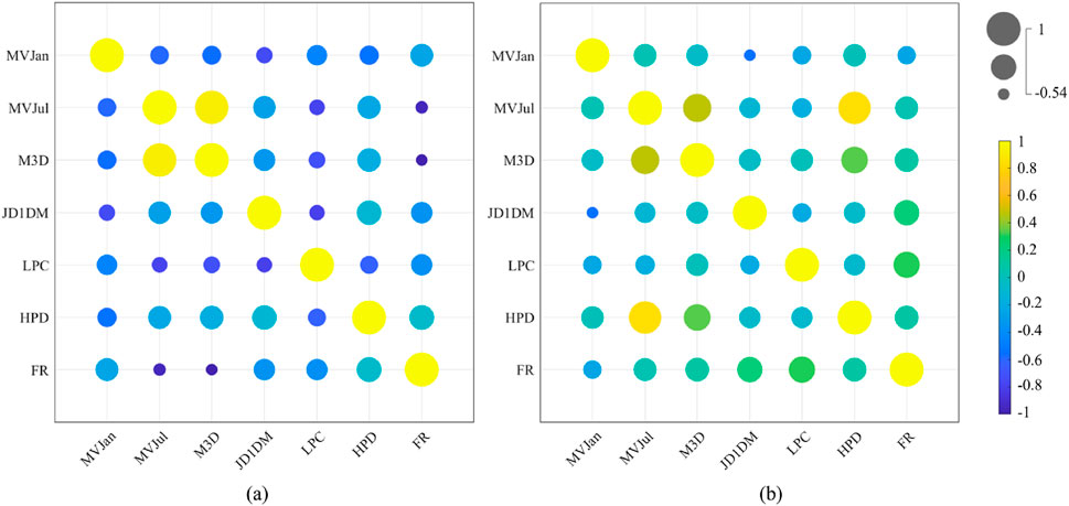
Figure 4. The correlation heatmap of the most representative hydrologic indicators (RHIs). (a) Charlson Station. (b) Taonan Station. MVJan, MVJul, M3D, JD1DM, HPD, LPC and FR represent the flow characteristics of mean value for January, mean value for July, maxima 3-day, julian date of 1-day maximum, high pulses duration, low pulses count and fall rate, respectively.
4.2 Spatially variable alterations and drivers of hydrological regime
Despite the decline trend and change point (in 1998) being identical for the upstream and the downstream runoff series, as determined by ESMD and double mass curve of rainfall-runoff (Figures 5–7), there are also important differences. The downstream section shows a significantly greater decline compared to the upstream section (Figure 5), and there were six change points (1963, 1967, 1973, 1979, 1983, and 1998) in the upstream annual runoff series while only four (1973, 1975, 1983, and 1998) in the downstream using ESMD (Figure 6). This suggests that the drivers may also differ. Based on these results, the study period is divided into the reference period relative to recent change (1980–1998) and the recent change period (1999–2014).
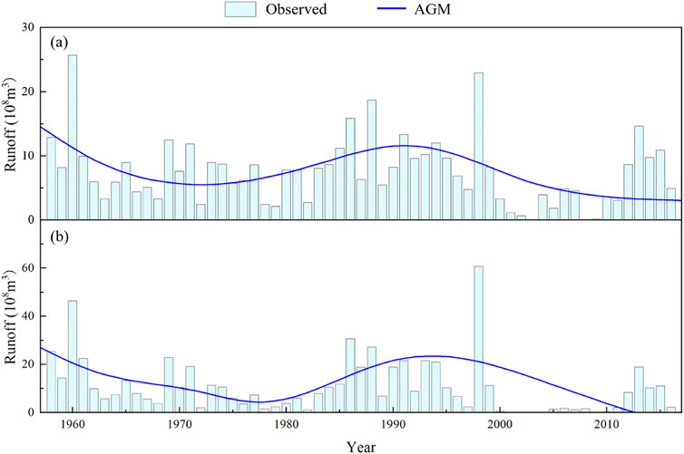
Figure 5. Observed annual runoff series and adaptive global mean (AGM) curve of the Taoer River Basin (TRB) from 1958 to 2016. (a) Charlson Station. (b) Taonan Station. AGM is the residual model obtained by Extreme-point Symmetric Mode Decomposition (ESMD) method to the observed annual runoff series.
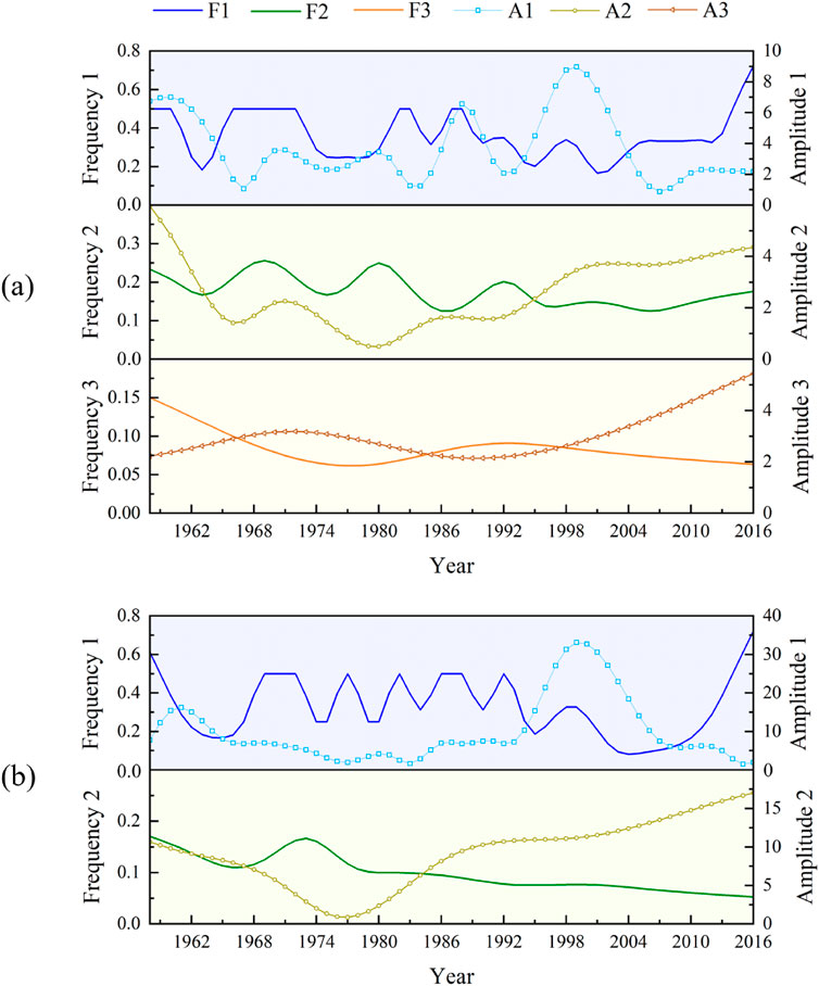
Figure 6. Time-varying amplitude-frequency of annual runoff series in the Taoer River Basin (TRB) from 1958 to 2016. (a) Charlson Station. (b) Taonan Station. The solid lines represent the frequency variations over time of each Intrinsic Mode Function (IMF) obtained through Extreme-point Symmetric Mode Decomposition (ESMD) method, while the symbol-lines represent the amplitude variations. The number of IMFs depends on the complexity of the extreme points, there were 36 and 32 extreme points in the upstream and downstream annual runoff series, respectively, with extreme point densities of 0.61 and 0.54. Thus, the number of IMFs for the annual runoff series at the upstream station is greater than that at the downstream station.
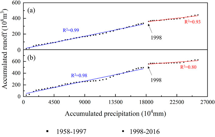
Figure 7. Rainfall-runoff double cumulative curve from 1958 to 2016. (a) Charlson Station. (b) Taonan Station.
The change degrees in flow characteristics from the reference period (1980–1998) to the change period (1999–2014) at Charlson and Taonan stations due to climate change alone (
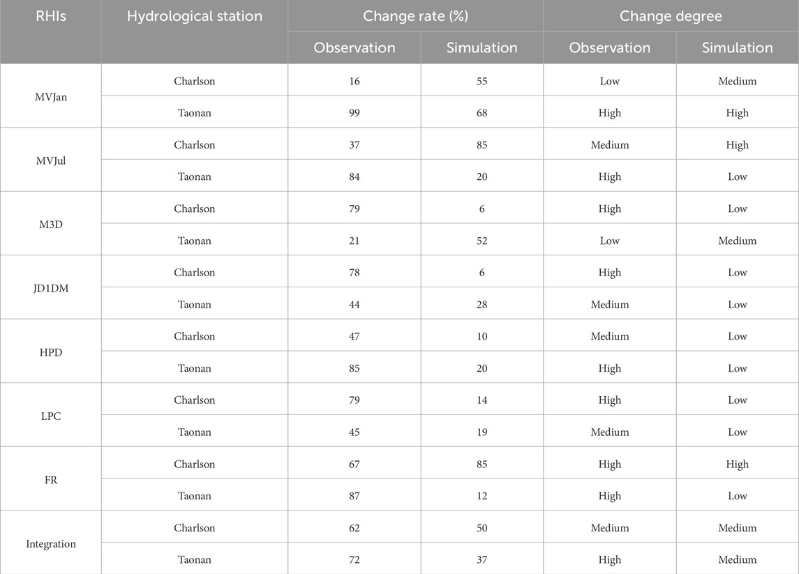
Table 1. Change degrees of RHIs at Charlson Station and Taonan Station in the TRB. MVJan, MVJul, M3D, JD1DM, HPD, LPC and FR represent the flow characteristics of mean value for January, mean value for July, maxima 3-day, julian date of 1-day maximum, high pulses duration, low pulses count and fall rate, respectively.
The resulting integrated change degrees of the RHIs for the observed and simulated series at Charlson Station are 62% and 50% (Table 1), respectively, with major changes emerging for daily maximum flow (79% M3D and 78% JD1DM) and LPC (79%). The contribution rates of climate change and human activities to the change at this station are 81% and 19%. Comparatively, Taonan Station exhibits dramatic decline in monthly mean flow (99% MVJan and 84% MV Jul) and HPD (85%). The integrated change degrees of the RHIs for the observed and simulated series at Taonan Station are 72% (high alteration) and 37% (moderate alteration), respectively. The contribution rates of climate change and human activities to the changes in the hydrological regime at this station are 51% and 49%, respectively.
4.3 Future ordinary and extreme hydrological regime
Figure 8 illustrates the resulting ordinary hydrological regime in the TRB under different future scenarios. These scenarios are obtained using the SWAT model, with climate data taken from the TaiESM1 climate model of CMIP6 and 2020 land use data as the underlying surface conditions. The results imply that the water volume during the flood season in both the upstream and the downstream areas of the TRB should be expected to decrease in the future. However, during the non-flood season, the upstream and downstream areas exhibit opposite trends. Compared to the baseline period (1980–2014), MVJan for the upstream areas is projected to decrease by 9%, 26%, and 52% under the SSP126, SSP245, and SSP585 scenarios, respectively. In contrast, the downstream MVJan is expected to increase by 231%, 169%, and 48% under the same scenarios.
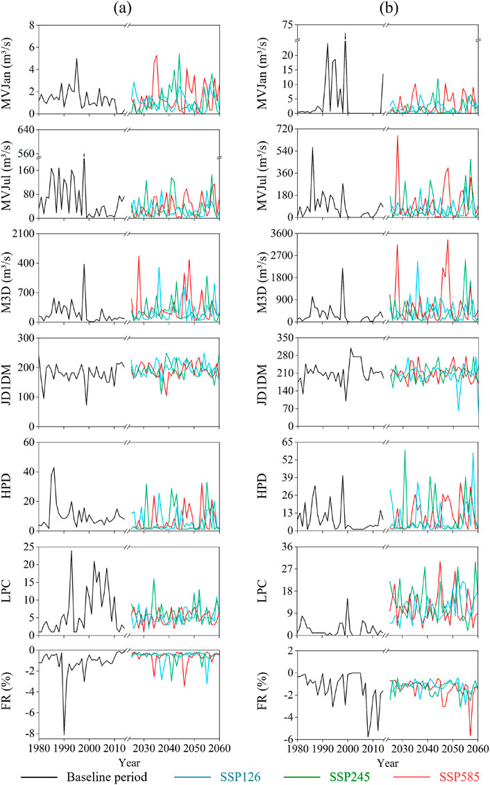
Figure 8. Characteristics of the most representative hydrologic indicators (RHIs) changes under different future scenarios of Taiwan Earth System Model (TaiESM1). (a) Charlson Station. (b)Taonan Station. MVJan, MVJul, M3D, JD1DM, HPD, LPC and FR represent the flow characteristics of mean value for January, mean value for July, maxima 3-day, julian date of 1-day maximum, high pulses duration, low pulses count and fall rate, respectively.
The change trends indicate possible reduction of future surface water availability in the basin. In contrast, the future M3D flows in both the upstream and downstream areas of the TRB are considerably higher than in the baseline period, with a notably increased frequency of high flows. It is this intensification of high flows that points to an increased future flood hazard in the future, particularly in the upstream areas.
Figure 9 and Table 2 show the resulting hydrological regime under the two future extreme precipitation scenarios. It can be observed that the total precipitation amounts vary across different years, leading to considerable differences in peak flows and flood volumes. This indicates that total precipitation amount is the dominant factor controlling flood response in the TRB. In contrast, the hydrographs for Scenario A and Scenario B are remarkably similar, suggesting that the flood response in the TRB is relatively insensitive to the temporal distribution of precipitation. Compared with the historical flood events, with an effective precipitation duration of approximately 3 days, the mean peak flows for the next 10 floods under Scenario A and B are expected to increase by 12.26% (43.0 m3/s) and 17.51% (61.4 m3/s), respectively, while the total mean flood volumes increase by 10.94% (17.3 million m3) and 11.06% (17.5 million m3), respectively.
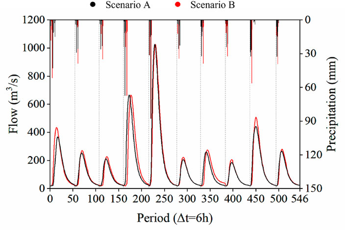
Figure 9. Future flood events under Scenario A and Scenario B. Scenario A distributes the design precipitation over time based on a historical storm event with a similar total rainfall amount. Scenario B distributes the design precipitation based on the most adverse conditions, using the historical storm event associated with the maximum flood. The vertical grey dashed lines in the figure demarcate flood events occurring in different future years.
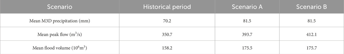
Table 2. Comparative analysis of flood features under different scenarios. M3D represent maxima 3-day.
5 Discussion
5.1 Contribution of the proposed framework
The initial advantage of this study is the simplification of IHA. The seven indicators included in the RHIs given by PCA are largely consistent with those selected in many previous studies (Gao et al., 2009). These indicators are considered to effectively capture key aspects of the hydrological regimes that impact ecosystems (Fang et al., 2023). The refined indicator system, after removing redundancies, is clearer and more efficient, facilitating the assessment of changes in hydrological regimes, their driving factors, and future trends within a watershed.
A second strength of this study lies in the complementary use of two hydrological models (SWAT and HEC-HMS) to analyze the spatial heterogeneity of hydrological regimes and their driving factors. Previous studies have also observed that the degrees of hydrological alteration vary, and in some cases even exhibit opposing trends, for different regions within the same watershed (Levi et al., 2015; Tian et al., 2019; Sarremejane et al., 2020; Li and Quiring, 2021). However, few studies have quantified the distinct driving factors or explored the underlying mechanisms behind the variations. Considering that ecological targets may also vary between upstream and downstream areas, calculating average drivers over an entire watershed may obscure several important spatial variations (Tian et al., 2019). These spatial nuances are essential for accurately capturing hydrological features and implementing effective water resource management strategies (Sarremejane et al., 2020). In comparison, separately calculating the drivers for upstream and downstream sections better elucidates important spatial heterogeneities within a watershed (Li and Quiring, 2021).
Few models can achieve satisfactory performance across multiple temporal scales (Huang S. et al., 2017). In this study, SWAT and HEC-HMS are employed in a complementary manner, each with distinct strengths: SWAT is well-suited for continuous watershed simulation with a strong emphasis on land use–hydrology interactions (Geng et al., 2025), whereas HEC-HMS is more appropriate for event-based modeling, focusing on rainfall–runoff transformation and flow routing (Kalakuntla and Umamahesh, 2025). Therefore, integrating models across multiple time scales and thoroughly assessing uncertainties are crucial steps for improving the accuracy of future hydrological forecasts. Daily-scale predictions of hydrological regime facilitate the study of long-term hydrological trends by reducing the influence of short-term extreme values (Brunner et al., 2020). However, masking of these short-term extremes may lead to neglect of crucial hydrological processes and events occurring at smaller time scales (McMillan, 2021), which could pose significant threats to life and property, such as floods (Rufat et al., 2015). Hourly-scale predictions can capture such sudden events and the hydrological impacts of extreme weather with short duration, in support of improved flood forecasting and decision-making (Dehghani et al., 2023).
Hydrological projections involve uncertainties from model structure (Herrera et al., 2022), parameterization (Hui et al., 2020), and climate model inputs (Chen et al., 2022). In terms of model structure, although some components rely on linear assumptions (Kollet et al., 2017), this study incorporates nonlinear modules such as the Green-Ampt infiltration method, the SCS Curve Number approach, and nonlinear reservoir routing. These selections, combined with event-specific parameterization and nonlinear variations in input data, help capture the complex feedback mechanisms of hydrological systems under both historical and future climate scenarios (Steinschneider et al., 2015). For parameter uncertainty, key sensitive parameters were selected based on previous studies, including CN, ESCO, and CH_K in SWAT (Liu et al., 2024), and initial abstraction and impervious in HEC-HMS (Acuña-Alonso et al., 2024). Calibration using multi-site observations and historical extreme events helped reduce uncertainty in parameter identification and estimation. To reduce uncertainty from climate model inputs (Zhang et al., 2025), this study applied various methods including quantile mapping to correct biases in precipitation and temperature simulations (Supplementary Methods S3). Climate models were selected based on their historical performance to minimize systematic errors and improve the reliability of future hydrological projections (Ahmed et al., 2019; Yang et al., 2021).
5.2 Spatial heterogeneity and management implications
In this study, spatial heterogeneity is primarily reflected in two aspects. First, the dominant drivers of hydrological regime change differ between the upstream and downstream sections of the TRB. In the upstream section, the hydrological regime in the is predominantly influenced by climate change, while the downstream section is affected by the combined impacts of climate change and human activities. The differing contributions can be attributed to several reasons: 1) human activities are less prevalent in upstream areas (Liang et al., 2010); 2) downstream areas have lower flow velocities, which may make them more susceptible to human impacts (Zhang et al., 2017); and 3) downstream ecosystems have lower stability due to additional change factors, such as land use changes (Li M. et al., 2023). For example, the downstream area includes extensive agricultural land and urban settlements, with substantial industrial and domestic water use. Second, the hydrological responses themselves show contrasting patterns upstream, the maximum daily flow increases due to climate change while downstream, the average monthly flow decreases due to human activities. This reflects two distinct directions in which climate change and human activities may increase extreme events.
Our projections for the TRB indicate that peak flood flows increase with precipitation concentration and intensity, which may be due to decreased soil infiltration and associated increased runoff intensity. Peak flows and total flood volumes may thus be expected increase, while the majority of flood events in the upstream areas of the TRB case study are projected to be small and medium scale over the next decade under the M3D precipitation scenario. Consequently, given the safety utilization of floodwater resources, it may be possible to alleviate the water supply-demand imbalance within the basin (Binns, 2022). Notably, the trends in hydrological indices between the upstream and downstream sections of the TRB are not entirely consistent and, in some cases, even opposite (Figure 8). This highlights the importance of adopting a region-specific approach to managing water resources (Huang and Swain, 2022).
This finding has important implications for watershed management. Given the marked differences in hydrological response mechanisms between upstream and downstream regions, uniform water resource policies may fail to address localized needs and could even lead to unintended consequences downstream (Zhao et al., 2023). It is therefore essential to promote region-specific management strategies: upstream areas should prioritize enhancing natural water retention and ecosystem conservation, while downstream regions require improvements in water-use efficiency and risk mitigation capacity. In addition, local stakeholders should be actively involved in climate-adaptive water management, enabling the integration of monitoring data and scenario-based forecasts to support dynamic, resilient, and coordinated basin governance.
5.3 Limitations and prospects
Despite the significant progress made in identifying the drivers of hydrological change and projecting future scenarios, several limitations remain. First, the attribution analysis assumes that climate change and human activities are the two primary and independent drivers of runoff variation, with linear and additive effects (Huang et al., 2024). However, interactions between climate and human influences in real-world hydrological processes are likely more complex, potentially involving nonlinear and synergistic effects (Yuan et al., 2017). Second, the SWAT and HEC-HMS models applied in this study rely in part on linear assumptions to simulate hydrological processes (Kollet et al., 2017). Under changing environmental conditions, key processes such as infiltration, runoff generation, and flow routing may exhibit pronounced nonlinear behaviors, which could compromise simulation accuracy. Third, the future hydrological scenarios were based primarily on optimal climate models under different SSPs, without a systematic assessment of the uncertainties arising from inter-model variability. Future research should incorporate more sophisticated models that capture climate–human interactions, explore the role of nonlinear processes in shaping hydrological responses, and, when selecting specific RHIs for ecological targets, such as fish diversity and abundance, it is essential to consider hydrological-ecological response relationships and underlying mechanisms in addition to the results from PCA (Mims and Olden, 2013; Yang et al., 2008).
6 Conclusion
In this study, we have developed and applied a general modeling framework to assess hydrological regime response and quantify spatiotemporal variability in past-to-future environments and the associated main change drivers. The proposed framework, which integrates PCA, IHA, RVA, SWAT and HEC-HMS, has identified major differences in the degrees of hydrological regime changes, and their driving factors, and future trends between the upstream and downstream regions of the test case study of TRB. Failure to consider the spatial variability of hydrological regimes within a watershed can lead to inefficient water management strategies.
This study has employed the SWAT and HEC-HMS hydrological models to project both ordinary and extreme future hydrological regimes, addressing the limitations of traditional daily-scale predictions using only SWAT. Overcoming these limitations may be vital for water resource planning and real-time management, particularly in basins with recurrent seasonal flooding. Additionally, the uncertainties in future climate scenarios and underlying models and assumptions, along with other important change trends, e.g., in land use, will also influence the relevance, accuracy, and uncertainties of future hydrological projections. Even with such uncertainties, however, this study has shown that accounting for the spatial variability of human activities within watersheds can give valuable insights and considerably improve the relevance and accuracy of hydrological change estimation, projection, and adaptation.
Data availability statement
The datasets presented in this study can be found in online repositories. The names of the repository/repositories and accession number(s) can be found below: https://github.com/Tunstall7/data.
Author contributions
JL: Conceptualization, Validation, Writing – review and editing, Methodology, Resources. XP: Formal Analysis, Writing – review and editing, Writing – original draft. HJ: Visualization, Formal Analysis, Supervision, Writing – review and editing. MW: Visualization, Software, Data curation, Writing – review and editing. LS: Writing – review and editing, Investigation. XY: Writing – review and editing. QZ: Writing – review and editing, Formal Analysis. GD: Funding acquisition, Writing – review and editing.
Funding
The author(s) declare that financial support was received for the research and/or publication of this article. JL was supported by the National Nature Science Foundation of China (Grant No. 52309079).
Conflict of interest
The authors declare that the research was conducted in the absence of any commercial or financial relationships that could be construed as a potential conflict of interest.
Generative AI statement
The author(s) declare that no Generative AI was used in the creation of this manuscript.
Any alternative text (alt text) provided alongside figures in this article has been generated by Frontiers with the support of artificial intelligence and reasonable efforts have been made to ensure accuracy, including review by the authors wherever possible. If you identify any issues, please contact us.
Publisher’s note
All claims expressed in this article are solely those of the authors and do not necessarily represent those of their affiliated organizations, or those of the publisher, the editors and the reviewers. Any product that may be evaluated in this article, or claim that may be made by its manufacturer, is not guaranteed or endorsed by the publisher.
Supplementary material
The Supplementary Material for this article can be found online at: https://www.frontiersin.org/articles/10.3389/feart.2025.1656661/full#supplementary-material
References
Abbaszadeh, M., Bazrafshan, O., Mahdavi, R., Sardooi, E. R., and Jamshidi, S. (2023). Modeling future hydrological characteristics based on land use/land cover and climate changes using the SWAT model. Water Resour. Manag. 37, 4177–4194. doi:10.1007/s11269-023-03545-6
Acuña-Alonso, C., Álvarez, X., Bezak, N., and Zupanc, V. (2024). Modelling the impact land use change on flood risk: Umia (Spain) and Voglajna (Slovenia) case studies. Ecol. Eng. 200, 107185. doi:10.1016/j.ecoleng.2024.107185
Ahmed, K., Sachindra, D. A., Shahid, S., Demirel, M. C., and Chung, E.-S. (2019). Selection of multi-model ensemble of general circulation models for the simulation of precipitation and maximum and minimum temperature based on spatial assessment metrics. Hydrol. Earth Syst. Sci. 23, 4803–4824. doi:10.5194/hess-23-4803-2019
Azizi, S., Ilderomi, A. R., and Noori, H. (2021). Investigating the effects of land use change on flood hydrograph using HEC-HMS hydrologic model (case study: Ekbatan Dam). Nat. Hazards 109, 145–160. doi:10.1007/s11069-021-04830-6
Berghuijs, W. R., Larsen, J. R., van Emmerik, T. H. M., and Woods, R. A. (2017). A global assessment of runoff sensitivity to changes in precipitation, potential evaporation, and other factors. Water Resour. Res. 53, 8475–8486. doi:10.1002/2017WR021593
Binns, A. D. (2022). Sustainable development and flood risk management. J. Flood Risk Manag. 15, e12807. doi:10.1111/jfr3.12807
Black, A. R., Rowan, J. S., Duck, R. W., Bragg, O. M., and Clelland, B. E. (2005). DHRAM: a method for classifying river flow regime alterations for the EC water framework directive. Aquat. Conserv. 15, 427–446. doi:10.1002/aqc.707
Brunner, M. I., Melsen, L. A., Newman, A. J., Wood, A. W., and Clark, M. P. (2020). Future streamflow regime changes in the United States: assessment using functional classification. Hydrol. Earth Syst. Sci. 24, 3951–3966. doi:10.5194/hess-24-3951-2020
Chakraborty, S., and Biswas, S. (2021). Simulation of flow at an ungauged river site based on HEC-HMS model for a Mountainous River Basin. Arab. J. Geosci. 14, 2080. doi:10.1007/s12517-021-08385-5
Chen, C., Gan, R., Feng, D., Yang, F., and Zuo, Q. (2022). Quantifying the contribution of SWAT modeling and CMIP6 inputting to streamflow prediction uncertainty under climate change. J. Clean. Prod. 364, 132675. doi:10.1016/j.jclepro.2022.132675
Collins, B., Najeeb, U., Luo, Q., and Tan, D. K. Y. (2022). Contribution of climate models and APSIM phenological parameters to uncertainties in spring wheat simulations: application of SUFI-2 algorithm in Northeast Australia. J. Agron. Crop Sci. 208, 225–242. doi:10.1111/jac.12575
Dehghani, A., Moazam, H. M. Z. H., Mortazavizadeh, F., Ranjbar, V., Mirzaei, M., Mortezavi, S., et al. (2023). Comparative evaluation of LSTM, CNN, and ConvLSTM for hourly short-term streamflow forecasting using deep learning approaches. Ecol. Inf. 75, 102119. doi:10.1016/j.ecoinf.2023.102119
Destouni, G., Jaramillo, F., and Prieto, C. (2013). Hydroclimatic shifts driven by human water use for food and energy production. Nat. Clim. Chang. 3, 213–217. doi:10.1038/nclimate1719
Eum, H.-I., Dibike, Y., and Prowse, T. (2017). Climate-induced alteration of hydrologic indicators in the Athabasca River basin, Alberta, Canada. J. Hydrol. 544, 327–342. doi:10.1016/j.jhydrol.2016.11.034
Fang, G., Yan, M., Dai, L., Huang, X., Zhang, X., and Lu, Y. (2023). Improved indicators of hydrological alteration for quantifying the dam-induced impacts on flow regimes in small and medium-sized rivers. Sci. Total Environ. 867, 161499. doi:10.1016/j.scitotenv.2023.161499
Ferreira, R. G., Dias, R. L. S., de Siqueira Castro, J., dos Santos, V. J., Calijuri, M. L., and da Silva, D. D. (2021). Performance of hydrological models in fluvial flow simulation. Ecol. Inf. 66, 101453. doi:10.1016/j.ecoinf.2021.101453
Ficklin, D. L., Abatzoglou, J. T., Robeson, S. M., Null, S. E., and Knouft, J. H. (2018). Natural and managed watersheds show similar responses to recent climate change. Proc Natl Acad Sci U. S. A. 115, 8553–8557. doi:10.1073/pnas.1801026115
Gao, Y., Vogel, R. M., Kroll, C. N., Poff, N. L., and Olden, J. D. (2009). Development of representative indicators of hydrologic alteration. J. Hydrol. 374, 136–147. doi:10.1016/j.jhydrol.2009.06.009
Geng, X., Lei, X., Song, X., Zhang, J., and Liu, W. (2025). Impact of human activities on the propagation dynamics from meteorological to hydrological drought in the Nenjiang River Basin, Northeast China. J. Hydrol. Reg. Stud. 58, 102214. doi:10.1016/j.ejrh.2025.102214
Guo, W., Wang, G., Ma, Y., Hong, F., Huang, L., Yang, H., et al. (2024). Evaluation of hydrological regime alteration and ecological flow processes in the changing environment of the Jialing River, China. J. Water Clim. Chang. 15, 978–997. doi:10.2166/wcc.2024.402
He, N., Guo, W., Lan, J., Yu, Z., and Wang, H. (2024). The impact of human activities and climate change on the eco-hydrological processes in the Yangtze River basin. J. Hydrol. Reg. Stud. 53, 101753. doi:10.1016/j.ejrh.2024.101753
Herrera, P. A., Marazuela, M. A., and Hofmann, T. (2022). Parameter estimation and uncertainty analysis in hydrological modeling. Wires. Water 9, e1569. doi:10.1002/wat2.1569
Hiraga, Y., Tahara, R., and Meza, J. (2025). A methodology to estimate probable maximum precipitation (PMP) under climate change using a numerical weather model. J. Hydrol. 652, 132659. doi:10.1016/j.jhydrol.2024.132659
Horton, P., Schaefli, B., and Kauzlaric, M. (2022). Why do we have so many different hydrological models? A review based on the case of Switzerland. Wiley Interdiscip. Rev.-Water 9 (9), e1574. doi:10.1002/wat2.1574
Huang, X., and Swain, D. L. (2022). Climate change is increasing the risk of a California megaflood. Sci. Adv. 8, eabq0995. doi:10.1126/sciadv.abq0995
Huang, Y., Zhang, K., Chao, L., Shi, W., and Huang, B. (2024). Development of a comprehensive framework for quantifying the collective and individual influence of climate change and human activities on hydrological regimes. Ecol. Indic. 166, 112487. doi:10.1016/j.ecolind.2024.112487
Huang, F., Li, F., Zhang, N., Chen, Q., Qian, B., Guo, L., et al. (2017). A histogram comparison approach for assessing hydrologic regime alteration. River Res. Appl. 33, 809–822. doi:10.1002/rra.3130
Huang, S., Kumar, R., Flörke, M., Yang, T., Hundecha, Y., Kraft, P., et al. (2017). Evaluation of an ensemble of regional hydrological models in 12 large-scale river basins worldwide. Clim. Change. 141, 381–397. doi:10.1007/s10584-016-1841-8
Hui, J., Wu, Y., Zhao, F., Lei, X., Sun, P., Singh, S. K., et al. (2020). Parameter optimization for uncertainty reduction and simulation improvement of hydrological modeling. Remote Sens-Basel 12, 4069. doi:10.3390/rs12244069
Jenkins, K., Dobson, B., Decker, C., and Hall, J. W. (2021). An integrated framework for risk-based analysis of economic impacts of drought and water scarcity in England and Wales. Water Resour. Res. 57, e2020WR027715. doi:10.1029/2020WR027715
Kalakuntla, N. T., and Umamahesh, N. V. (2025). A comprehensive evaluation of calibration strategies for flood prediction in a large catchment using HEC-HMS. Model Earth Syst. Environ. 11, 32. doi:10.1007/s40808-024-02276-w
Kollet, S., Sulis, M., Maxwell, R. M., Paniconi, C., Putti, M., Bertoldi, G., et al. (2017). The integrated hydrologic model intercomparison project, IH-MIP2: a second set of benchmark results to diagnose integrated hydrology and feedbacks. Water Resour. Res. 53, 867–890. doi:10.1002/2016WR019191
Levi, L., Jaramillo, F., Andričević, R., and Destouni, G. (2015). Hydroclimatic changes and drivers in the Sava River catchment and comparison with Swedish catchments. Ambio 44, 624–634. doi:10.1007/s13280-015-0641-0
Li, Z., and Quiring, S. M. (2021). Identifying the dominant drivers of hydrological change in the contiguous United States. Water Resour. Res. 57, e2021WR029738. doi:10.1029/2021WR029738
Li, Z., and Zhang, X. (2024). A novel coupled model for monthly rainfall prediction based on ESMD-EWT-SVD-LSTM. Manag 38, 3297–3312. doi:10.1007/s11269-024-03815-x
Li, J., Li, Y., Zhang, T., and Feng, P. (2023). Research on the future climate change and runoff response in the mountainous area of Yongding watershed. J. Hydrol. 625, 130108. doi:10.1016/j.jhydrol.2023.130108
Li, M., Gu, H., Wang, H., Wang, Y., and Chi, B. (2023). Quantifying the impact of climate variability and human activities on streamflow variation in Taoer River Basin, China. Environ. Sci. Pollut. Res. 30, 56425–56439. doi:10.1007/s11356-023-26271-3
Liang, L., Li, L., and Liu, Q. (2010). Temporal variation of reference evapotranspiration during 1961–2005 in the Taoer River basin of Northeast China. Agric. For. Meteorol. 150, 298–306. doi:10.1016/j.agrformet.2009.11.014
Liu, C., Sui, J., He, Y., and Hirshfield, F. (2013). Changes in runoff and sediment load from major Chinese rivers to the Pacific Ocean over the period 1955–2010. Int. J. Sediment. Res. 28, 486–495. doi:10.1016/S1001-6279(14)60007-X
Liu, J., Zhang, C., Kou, L., and Zhou, Q. (2017). Effects of climate and land use changes on water resources in the Taoer River. Adv. Meteorol. 2017, 1–13. doi:10.1155/2017/1031854
Liu, J., Pang, X., Yan, X., Chen, X., Wang, M., Ma, R., et al. (2024). A synergistic framework for dynamic water scarcity assessment: integrated blue and green water. J. Water Clim. Change. 15, 2379–2401. doi:10.2166/wcc.2024.728
McDowell, N. G., Anderson-Teixeira, K., Biederman, J. A., Breshears, D. D., Fang, Y., Fernández-de-Uña, L., et al. (2023). Ecohydrological decoupling under changing disturbances and climate. One Earth 6, 251–266. doi:10.1016/j.oneear.2023.02.007
McMillan, H. K. (2021). A review of hydrologic signatures and their applications. Wiley Interdiscip. Rev.-Water. 8, e1499. doi:10.1002/wat2.1499
Mims, M. C., and Olden, J. D. (2013). Fish assemblages respond to altered flow regimes via ecological filtering of life history strategies. Freshw. Biol. 58, 50–62. doi:10.1111/fwb.12037
Mohammadi, B., Safari, M. J. S., and Vazifehkhah, S. (2022). IHACRES, GR4J and MISD-based multi conceptual-machine learning approach for rainfall-runoff modeling. Sci. Rep. 12, 12096. doi:10.1038/s41598-022-16215-1
Mohammadi, B., Gao, H., Feng, Z., Pilesjö, P., Cheraghalizadeh, M., and Duan, Z. (2023). Simulating glacier mass balance and its contribution to runoff in Northern Sweden. J. Hydrol. 620, 129404. doi:10.1016/j.jhydrol.2023.129404
Mohammadi, B., Vazifehkhah, S., and Duan, Z. (2024). A conceptual metaheuristic-based framework for improving runoff time series simulation in glacierized catchments. Eng. Appl. Artif. Intell. 127, 107302. doi:10.1016/j.engappai.2023.107302
Molina-Navarro, E., Andersen, H. E., Nielsen, A., Thodsen, H., and Trolle, D. (2017). The impact of the objective function in multi-site and multi-variable calibration of the SWAT model. Environ. Modell. Softw. 93, 255–267. doi:10.1016/j.envsoft.2017.03.018
Msigwa, A., Chawanda, C. J., Komakech, H. C., Nkwasa, A., and van Griensven, A. (2022). Representation of seasonal land use dynamics in SWAT+ for improved assessment of blue and green water consumption. Hydrol. Earth Syst. Sci. 26, 4447–4468. doi:10.5194/hess-26-4447-2022
Ngai, S. T., Tangang, F., and Juneng, L. (2017). Bias correction of global and regional simulated daily precipitation and surface mean temperature over Southeast Asia using quantile mapping method. Glob. Planet. Change 149, 79–90. doi:10.1016/j.gloplacha.2016.12.009
Nkiaka, E., and Okafor, G. C. (2024). Changes in climate, vegetation cover and vegetation composition affect runoff generation in the Gulf of Guinea Basin. Hydrol. Process. 38, e15124. doi:10.1002/hyp.15124
Poff, N. L., and Zimmerman, J. K. H. (2010). Ecological responses to altered flow regimes: a literature review to inform the science and management of environmental flows. Freshw. Biol. 55, 194–205. doi:10.1111/j.1365-2427.2009.02272.x
Reichle, R. H. (2008). Data assimilation methods in the Earth sciences. Adv. Water Resour. 31, 1411–1418. doi:10.1016/j.advwatres.2008.01.001
Richter, B. D., Baumgartner, J. V., Powell, J., and Braun, D. P. (1996). A method for assessing hydrologic alteration within ecosystems. Conserv. Biol. 10, 1163–1174. doi:10.1046/j.1523-1739.1996.10041163.x
Richter, B., Baumgartner, J., Wigington, R., and Braun, D. (1997). How much water does a river need? Freshw. Biol. 37, 231–249. doi:10.1046/j.1365-2427.1997.00153.x
Rosenberg, D., McCully, P., and Pringle, C. (2000). Global-Scale environmental effects of hydrological alterations: introduction. Bioscience 50, 746–751. doi:10.1641/0006-3568(2000)050[0746:GSEEOH]2.0.CO;2
Rufat, S., Tate, E., Burton, C. G., and Maroof, A. S. (2015). Social vulnerability to floods: review of case studies and implications for measurement. Int. J. Disaster Risk Reduct. 14, 470–486. doi:10.1016/j.ijdrr.2015.09.013
Sarremejane, R., England, J., Sefton, C. E. M., Parry, S., Eastman, M., and Stubbington, R. (2020). Local and regional drivers influence how aquatic community diversity, resistance and resilience vary in response to drying. Oikos 129, 1877–1890. doi:10.1111/oik.07645
Sheikh, V., Sadoddin, A., Najafinejad, A., Zare, A., Hollisaz, A., Siroosi, H., et al. (2022). The density difference and weighted RVA approaches for assessing hydrologic regime alteration. J. Hydrol. 613, 128450. doi:10.1016/j.jhydrol.2022.128450
Shiau, J., and Wu, F. (2008). A Histogram matching approach for assessment of flow regime alteration: application to environmental flow optimization. River Res. Appl. 24, 914–928. doi:10.1002/rra.1102
Steinschneider, S., Wi, S., and Brown, C. (2015). The integrated effects of climate and hydrologic uncertainty on future flood risk assessments. Hydrol. Process. 29, 2823–2839. doi:10.1002/hyp.10409
Stephens, C. M., Marshall, L. A., and Johnson, F. M. (2019). Investigating strategies to improve hydrologic model performance in a changing climate. J. Hydrol. 579, 124219. doi:10.1016/j.jhydrol.2019.124219
Suen, J.-P., Herricks, E. E., and Eheart, J. W. (2004). “Ecohydrologic indicators for Rivers of Northern Taiwan,” in Paper presented at ASCE/EWRI world water and environmental resources Congress 2004. Salt Lake City, Utah: American Society of Civil Engineers. doi:10.1061/40737(2004)143
Tian, X., Zhao, G., Mu, X., Zhang, P., Tian, P., Gao, P., et al. (2019). Hydrologic alteration and possible underlying causes in the Wuding River, China. Sci. Total Environ. 693, 133556. doi:10.1016/j.scitotenv.2019.07.362
Trinh, T., Iseri, Y., Diaz, A. J., Snider, E. D., Anderson, M. L., and Levent Kavvas, M. (2022). Maximization of historical storm events over seven watersheds in Central/Southern Sierra Nevada by means of atmospheric boundary condition shifting and relative humidity optimization methods. J. Hydrol. Eng. 27, 04021051. doi:10.1061/(ASCE)HE.1943-5584.0002159
Vafakhah, M., Fakher Nikche, A., and Sadeghi, S. H. (2018). Comparative effectiveness of different infiltration models in estimation of watershed flood hydrograph. Paddy Water Environ 16, 411–424. doi:10.1007/s10333-018-0635-1
Wang, L., Zhang, J., Shu, Z., Bao, Z., Jin, J., Liu, C., et al. (2023). Assessment of future eco-hydrological regime and uncertainty under climate changes over an alpine region. J. Hydrol. 620, 129451. doi:10.1016/j.jhydrol.2023.129451
Wang, H., Yuan, W., Yang, H., Hong, F., Yang, K., and Guo, W. (2024). The ecological–hydrological regime of the Han River basin under changing conditions: the coupled influence of human activities and climate change. Ecohydrology 17, e2632. doi:10.1002/eco.2632
Wang, T., Xie, Y., Jeong, Y.-S., and Jeong, M. K. (2024). Dynamic sparse PCA: a dimensional reduction method for sensor data in virtual metrology. Expert Syst. Appl. 251, 123995. doi:10.1016/j.eswa.2024.123995
Yang, Y. E., Cai, X., and Herricks, E. E. (2008). Identification of hydrologic indicators related to fish diversity and abundance: a data mining approach for fish community analysis. Water Resour. Res. 44. doi:10.1029/2006WR005764
Yang, X., Zhou, B., Xu, Y., and Han, Z. (2021). CMIP6 evaluation and projection of temperature and precipitation over China. Adv. Atmos. Sci. 38, 817–830. doi:10.1007/s00376-021-0351-4
Yuan, X., Zhang, M., Wang, L., and Zhou, T. (2017). Understanding and seasonal forecasting of hydrological drought in the Anthropocene. Hydrol. Earth Syst. Sci. 21, 5477–5492. doi:10.5194/hess-21-5477-2017
Zang, C. F., Liu, J., van der Velde, M., and Kraxner, F. (2012). Assessment of spatial and temporal patterns of green and blue water flows under natural conditions in inland river basins in Northwest China. Hydrol. Earth Syst. Sci. 16, 2859–2870. doi:10.5194/hess-16-2859-2012
Zhang, K., Li, L., Bai, P., Li, J., and Liu, Y. (2017). Influence of climate variability and human activities on stream flow variation in the past 50 years in Taoer River, Northeast China. J. Geogr. Sci. 27, 481–496. doi:10.1007/s11442-017-1388-2
Zhang, B., Song, S., Wang, H., Guo, T., and Ding, Y. (2025). Evaluation of the performance of CMIP6 models in simulating extreme precipitation and its projected changes in global climate regions. Nat. Hazards. 121, 1737–1763. doi:10.1007/s11069-024-06850-4
Keywords: climate change impacts on hydrology, hydrological regime alteration, human-activity gradient, spatial heterogeneity, hydrological modeling, CMIP6 projections
Citation: Liu J, Pang X, Jing H, Wang M, Shen L, Yan X, Zhang Q and Destouni G (2025) Climate change impacts on hydrological regimes under spatially variable human-activity conditions. Front. Earth Sci. 13:1656661. doi: 10.3389/feart.2025.1656661
Received: 30 June 2025; Accepted: 22 September 2025;
Published: 08 October 2025.
Edited by:
Roberto Coscarelli, National Research Council (CNR), ItalyReviewed by:
Zhenyu Zhang, University of Illinois at Urbana-Champaign, United StatesBasri Badyalina, MARA University of Technology, Malaysia
Copyright © 2025 Liu, Pang, Jing, Wang, Shen, Yan, Zhang and Destouni. This is an open-access article distributed under the terms of the Creative Commons Attribution License (CC BY). The use, distribution or reproduction in other forums is permitted, provided the original author(s) and the copyright owner(s) are credited and that the original publication in this journal is cited, in accordance with accepted academic practice. No use, distribution or reproduction is permitted which does not comply with these terms.
*Correspondence: Jianwei Liu, andsaXVAZGx1dC5lZHUuY24=; Georgia Destouni, Z2VvcmdpYS5kZXN0b3VuaUBuYXRnZW8uc3Uuc2U=