Radial inversion method of oil saturation using combined nuclear magnetic resonance and resistivity logging for application to low-resistivity-contrast reservoirs

Estimation of oil saturation in low-resistivity-contrast reservoirs using resistivity-log analysis is an inherently challenging process. However, nuclear magnetic resonance (NMR) logging is less sensitive to formation-water salinity and rock matrix variations when predicting fluid properties. Integrating a greater volume of well logging data to effectively address the issue of reservoir parameter calculation represents the trend of big data development. This feature allows NMR logging to have significant advantages over conventional resistivity-based methods in evaluating low-resistivity-contrast reservoirs. The proposed method of estimating oil saturation integrates both NMR and resistivity logging data through two key steps. First, the oil saturation of the invaded zone is estimated using an NMR-based oil saturation model, which has been validated through experimental NMR data obtained from oil-bearing rock samples. Second, the oil saturation of the uninvaded zone is derived by inverting a resistivity-based oil saturation model. Based on analyses of the experimental data and thin sections, the primary reason for low resistivity-contrast in the study area is attributed to the presence of montmorillonite and illite–montmorillonite mixed-layer minerals. The application results demonstrate that the oil saturation calculated using this new method aligns well with both experimental measurements and production test data. Compared to the Archie model that is normally applied in resistivity-contrast reservoirs, the proposed method shows improved accuracy, indicating its effectiveness for such reservoir evaluations.

1 Introduction

Given the developments in exploration and technology, low-resistivity-contrast reservoirs (where the resistivity ratio of the oil reservoir to water reservoir is less than 1 (Ω·m/Ω·m)) have been extensively explored in many petroliferous basins (Iqbal et al., 2019). The depositional features and hydrocarbon accumulation mechanisms of low-resistivity-contrast reservoirs have been studied in recent works (Jianmin and San, 2018; Changxi et al., 2010). Many scholars have proposed that the resistivity values of low-resistivity-contrast reservoirs are significantly affected by clay minerals, low oil saturation, formation water, and complex pore geometry structures (Pratama et al., 2017; Chen et al., 2009; Mashaba and Altermann, 2015).

As the effects of fluids on resistivity-log responses are minimal (Zhang et al., 2013; Feng et al., 2017), oil saturation estimates of low-resistivity-contrast reservoirs using resistivity-based methods may be difficult or even impossible (Qin et al., 2013; Liu et al., 2013). Many methods, including theoretical electrical conductivity models like the Archie model (Archie, 1942), W-S model, dual water model (Waxman and Thomas, 1974; Clavier et al., 1984), and equivalent rock element model (Shang et al., 2004), as well as data analysis methods like forward modeling and big data technology (Xu et al., 2019; Yan et al., 2018) have been explored for the evaluation of oil saturation. However, the accuracies of oil saturation calculated using these resistivity-based methods are insufficient for reservoir evaluation and oil reserve estimation, which are the main topics of research in petroleum geology, reservoir development, and enhanced oil recovery (Mannhardt and Svorstøl, 1999; Liu et al., 2020; Gong et al., 2020).

It is challenging to quantify oil saturation accurately in low-resistivity-contrast reservoirs (Arbab et al., 2017; Lubis et al., 2016; Song et al., 2008). Nuclear magnetic resonance (NMR) logging measurements respond to the presence of hydrogen protons that occur primarily in pore fluids and are less influenced by formation-water salinity or rock matrix properties (Freedman, 2006; Heaton et al., 2004). This feature is a distinct advantage of NMR logging over conventional resistivity analysis methods in low-resistivity-contrast reservoir evaluations (Rima et al., 2012; Hodgkins and Howard, 1999; Liang et al., 2017). However, owing to the shallow detection capabilities of NMR logging, it is necessary to combine NMR with other logging techniques to estimate oil saturation in medium or high-porosity and high-permeability reservoirs. The present work proposes an oil saturation calculation method for low-resistivity-contrast reservoirs by combining NMR logging with resistivity logging and includes two steps. First, the oil saturation of the invaded zones is obtained using the NMR T2 geometric mean time and oil saturation relationship model derived from nuclear magnetic relaxation principles related to pore fluids in water-wet rocks that have been verified by experimental data from NMR tests on oil-bearing rock samples. Second, the oil saturation of the uninvaded zone is inverted in accordance with a rock conductivity model along with variations based on radial distribution patterns. The proposed method was then validated within Nanpu sag by comparing the application results between conventional and low-resistance-contrast reservoirs owing to the higher montmorillonite content along with illite/smectite (I/S) mixed layers. The results indicate that the proposed combined approach significantly enhances accuracy when evaluating these challenging reservoir types.

2 Estimation of oil saturation by combined NMR and resistivity logging for low-resistivity-contrast reservoir

2.1 Oil saturation of invaded zone obtained using the oil-saturation-to-T2-geometric-mean-time relationship model

Water present in the pores of water-wet rocks includes irreducible water in the micropores and free water in the macropores. As the oil enters the pores, it preferentially moves into the macropores and displaces free water. The T2 spectrum of the oil-bearing rock is the superposition of the oil and water spectra. Figure 1 shows the T2 distributions of the oil-bearing and water-saturated rocks.

Figure 1

Figure 1. T2 distributions of (top) oil-bearing and (bottom) water-saturated rocks.

As the NMR T2 spectrum has typical logarithmic distribution characteristics (George et al., 2007; Xu and Torres-Verdín, 2013; Li et al., 2019), the T2 geometric mean time can be used to characterize this spectrum (Fordham et al., 1999; Rios et al., 2014; Christensen et al., 2015). As seen in Figure 1, the T2 value (x-axis) is divided into n parts; since the T2 value is directly proportional to the pore size, the T2 value intervals from 1 to n correspond to pore components from 1 to n.

Assuming that the water and oil spectra are distributed from pore components 1 to n, as shown in Figure 1, the T2 geometric mean time of the oil-bearing rock can be expressed as

$T_{2LM}={\left({\displaystyle \prod _{i=1}^n}{T_{2,i}}^{{\varphi }_{i,wi}}{\displaystyle \prod _{i=1}^n}{T_{2,i}}^{{\varphi }_{i,wf}}{\displaystyle \prod _{i=1}^n}{T_{2,i}}^{{\varphi }_{i,o}}\right)}^{1/{\varphi }_t},(1)$

where ${\varphi }_{i,wi}$ is the irreducible water porosity of pore component i, ${\varphi }_{i,o}$ is the oil porosity of pore component i, ${\varphi }_{i,wf}$ is the free water porosity of pore component i, ${\varphi }_t$ is the total porosity, and $T_{2,i}$ is the T2 value of pore component i.

For water-saturated rock, the T2 geometric mean time can be expressed as

$T_{2LM,sw=1}={\left({\displaystyle \prod _{i=1}^n}{T_{2,i}}^{{\varphi }_{i,wi}}{\displaystyle \prod _{i=1}^n}{T_{2,i}}^{{\varphi }_{i,wm}}\right)}^{1/{\varphi }_t},(2)$

where ${\varphi }_{i,wf}$ is the free water porosity of pore component i in water-saturated rock.

The ratio of Equation 1 to Equation 2 is then obtained as

$\frac{T_{2LM}}{T_{2LM,sw=1}}={\left(\frac{{\displaystyle {\prod }_{i=1}^n}{T_{2,i}}^{{\varphi }_{i,wf}}{\displaystyle {\prod }_{i=1}^n}{T_{2,i}}^{{\varphi }_{i,o}}}{{\displaystyle {\prod }_{i=1}^n}{T_{2,i}}^{{\varphi }_{i,wm}}}\right)}^{1/{\varphi }_t}.(3)$

According to the definition of the T2 geometric mean time, the corresponding value for the oil spectrum can be defined as

$T_{2LM,oil}={\left({\displaystyle \prod _{i=m}^n}{T_{2,i}}^{{\varphi }_{o,i}}\right)}^{1/{\displaystyle {\sum }_{i=1}^n}{\varphi }_{o,i}}={\left({\displaystyle \prod _{i=m}^n}{T_{2,i}}^{{\varphi }_{o,i}}\right)}^{1/{\varphi }_{oil}},(4)$

where ${\varphi }_{oil}$ is the pore volume of oil, and $T_{2LM,oil}$ is the T2 geometric mean time of the oil spectrum.

Similarly, the T2 geometric mean times of the irreducible water and free water spectra can be defined as

$\left\{\begin{array}{c}{T}_{2LM,wf}={\left({\displaystyle \prod _{i=1}^n}{T_{2,i}}^{{\varphi }_{i,wf}}\right)}^{1/{\varphi }_{wf}},\\ T_{2LM,wm}={\left({\displaystyle \prod _{i=1}^n}{T_{2,i}}^{{\varphi }_{i,wm}}\right)}^{1/{\varphi }_{wm}},\\ T_{2LM,wi}={\left({\displaystyle \prod _{i=1}^n}{T_{2,i}}^{{\varphi }_{i,wi}}\right)}^{1/{\varphi }_{wi}},\end{array}\right.(5)$

where $T_{2LM,wf}$ is the T2 geometric mean time of the free water spectrum in oil-bearing rock, $T_{2LM,wm}$ is the T2 geometric mean time of the free water spectrum in water-saturated rock, and $T_{2LM,wi}$ is the T2 geometric mean time of the irreducible water spectrum.

The T2 distribution characteristics observed in the NMR measurements are closely related to the pore structures of the rocks. In high-porosity and high-permeability rocks, the pore structure tends to be relatively simple, and the NMR T2 spectrum of water-saturated rock shows a bimodal structure. Assuming water-wet conditions, the pore fluid components in fully water-saturated rocks can be categorized into bound water and free water, and the peaks in the T2 spectra corresponding to these components satisfy a normal distribution with a single peak. The geometric mean position coincides with both the peak position and arithmetic mean, as dictated by the properties of a normal distribution, as shown in Figure 2.

Figure 2

Figure 2. Diagrammatic illustrations of the T2 distributions.

When oil molecules enter the pore space, they primarily displace the free water, thereby reducing its volume without affecting the bound water, as shown in Figure 2. Consequently, the T2 spectral component associated with bound water remains unchanged in both fully water-saturated and oil-bearing rocks. The reduction in free water volume is predominantly reflected by the decreased amplitude of the corresponding T2 spectral peak, with minimal influence on its position. Therefore, the geometric mean values of the T2 spectra for both bound water and free water pores can be approximated as constants, leading to the following relationship: $T_{2LM,wf}=T_{2LM,wm}$.

Then, the oil saturation can be derived from Equations 3, 4, 5 and Equation 4

$S_{oh}=\frac{1}{\log \left(T_{2LM,oil}/T_{2LM,wm}\right)}\log \left(\frac{T_{2LM}}{T_{2LM,Sw=1}}\right).(6)$

When the rock is wetted by water, the oil molecules are at the center of the pores, and the T2 transverse relaxation time of the oil is mainly affected by the bulk relaxation that is related only to the oil viscosity (George et al., 2007) such that $T_{2LM,oil}$ is a constant related to oil quality. The rock–oil signal satisfies a normal distribution with a single peak. According to the characteristics of the normal distribution, its geometric mean position is equal to the peak and equal to the arithmetic mean position. Thus, $T_{2LM,oil}$ is a constant value, and Equation 6 can be written as

$S_{oh}=k·\log \left(\frac{T_{2LM}}{T_{2LM,Sw=1}}\right).(7)$

Here, Equation 7 is the T2 geometric mean time relationship model for oil saturation that is similar to the conclusions of previous studies (Wang et al., 2019; Ge et al., 2023), where $T_{2LM}$ is the T2 geometric mean time of oil-bearing rock, $T_{2LM,sw=1}$ is the T2 geometric mean time of water-saturated rock, and the regional factor $k=1/\log \left(T_{2LM,oil}/T_{2LM,wf}\right)$ is a constant value.

The T2 spectrum of water-saturated rock is the superposition of the irreducible and free water spectra (Figure 1). The ratio of $T_{2LM,sw=1}$ to $T_{2LM,wi}$ can be obtained

$\frac{T_{2LM,sw=1}}{T_{2LM,wi}}={\left(\frac{{\displaystyle {\prod }_{i=1}^n}{T_{2,i}}^{{\varphi }_{i,wi}}{\displaystyle {\prod }_{i=1}^n}{T_{2,i}}^{{\varphi }_{i,wm}}}{{\displaystyle {\prod }_{i=1}^n}{T_{2,i}}^{{\varphi }_{i,wi}}}\right)}^{1/{\varphi }_t}={\left({\displaystyle \prod _{i=1}^n}{T_{2,i}}^{{\varphi }_{i,wm}}\right)}^{1/{\varphi }_t}.(8)$

According to the definition of the T2 geometric mean time Equation 8, the free water saturation can be obtained

$S_{wf}=\frac{1}{\log \left(T_{2LM,wm}\right)}\log \left(\frac{T_{2LM,sw=1}}{T_{2LM,wi}}\right),(9)$

where $S_{wf}$ is the free water saturation, $T_{2LM,wi}$ is the T2 geometric mean time of the irreducible water spectrum, and $T_{2LM,wm}$ is the T2 geometric mean time of the free water spectrum. Let $a_1=T_{2LM,wm}$ and $c_1=\log \left(T_{2LM,wm}\right)+\log \left(T_{2LM,wi}\right)$ be the regional factors.

In water-saturated rock, $S_{wf}=1-S_{wi}$. Thus, the T2 geometric mean time of the water-saturated rock spectrum Equation 9 can be expressed as

$\log \left(T_{2LM,sw=1}\right)=-a_1{S}_{wi}+c_1.(10)$

Equation 10 shows that $T_{2LM,sw=1}$ is a function of the irreducible water saturation.

2.2 Resistivity-based inversion method for oil saturation determination in the uninvaded zone

NMR logging often has a shallow depth of investigation and provides results only for the invaded zone, so that the oil saturation of the uninvaded zone needs to be inverted from the resistivity-log analysis.

The pore fluids of the water-saturated rock include clay-bound water, capillary irreducible water, and movable fluids. The formation factors of free water ($F_{wf}$), capillary irreducible water ($F_{wi}$), and clay-bound water ($F_{wc}$) are given as (Kurniwan, 2005; Bashiri et al., 2017)

$\left\{\begin{array}{c}{F}_{wf}=1/{\varphi }_f^{mf},\\ F_{wi}=1/{\varphi }_{wi}^{mi},\\ F_{wc}=1/{\varphi }_{wc}^{mc}.\end{array}\right.(11)$

Based on the Archie model and Equation 11, three different water conductive models are derived (Hu et al., 2024; Chen et al., 2025):

${\sigma }_t={\varphi }_f^{mf}{S_{wf}}^n{\sigma }_{wf}+{\varphi }_{wi}^{mi}{\sigma }_{wi}+{\varphi }_{wc}^{mc}{\sigma }_{wc},(12)$

where ${\sigma }_t$ is the measured conductivity of the uninvaded zone; $S_{wf}$ is the volume ratio of movable water in movable fluids; ${\varphi }_f$ is the porosity of movable fluids; ${\varphi }_{wi}$ is the porosity of capillary irreducible water; ${\varphi }_{wc}$ is the porosity of the clay irreducible water; $\mathrm{n}$ is the saturation factor; $mf$, $mi$, and $mc$ are the cementation factors of movable water, capillary irreducible water, and clay irreducible water, respectively; ${\sigma }_{wf}$, ${\sigma }_{wi}$, and ${\sigma }_{wc}$ are the conductivities of movable water, capillary irreducible water, and clay irreducible water, respectively.

In Equation 12, $S_{wf}$ can be calculated as

$S_{wf}=\frac{S_w-S_{wi}}{{1-S}_{wi}},(13)$

where $S_w$ is the total water saturation and $S_{wi}$ is the total irreducible water saturation.

The differential equation of Equation 12 is given by

$n{S_{wf}}^{n-1}d{S}_{wf}=\frac{{\sigma }_t-{\varphi }_{wi}^{mi}{\sigma }_{wi}-{\varphi }_{wc}^{mc}{\sigma }_{wc}}{{\varphi }_f^{mf}{\sigma }_{wf}}\left[\frac{d{\sigma }_t}{{\sigma }_t-{\varphi }_{wi}^{mi}{\sigma }_{wi}-{\varphi }_{wc}^{mc}{\sigma }_{wc}}-\frac{d{\sigma }_{wf}}{{\sigma }_{wf}}\right].(14)$

We define

$\Delta \omega =\frac{d{\sigma }_t}{{\sigma }_t-{\varphi }_{wi}^{mi}{\sigma }_{wi}-{\varphi }_{wc}^{mc}{\sigma }_{wc}}-\frac{d{\sigma }_{wf}}{{\sigma }_{wf}},(15)$

such that $d{\sigma }_t$ is the derivative of ${\sigma }_t$ and $d{\sigma }_{wf}$ is the derivative of ${\sigma }_{wf}$ in Equation 15.

Figure 3 shows the radial variance of oil saturation simulated using the second-order step response model (Boaca and Boaca, 2018; Gunawan et al., 2011). In Equation 13, $d{\sigma }_t$ is the difference between deep and shallow conductivities ($d{\sigma }_t={\sigma }_t-{\sigma }_s$, where ${\sigma }_t$ is the deep conductivity and ${\sigma }_s$ is the shallow conductivity; both ${\sigma }_t$ and ${\sigma }_s$ can be obtained from resistivity logging), while $d{\sigma }_{wf}$ is the conductivity difference between formation water and mud filtrate ($d{\sigma }_{wf}={\sigma }_{wf}-{\sigma }_{mf}$, where ${\sigma }_{wf}$ is the conductivity of movable water and ${\sigma }_{mf}$ is the conductivity of mud filtrate).

Figure 3

Figure 3. Radial variance of oil saturation simulated using the step response model.

Then, Equation 14 reduces to

$d{S}_{wf}=\frac{1}{n}{S}_{wf}\Delta \omega .(16)$

$S_{wf}$ in the invaded zone can be expressed as

$S_{wf}+d{S}_{wf}=1-\frac{S_{oh}+S_{wi}}{1-S_{wi}}.(17)$

In Equations 16, 17, $S_{oh}$ is the oil saturation of the invaded zone and we have

$S_{wf}=\frac{1}{1+\frac{1}{n}\Delta \omega }\left(\frac{1-S_{oh}-S_{wi}}{1-S_{wi}}\right).(18)$

According to Equation 13 and Equation 18, the oil saturation can be expressed as

$S_o=1-\frac{1-S_{oh}-S_{irr}}{1+\frac{1}{n}\Delta \omega }\left(1-S_{irr}\right)+S_{irr},(19)$

where $S_o$ is the oil saturation in the uninvaded zone.

From Equations 7, 15, and 19, the oil saturation of the uninvaded zone can be calculated. Here, ${\sigma }_t$ and ${\sigma }_s$ can be obtained from resistivity logging, while $\varphi$, ${\varphi }_{mf}$, and $S_{irr}$ can be obtained from NMR logging analysis. The other parameters n, $mi$, $mc$, ${\sigma }_{wf}$, ${\sigma }_{mf}$, ${\sigma }_{wi}$, ${\sigma }_{wc}$, and $k$ are regional constants and can be determined from petrophysical experiments. Typically, ${\sigma }_{wf}={\sigma }_{wi}={\sigma }_{wc}$.

3 Validation and application

The study area is located in the first member of the Dongying Formation (Ed1) within the Nanpu Sag, which is situated in the northeastern Huanghua Depression of the Bohai Bay Basin (Lai et al., 2019). The reservoir primarily consists of fine-to-medium sandstone, with minor amounts of siltstone, coarse sandstone, and pebbly unequal-grain sandstone as well as a carbonate content of less than 4%. The clay volume ranges from 2% to 30%, and the clay minerals are dominated by montmorillonite and I/S mixed layer that account for nearly 62% of the total clay fraction (illite: 13%; kaolinite: 20%).

3.1 Verification of the oil-saturation-to-T2-geometric-mean-time relationship model

In this work, 49 sandstone samples collected from five boreholes were selected from the sandstone reservoir of the Dongying Formation in Nanpu Sag. The sandstone samples showed high porosity (porosity range: 0.04–0.31 v/v; average porosity: 0.17 v/v) and high permeability (permeability range: 0.01–1819 mD; average permeability: 141 mD), as shown in Table 1. The tests included two procedures, where all samples were first tested and analyzed for physical properties, followed by NMR experiments under water-saturated and partially water-saturated conditions. All samples were shaped into cylinders of diameter 2.5 cm and length 4.9 (±0.2) cm; then, they were washed with dichloromethane and distilled water before being dried. The sample porosity was determined using the Porerm-200 instrument through helium injection, and the permeability was measured by the STY-2 gas permeability tester using helium as the carrier gas. The irreducible water saturation (S_irr) was determined using a centrifuge with 150 psi of pressure. The T2 spectra were measured using the MARAN-II equipment operated at 35°C with a resonance frequency of 2 MHz, waiting time of 6,000 ms, echo spacing of 0.2 ms, and number equal to 128. The T_2cutoff value was determined by comparing the T2 spectra obtained from fully and partially water-saturated core samples. The T_2LM value is the geometric mean of the relaxation spectrum, as shown in Table 1.

Table 1

Table 1. Specific parameters of the 49 rock samples used to verify the relationship between $T_{2LM,sw=1}$ and irreducible water saturation.

Next, 18 sandstone samples collected from two boreholes were selected from the sandstone reservoir of the Dongying Formation in Nanpu Sag. Among these, six samples were selected from the water layer under the water-saturated state, and the remaining 12 samples were selected from the oil layer under the oil-bearing state. All 18 rock samples underwent NMR experiments, where the tests included three procedures: first, all samples were tested and analyzed for their physical properties; second, all rock samples underwent NMR experiments; third, the oil-phase T2 spectra signals were obtained by submerging the samples in MnCl₂ solution. Since Mn²⁺ is insoluble in oil but soluble in water and acts as a paramagnetic relaxation agent, this process selectively eliminates water signals and allows isolation of the oil spectra. Table 2 summarizes the experimental data for all 18 samples. Figure 4A displays the NMR T2 spectra of the water-saturated rock samples, and Figure 4B shows the corresponding spectra for the oil-bearing rock samples. In Figure 4B, the solid lines represent the T2 spectra of the 12 oil-bearing rocks, and the dotted lines indicate the corresponding oil-phase NMR signals.

Table 2

Table 2. Specific parameters of the 18 rock samples used to verify the oil-saturation-to-T2-geometric-mean-time relationship model.

Figure 4

Figure 4. Nuclear magnetic resonance (NMR) T2 spectra of the (A) water-saturated and (B) oil-bearing rock samples.

To verify the relationship between $T_{2LM,sw=1}$ and irreducible water saturation (Equation 10), as shown in Figure 5, the expression used was

${\mathrm{Log}}_{10}\left(T_{2LM,sw=1}\right)=-0.02793·S_{wi}+2.53066.(20)$

Figure 5

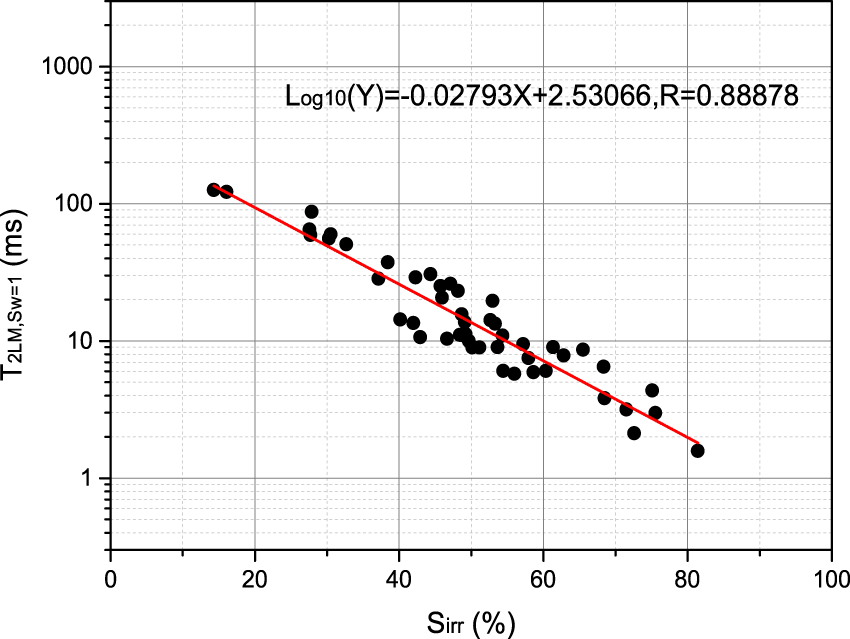
Figure 5. Parameter $T_{2LM,sw=1}$ as a function of the irreducible water saturation (S_irr).

Figure 5 shows the relationship model Equation 20, for which the goodness of fit is 0.88878.

The NMR experimental data from the 18 sealed sandstone samples were used to validate the oil saturation versus T2 geometric mean time relationship model (Equation 7). Using Equation 7 and Equation 10, the relationship between the experimental oil saturation $S_{oh}$ and $Lo{g}_{10}\left(\frac{T_{2LM}}{T_{2LM,SW=1}}\right)$ is determined, as shown in Figure 6. The corresponding relationship model is

$S_{oh}=1.2038Lo{g}_{10}\left(\frac{T_{2LM}}{T_{2LM,SW=1}}\right).(21)$

Figure 6

Figure 6. Relationship between the experimental oil saturation value and $Lo{g}_{10}\left(\frac{T_{2LM}}{T_{2LM,SW=1}}\right)$.

The goodness of fit for this model Equation 21 is R = 0.92014, and the results show that the coefficient k is approximately 1.2038 in the study area.

3.2 Case analyses in high- and low-resistivity-contrast reservoirs

To validate the oil saturation estimation method integrating NMR and resistivity logging data, we conducted comparative analyses wells NPX49 (high-resistivity-contrast reservoir) and XX16 (low-resistivity-contrast reservoir) of the Dongying Formation in Nanpu Sag. The corresponding results are presented in Figures 7, 8, and the detailed acquisition parameters are provided in Table 3. Both wells were configured for the D9TWE3 NMR logging mode as follows: Group A: TW_l = 12.988 s, TE_s = 0.9 ms, and 500 echoes; Group B: TW_s = 1 s, TE_s = 0.9 ms, and 500 echoes; Group C: TW_c = 0.02 s, TE_c = 0.6 ms, and 20 echoes; Group D: TW_l = 12.988 s, TE_l = 3.6 ms, and 125 echoes; Group E: TW_s = 1 s, TE_l = 3.6 ms, and 125 echoes.

Figure 7

Figure 7. Application of the proposed method to well NPX49 (layers 1–4).

Figure 8

Figure 8. Application of the proposed method to well XX16 (layers 1 and 2).

Table 3

Table 3. Reservoir parameters.

In Figures 7, 8, the tracks 1–12 include conventional well logs, dual-TE T2 spectra, NMR-logging-based clay-bound water saturation, NMR-logging-based capillary-bound water saturation, NMR-logging-based movable water saturation, NMR-logging-based permeability, T2 geometric mean time, calculated oil saturation of the invaded zone from NMR logging, calculated irreducible water saturation from NMR logging, calculated oil saturation of the uninvaded zone by the proposed method, and calculated water saturation of the uninvaded zone by the Archie equation and layer number.

Figure 7 presents the application results for well NPX49 (layers 1–4). The distributions of both long-TE and short-TE T2 spectra narrow progressively from layers 1 to 4. Both the resistivity logging and NMR T2 spectra indicate gradual decrease in oil saturation from layers 1 to 4. In layer 1, the clay content (0.04 v/v) has negligible influence on the measured resistivity. The calculated errors are less than 2% between the results of the experimental oil saturation and proposed methods as well as the experimental oil saturation method and Archie model. This demonstrates that both the proposed method and Archie model can accurately determine oil saturation in conventional reservoirs. Layer 1 exhibits a daily oil production of 14 m³ with no water production.

Figure 8 shows the application results for well XX16 (layers 1–3). The drilling mud resistivity was 0.15 Ω·m at 18°C, and the regional parameters were n = 1.78, $mi$ = 1.66, $mc=2$, ${\sigma }_{wf}=1.67\mathrm{S}/\mathrm{m}$, ${\sigma }_{wi}=1.67\mathrm{S}/\mathrm{m}$, and ${\sigma }_{wc}=4\mathrm{S}/\mathrm{m}$, as well as ${\sigma }_{mf}$ that was calculated based on the mud resistivity, reservoir depth, and geothermal gradient. It is seen that the distributions of the long-TE and short-TE T2 spectra of layer 1 have wide ranges, indicating the presence of oil; the corresponding distributions for layer 2 have narrow ranges, indicating the absence of oil. The calculated oil saturation values of layers 1 and 2 based on the new method are in good agreement with the experimental oil saturation values (errors less than 3%). Figure 9 shows a thin-section micrograph of layer 1 in well XX16 depicting that the I/S mixed layer has filled intergranular pores. As the high cation exchange capacity (Qv) caused by the high content of the I/S mixed layer cannot be accurately characterized by the Archie model, the oil saturation value calculated using the Archie model is contrary to the reservoir oiliness. The daily oil production of layer 1 is 8 m³ without water.

Figure 9

Figure 9. Thin-section micrograph of layer 1 from well XX16 (I/S: illite/smectite mixed layer) showing (A) I/S mixed layer filling in the intergranular pores and (B) I/S mixed layer on the granular surface.

In Figures 7, 8, the tracks from left to right are as follows: tracks 1–4: natural gamma-ray logging (GR: GAPI)/spontaneous potential logging (SP:MV), depth (m), apparent resistivity logs (RLLD/RLLS: Ω·m), acoustic wave slowness logs (AC: µs/m)/bulk density (DEN: g/cm³)/neutron porosity (CNL: %); track 5: NMR logging T2 spectra measured with parameters TE = 0.9 ms and TW = 12,988 ms (NMR.TA: ms); track 6: NMR logging T2 spectra measured with parameters TE = 3.6 ms and TW = 12,988 ms (NMR.TB: ms); track 7: clay-bound water saturation computed from NMR logging (PWC: v/v)/capillary-bound water saturation computed from NMR logging (PWI: v/v)/movable water saturation (POR: v/v) computed from NMR logging/experimental porosity of the rock samples (CORE.POR: v/v); track 8: permeability calculated from NMR logging (NMR.PERM: mD)/experimental permeability of the rock samples (CORE.PERM: mD); track 9: T2 geometric mean time of NMR.TA (T_2LM: ms)/T2 geometric mean time of the water-saturated rock (T_2LM,sw: ms); track 10: oil saturation of the invaded zone computed by NMR (SOH: v/v)/irreducible water saturation of the invaded zone computed by NMR (SWIR: v/v)/experimental irreducible water saturation of the rock samples (CORE.SWIR: v/v); track 11: Archie-model-based water saturation of the uninvaded zone (ARCHIE.SW: v/v)/experimental oil saturation of the rock samples (CORE.SO: v/v); track 12: oil saturation of the uninvaded zone calculated using the new method (NEW.SO: v/v)/experimental oil saturation of the rock samples (CORE.SO: v/v); track 13: layer number.

4 Discussion and future work

4.1 Factor analysis causing low-resistivity-contrast reservoir

Figure 7 shows a resistivity ratio of 3.7 (Ω·m/Ω·m) between layers 1 (oil layer) and 4 (water layer), indicating a high-resistivity-contrast reservoir, with the clay volume of layer 1 in Figure 7 being 0.02 v/v. Figure 8 demonstrates a resistivity ratio of 0.75 (Ω·m/Ω·m) between layers 1 (oil layer) and 2 (water layer), characteristic of a low-resistivity-contrast reservoir, with the clay volume of layer 1 in Figure 8 being 0.12 v/v.

Due Owing to the extremely high Qv of the montmorillonite and I/S mixed layer, as documented in Table 4, the rock resistivity is lower than those observed in conventional reservoirs with equivalent oil saturation. Figure 10A illustrates the experimental relationship between Qv and resistance increase rate. Figure 10B demonstrates the correlation between Qv and clay content. Figure 10C quantifies the relationship between Qv and the combined content of the montmorillonite and I/S mixed layer. Collectively, Figure 10 reveals (1) an inverse proportionality between the resistance increase rate and Qv as well as (2) a direct proportionality between the clay content and Qv, particularly for the montmorillonite and I/S mixed layer. This indicates that the low resistivity-contrast in the study area is a result of the high contents of montmorillonite and the I/S mixed layer minerals (Saidian et al., 2016).

Table 4

Table 4. Experimental cation exchange capacities of clay minerals.

Figure 10

Figure 10. Experimental relationships among Qv, resistance increase rate, clay content, and combined content of montmorillonite and I/S mixed layer. (A) Experimental relationship between Qv and resistance increase rate. (B) Experimental relationship between Qv and clay content. (C) Experimental relationship between Qv and combined content of montmorillonite and I/S mixed layer.

4.2 Factor analysis causing the calculation errors

The application results reveal that the oil saturation values calculated by the new method show good agreement with those from the Archie model in conventional reservoirs; furthermore, the new method provides more accurate oil saturation calculations than the Archie model in low-resistivity-contrast reservoirs. This difference is attributable to two key factors. First, compared with conventional reservoirs, low-resistivity-contrast reservoirs exhibit wider variation ranges for both formation factor and resistivity index under the Archie model (Al Gathe, 2009); in the proposed model, the value of the formation factor m has been eliminated, thereby eliminating its influence on the oil saturation calculation caused by the wide range of formation factors in low-resistivity-contrast oil layers. Second, the complex pore structures and mineral compositions in low-resistivity-contrast reservoirs reduce the sensitivity of the resistivity-log responses to pore fluids, consequently decreasing the calculation accuracy of the Archie model. Although a larger number of parameters are required by the proposed method than the Archie model, in addition to its greater complexity in practical applications, the new method effectively overcomes the problem of calculation errors in low-contrast reservoirs caused by the Archie model.

In Figure 7, at the middle depth of layers 1–4, the oil saturation calculated by the new method is consistent with that obtained with the Archie model. However, at the upper and lower edge depths of the reservoir, the curve-shaped results produced by the new method and Archie model are quite different; the depth distribution range of oil saturation calculated using the new method is wider, while that of the Archie model is narrower. This is attributable to the fact that when a sandstone reservoir approaches the upper and lower surrounding rocks (shale), the clay volume usually increases and eventually graduates into shale. An increase in clay volume usually leads to a decrease in the value of the formation factor m; in the Archie model, the formation factor m has a fixed value, which results in a rapid decrease in the calculated oil saturation and a narrow depth distribution range of the result. However, the proposed method eliminates the influence of the formation factor m such that the calculation result is more reasonable.

The sources of calculation errors in the proposed method may be as follows: ① Errors from the regional parameters determined using the experimental data, such as n, $mi$, $mc$, and k. ② Environmental effects on the log data. ③ Errors from invaded oil saturation calculated via NMR logging. ④ Errors caused by the step response model when simulating actual mud invasion.

4.3 Further research

The future research directions and topics concerning the new method for calculating oil saturation are as follows:

a. Oil saturation calculated with the new method can be used in further studies on low-resistivity-contrast reservoirs, such as reservoir assessment and estimation (Yang et al., 2013; Xie et al., 2020).

b. The invasion model of the mud filtrate can be improved to increase the calculation accuracy.

c. Dielectric logging may be an option for obtaining the oil saturation of the invaded zone (Amirmoshiri et al., 2018; Piedrahita and Aguilera, 2017; Freedman et al., 1997).

d. The oil saturation calculated with the new method can be further used to correct the oil content in capillary pressure conversion via the NMR T2 spectrum (Xie et al., 2021; Hosseinzadeh et al., 2020).

5 Conclusion

In this study, we focused on a new method of determining oil saturation by combining NMR logging and resistivity logging as well as its application to low-resistivity-contrast reservoirs. The main conclusions of this study are as follows:

1. The new method comprises two parts. First, the oil saturation of the invaded zone can be obtained by NMR analysis. Then, the oil saturation of the uninvaded zone can be calculated by further inversion according to the resistivity model.

2. In high-porosity and high-permeability reservoirs, the theoretical derivations and core sample verifications confirm that under a similar sedimentary environment, oil saturation is linearly related to $Lo{g}_{10}\left(\frac{T_{2LM,SW=1}}{T_{2LM,Swi}}\right)$ and that the irreducible water saturation is linearly related to $T_{2LM,SW=1}$. These observations provide a theoretical basis for estimating the oil saturation of the invaded zone based on NMR logging data.

3. Application results to real-world wells show that the oil saturation calculated by the new method is in good agreement with the production test and that the accuracy is higher than that calculated by the Archie model for low-resistivity-contrast reservoirs.

4. The oil saturation calculation method proposed in this work can be effectively utilized to compute the reservoir parameters, thereby contributing positively to the exploration and identification of special oil and gas reservoirs.

Data availability statement

The raw data supporting the conclusions of this article will be made available by the authors, without undue reservation.

Author contributions

WX: writing – original draft, investigation, methodology, writing – review and editing. QY: methodology, formal analysis, writing – original draft, writing – review and editing. YL: writing – review and editing, methodology. XD: formal analysis, writing – review and editing. JZ: data curation, writing – review and editing, formal analysis. PZ: formal analysis, writing – review and editing.

Funding

The author(s) declare that financial support was received for the research and/or publication of this article. This article was supported by the Research Foundation of Karamay, China (no. 2024hjcxrc0075), Key Research and Development Program Project of Xinjiang (nos. 2024B01016, 2024B01016-1, and 2024B01016-3), Research Foundation of the China University of Petroleum-Beijing at Karamay (no. XQZX20230012), “Tianchi Talent” Introduction Plan Foundation of Xinjiang, and Natural Science Foundation of Xinjiang (no. 2021D01E22).

Conflict of interest

Author YL was employed by Xinjiang Oilfield Company of PetroChina.

Author JZ was employed by China Petroleum Logging Co., Ltd.

The remaining authors declare that the research was conducted in the absence of any commercial or financial relationships that could be construed as a potential conflict of interest.

Generative AI statement

The author(s) declare that no Generative AI was used in the creation of this manuscript.

Publisher’s note

All claims expressed in this article are solely those of the authors and do not necessarily represent those of their affiliated organizations, or those of the publisher, the editors and the reviewers. Any product that may be evaluated in this article, or claim that may be made by its manufacturer, is not guaranteed or endorsed by the publisher.

References

Al-Gathe, A. (2009). “Analysis of archie's parameters determination techniques,” in M.Sc thesis. King Fahd University of Petroleum and Minerals. Saudi Arabia.

Google Scholar

Amirmoshiri, M., Zeng, Y., Chen, Z., Singer, P. M., Puerto, M. C., Grier, H., et al. (2018). Probing the effect of oil type and saturation on foam flow in porous media: core-flooding and nuclear magnetic resonance (NMR) imaging. Energy Fuels 32 (11), 11177–11189. doi:10.1021/acs.energyfuels.8b02157

CrossRef Full Text | Google Scholar

Arbab, B., Jahani, D., and Movahed, B. (2017). Reservoir characterization of carbonate in low resistivity pays zones in the buwaib formation, Persian Gulf. Open J. Geol. 7 (09), 1441–1451. doi:10.4236/ojg.2017.79096

CrossRef Full Text | Google Scholar

Archie, G. E. (1942). The electrical resistivity log as an aid in determining some reservoir characteristics. Trans. AIME 146 (01), 54–62. doi:10.2118/942054-g

CrossRef Full Text | Google Scholar

Bashiri, M., Kamari, M., and Zargar, G. (2017). An Improvement in cation exchange capacity estimation and water saturation calculation in shaly layers for one of Iranian oil fields. Iran. J. Oil Gas Sci. Technol. 6 (1), 45–62. doi:10.22050/ijogst.2017.44376

CrossRef Full Text | Google Scholar

Liang, B., Jiang, H., Li, J., Gong, C., Jiang, R., Qu, S., et al. (2017). Investigation of oil saturation development behind spontaneous imbibition front using nuclear magnetic resonance T2. Energy Fuels 31 (1), 473–481. doi:10.1021/acs.energyfuels.6b02903

CrossRef Full Text | Google Scholar

Boaca, T., and Boaca, I. (2018). A nonlinear single phase mud-filtrate invasion model. J. Petrol. Sci. Eng. 168, 39–47. doi:10.1016/j.petrol.2018.05.007

CrossRef Full Text | Google Scholar

Chatterjee, R., Gupta, S. D., and Farooqui, M. Y. (2012). Application of nuclear magnetic resonance logs for evaluating low resistivity reservoirs: a case study from the cambay basin, India. J. Geophys. Eng. 9 (5), 595–610. doi:10.1088/1742-2132/9/5/595

CrossRef Full Text | Google Scholar

Chen, L., Zou, C., Wang, Z., Liu, H., Yao, S., and Chen, D. (2009). Logging evaluation method of low resistivity reservoir—a case study of well block DX12 in Junggar basin. J. Earth Sci. 20 (06), 1003–1011. doi:10.1007/s12583-009-0086-0

CrossRef Full Text | Google Scholar

Chen, C., Pan, B., Lin, X., Zhang, P., Zhang, L., Ren, S., et al. (2025). Evaluation of low-resistivity reservoirs based on the new three-water model and comprehensive identification of fluid properties using a committee machine—a case study of the Dongying Formation Member 1 Reservoir in the Gangdong Fault Zone. J. Geophys. Eng. 22 (2), 532–543. doi:10.1093/jge/gxaf022

CrossRef Full Text | Google Scholar

Clavier, C., Coates, G., and Dumanoir, J. (1984). Theoretical and experimental bases for the dual-water model for interpretation of shaly sands. Soc. Petr. Eng. J. 24 (02), 153–168. doi:10.2118/6859-PA

CrossRef Full Text | Google Scholar

Feng, C., Gingras, M., Sun, M., and Wang, B. (2017). Logging characteristics and identification methods of low resistivity oil layer: Upper Cretaceous of the third member of Qingshankou Formation, Daqingzijing Area, Songliao Basin, China. Geofluids, 2915646. doi:10.1155/2017/2915646

CrossRef Full Text | Google Scholar

Freedman, R. (2006). Advances in NMR logging. J. Petrol. Technol. 58 (01), 60–66. doi:10.2118/89177-JPT

CrossRef Full Text | Google Scholar

Freedman, R., Johnston, M., Morriss, C. E., Straley, C., Tutunjian, P. N., and Vinegar, H. J. (1997). Hydrocarbon saturation and viscosity estimation from NMR logging in the Belridge Diatomite. Log Analyst 38 (02). Available online at: https://onepetro.org/petrophysics/article-abstract/170904/Hydrocarbon-Saturation-And-Viscosity-Estimation.

Google Scholar

Fordham, E. J., Kenyon, W. E., Ramakrishnan, T. S., Schwartz, L. M., and Wilkinson, D. J. (1999). Forward models for nuclear magnetic resonance in carbonate rocks. Log Analyst 40 (4), 260–270. Available online at: https://onepetro.org/petrophysics/article-abstract/170963/Forward-Models-For-Nuclear-Magnetic-Resonance-In.

Google Scholar

Ge, X., Mao, G., Hu, S., Li, J., Zuo, F., Zhang, R., et al. (2023). Laboratory NMR study to quantify the water saturation of partially saturated porous rocks. Lithosphere 2023, 1214083. doi:10.2113/2023/1214083

CrossRef Full Text | Google Scholar

George, C., Xiao, L. Z., and Manfred, P. (2007). Principle and application of nuclear magnetic resonance logging. Beijing, China. Petroleum Industry Press.

Google Scholar

Gong, H., Zhu, C., Zhang, Y., Li, Z., San, Q., Xu, L., et al. (2020). Experimental evaluation on the oil saturation and movability in the organic and inorganic matter of shale. Energy Fuels 34 (7), 8063–8073. doi:10.1021/acs.energyfuels.0c00831

CrossRef Full Text | Google Scholar

Gunawan, A. Y., Sukarno, P., and Soewono, E. (2011). Modeling of mud filtrate invasion and damage zone formation. J. Petrol. Sci. Eng. 77 (3-4), 359–364. doi:10.1016/j.petrol.2011.04.011

CrossRef Full Text | Google Scholar

Heaton, N. J., Minh, C. C., Kovats, J., and Guru, U. (2004). “Saturation and viscosity from multidimensional nuclear magnetic resonance logging,” in SPE Annual Technical Conference and Exhibition. (Houston, TX: Society of Petroleum Engineers). doi:10.2118/90564-MS

CrossRef Full Text | Google Scholar

Hodgkins, M. A., and Howard, J. J. (1999). Application of NMR logging to reservoir characterization of low-resistivity sands in the Gulf of Mexico. AAPG Bull. 83 (1), 114–127. doi:10.1306/00AA9A16-1730-11D7-8645000102C1865D

CrossRef Full Text | Google Scholar

Hosseinzadeh, S., Kadkhodaie, A., and Yarmohammadi, S. (2020). NMR derived capillary pressure and relative permeability curves as an aid in rock typing of carbonate reservoirs. J. Petrol. Sci. Eng. 184, 106593. doi:10.1016/j.petrol.2019.106593

CrossRef Full Text | Google Scholar

Hu, X., Cheng, R., Zhang, H., Zhu, J., Chi, P., and Sun, J. (2024). Three-water differential Parallel conductivity saturation model of low-permeability tight oil and gas reservoirs. Energies 17 (7), 1726. doi:10.3390/en17071726

CrossRef Full Text | Google Scholar

Iqbal, M. A., Salim, A. M. A., Baioumy, H., Gaafar, G. R., and Wahid, A. (2019). Identification and characterization of low resistivity low contrast zones in a clastic outcrop from Sarawak, Malaysia. J. Appl. Geophys. 160, 207–217. doi:10.1016/j.jappgeo.2018.11.013

CrossRef Full Text | Google Scholar

Jianmin, W., and San, Z. (2018). Pore structure differences of the extra-low permeability sandstone reservoirs and the causes of low resistivity oil layers: a case study of Block Yanwumao in the middle of Ordos Basin, NW China. Petrol. Explor. Dev. 45 (02), 273–280. doi:10.1016/S1876-3804(18)30030-2

CrossRef Full Text | Google Scholar

Kurniawan, F. (2005). Shaly sand interpretation using CEC-dependent petrophysical parameters. LA, United States: Louisiana State University. Ph.D.Thesis. doi:10.31390/gradschool_dissertations.2384

CrossRef Full Text | Google Scholar

Lai, J., Pang, X., Xu, F., Wang, G., Fan, X., Xie, W., et al. (2019). Origin and formation mechanisms of low oil saturation reservoirs in Nanpu Sag, Bohai Bay Basin, China. Mar. Petrol. Geol. 110, 317–334. doi:10.1016/j.marpetgeo.2019.07.021

CrossRef Full Text | Google Scholar

Li, C., Shi, Y., Zhou, C., Li, X., Liu, B., Tang, L., et al. (2010). Evaluation of low amplitude and low resistivity pay zones under the fresh drilling mud invasion condition. Petrol. Explor. Dev. 37 (6), 696–702. doi:10.1016/S1876-3804(11)60004-9

CrossRef Full Text | Google Scholar

Liu, X. P., Hu, X. X., Zhang, X. L., Xu, R., and Zhi, L. L. (2013). Applications of conventional logs in low resistivity contrast tight gas reservoirs identification. Adv. Mater. Res. 734-737, 41–44. doi:10.4028/www.scientific.net/AMR.734-737.41

CrossRef Full Text | Google Scholar

Li, C. X., Liu, M., and Guo, B. C. (2019). Classification of tight sandstone reservoirs based on NMR logging. Appl. Geophys. 16 (4), 549–558. doi:10.1007/s11770-019-0793-y

CrossRef Full Text | Google Scholar

Liu, B., Yang, Y., Li, J., Chi, Y., Li, J., and Fu, X. (2020). Stress sensitivity of tight reservoirs and its effect on oil saturation: a case study of Lower Cretaceous tight clastic reservoirs in the Hailar Basin, Northeast China. J. Petrol. Sci. Eng. 184, 106484. doi:10.1016/j.petrol.2019.106484

CrossRef Full Text | Google Scholar

Lubis, L. A., Ghosh, D. P., and Hermana, M. (2016). Elastic and electrical properties evaluation of low resistivity pays in Malay basin clastics reservoirs. IOP Conf. Ser. Earth Environ. Sci. 38, 012004. doi:10.1088/1755-1315/38/1/012004

CrossRef Full Text | Google Scholar

Mannhardt, K., and Svorstøl, I. (1999). Effect of oil saturation on foam propagation in Snorre reservoir core. J. Petrol. Sci. Eng. 23 (3-4), 189–200. doi:10.1016/S0920-4105(99)00016-9

CrossRef Full Text | Google Scholar

Mashaba, V., and Altermann, W. (2015). Calculation of water saturation in low resistivity gas reservoirs and pay-zones of the Cretaceous Grudja Formation, onshore Mozambique basin. Mar. Petrol. Geol. 67, 249–261. doi:10.1016/j.marpetgeo.2015.05.016

CrossRef Full Text | Google Scholar

Piedrahita, J., and Aguilera, R. (2017). “Estimating oil saturation index OSI from NMR logging and comparison with Rock-Eval pyrolysis measurements in a Shale oil reservoir,” in SPE Unconventional Resources Conference (Calgary, Alberta, CA:Society of Petroleum Engineers). doi:10.2118/185073-MS

CrossRef Full Text | Google Scholar

Pratama, E., Suhaili Ismail, M., and Ridha, S. (2017). An integrated workflow to characterize and evaluate low resistivity pay and its phenomenon in a sandstone reservoir. J. Geophys. Eng. 14 (3), 513–519. doi:10.1088/1742-2140/aa5efb

CrossRef Full Text | Google Scholar

Qin, Z., Hou, M., Wang, Z. H., Guo, M. C., and Liu, R. (2013). Logging fluid identification method of low resistivity contrast reservoir invaded by fresh water mud —a case study of well block YD in Erdos Basin. Appl. Mech. Mater. 318, 442–446. doi:10.4028/www.scientific.net/AMM.318.442

CrossRef Full Text | Google Scholar

Rios, E., Figueiredo, I., Muhammad, A., Azeredo, R. B. D. V., and Glassborow, B. (2014). “NMR permeability Estimators under different relaxation time Selections: a Laboratory study of cretaceous Diagenetic Chalks,” in SPWLA 55th Annual Logging Symposium, 18–22. Available online at: https://onepetro.org/SPWLAALS/proceedings-abstract/SPWLA14/All-SPWLA14/28366.

Google Scholar

Saidian, M., Godinez, L. J., and Prasad, M. (2016). Effect of clay and organic matter on nitrogen adsorption specific surface area and cation exchange capacity in shales (mudrocks). J. Nat. Gas Sci. Eng. 33, 1095–1106. doi:10.1016/j.jngse.2016.05.064

CrossRef Full Text | Google Scholar

Shang, B. Z., Hamman, J. G., and Caldwell, D. H. (2004). “A physical model to explain the First Archie Re1ationship and beyond,” in SPE Annual Technical Conference and ExhIbition. Denver, Colorado: U S A. doi:10.2118/84300-MS

CrossRef Full Text | Google Scholar

Song, F., Xiao, C. W., Bian, S. T., Xiao-Jun, S. U., and Wang, H. Z. (2008). Origin of low resistivity reservoirs in low angle drape structure in lunnan, tarim basin. Petrol. Explor. Dev. 35 (1), 108–112. doi:10.1016/S1876-3804(08)60015-4

CrossRef Full Text | Google Scholar

Wang, X., Wang, Z., Feng, C., Zhu, T., Zhang, N., Feng, Z., et al. (2019). Predicting oil saturation of tight conglomerate reservoirs via well logs based on reconstructing nuclear magnetic resonance T2 spectrum under completely watered conditions. J. Geophys. Eng. 17 (2), 328–338. doi:10.1093/jge/gxz109

CrossRef Full Text | Google Scholar

Waxman, M. H., and Thomas, E. C. (1974). Electrical conductivities in shaly sands-i. the relation between hydrocarbon saturation and resistivity index; ii. the temperature coefficient of electrical conductivity. J. Petrol. Technol. doi:10.2118/4094-MS

CrossRef Full Text | Google Scholar

Xie, W., Yin, Q., Wang, G., Guan, W., and Yu, Z. (2021). Modeling and evaluation method of gas saturation based on P-wave and pore structure classification in low porosity and low permeability reservoir. Arabian J. Geosci. 14, 917. doi:10.1007/s12517-021-07331-9

CrossRef Full Text | Google Scholar

Xie, W., Yin, Q., Wang, G., and Yu, Z. (2020). Variable Dimension Fractal-based conversion method between the nuclear magnetic resonance T2 spectrum and capillary pressure curve. Energy Fuels 35 (1), 351–357. doi:10.1021/acs.energyfuels.0c02924

CrossRef Full Text | Google Scholar

Xu, C., and Torres-Verdín, C. (2013). Pore system characterization and petrophysical rock classification using a bimodal Gaussian density function. Math. Geosci. 45 (6), 753–771. doi:10.1007/s11004-013-9473-2

CrossRef Full Text | Google Scholar

Christensen, S. A., Holger, F. T., and Ole, V. (2015). “NMR fluid substitution method for reservoir characterization and drilling optimization in low-porosity chalk,” in SPWLA 56th Annual Logging Symposium, 18–22. Available online at: https://onepetro.org/SPWLAALS/proceedings-abstract/SPWLA15/SPWLA15/28508.

Google Scholar

Xu, C., Misra, S., Srinivasan, P., and Ma, S. (2019). “When petrophysics meets big data: what can machine do?,” in SPE Middle East Oil and Gas Show and Conference (Manama, Bahrain: Society of Petroleum Engineers). doi:10.2118/195068-MS

CrossRef Full Text | Google Scholar

Yan, X., Zhu, Z., and Wu, Q. (2018). Intelligent inversion method for pre-stack seismic big data based on MapReduce. Comput. Geosci. 110, 81–89. doi:10.1016/j.cageo.2017.10.002

CrossRef Full Text | Google Scholar

Yang, P., Guo, H., and Yang, D. (2013). Determination of residual oil distribution during waterflooding in tight oil formations with NMR relaxometry measurements. Energy Fuels 27 (10), 5750–5756. doi:10.1021/ef400631h

CrossRef Full Text | Google Scholar

Zhang, M. L., Liu, C. L., Li, Y., and Wu, J. Y. (2013). Geological characteristics of difficult reservoirs in logging interpretation. Adv. Mater. Res. 616-618, 151–157. doi:10.4028/www.scientific.net/AMR.616-618.151

CrossRef Full Text | Google Scholar

Glossary

$T_{2LM}$ T2 geometric mean time of oil-bearing rock

$T_{2LM,sw=1}$ T2 geometric mean time of water-saturated rock

$T_{2LM,oil}$ T2 geometric mean time of oil spectrum

$T_{2LM,wf}$ T2 geometric mean time of free water spectrum in oil-bearing rock

$T_{2LM,wm}$ T2 geometric mean time of free water spectrum in water-saturated rock

$T_{2LM,wi}$ T2 geometric mean time of irreducible water spectrum

${\varphi }_{i,wi}$ Irreducible water porosity of pore component i

${\varphi }_{i,o}$ Oil porosity of pore component i

${\varphi }_{i,wf}$ Free water porosity of pore component i

${\varphi }_t$ Total porosity

$T_{2,i}$ T2 value of pore component i

${\varphi }_{i,wf}$ Free water porosity of pore component i in water-saturated rock

${\varphi }_{oil}$ Pore volume of oil

$S_{oh}$ Oil saturation of invaded zone

$S_{wf}$ Free water saturation

$S_{wi}$ Irreducible water saturation

$S_o$ Oil saturation in uninvaded zone

$F_{wf}$ Formation factor of free water

$F_{wi}$ Capillary irreducible water

$F_{wc}$ Clay-bound water

${\sigma }_t$ Measured conductivity of uninvaded zone

${\varphi }_f$ Porosity of movable fluids

${\varphi }_{wi}$ Porosity of capillary irreducible water

${\varphi }_{wc}$ Porosity of clay irreducible water

$\mathrm{N}$ Saturation factor

$mf$ Cementation factor of movable water

$mi$ Cementation factor of capillary irreducible water

$mc$ Cementation factor of clay irreducible water

${\sigma }_{wf}$ Conductivity of movable water

${\sigma }_{wi}$ Conductivity of capillary irreducible water

${\sigma }_{wc}$ Conductivity of clay irreducible water

${\sigma }_{mf}$ Conductivity of mud filtrate

$d{\sigma }_t$ Differential of ${\sigma }_t$

$d{\sigma }_{wf}$ Differential of ${\sigma }_{wf}$