Deep learning driven reconstruction of acoustic logging signal in energy exploration and development

In oil and gas exploration and development, logging curves are the key data for obtaining underground geological information. However, in actual acquisition processes, problems such as drilling fluid invasion and wellbore collapse often lead to the absence or distortion of logging data, thereby affecting their subsequent analysis and application. Well logging curves exhibit clear context-dependent characteristics. Traditional reconstruction methods are mostly based on the assumption of independent and identically distributed data and are difficult to capture the temporal dependencies between data, resulting in limited accuracy of time series modeling. Therefore, for the shale reservoir in a certain basin in the northeastern region, this paper introduces a method that combines variational mode decomposition (VMD), convolutional neural network (CNN), and bidirectional long short-term memory neural network (BiLSTM) to achieve high-precision reconstruction of logging acoustic wave signals (DT). The VMD method decomposes the logging curves into different mode functions (IMF), achieving the extraction of features at different scales; the CNN method is used to extract local features such as local morphology and change trends of IMF, obtaining high-level feature representations; the BiLSTM is used to extract the bidirectional long-term dependencies of features. By standardizing the logging data, to avoid the subjectivity of manually selecting the input logging curves, the XGBoost-SHAP method is introduced to optimize the logging curves, and an DT-targeted gradient boosting regression model is constructed using XGBoost, and the SHAP values are used to conduct game theory-based contribution analysis for each input feature, obtaining the feature ranking based on the cumulative SHAP contribution. Finally, three sensitive curves, CNL, GR, and RS, are selected as input features to construct the VMD-CNN-BiLSTM prediction model, which is applied to two test wells, achieving a fitting goodness (R²) of 0.71 and 0.88 respectively. Further comparative experiments have shown that the VMD-CNN-BiLSTM model has significantly improved performance in terms of MSE, MAE, MAPE, R², etc., compared to the SVR, random forest, and LSTM methods. The MSE has increased by 20.5–33.9, MAE by 1.5–2.1, MAPE by 1.6%–2.3%, and R² by 0.21–0.36.

1 Introduction

In petroleum exploration, logging curves constitute essential geological data that facilitate for-mation evaluation through lithology interpretation, reservoir parameter determination, and seismic inversion processes. Among them, the acoustic logging curves directly reflect the coupling effect of the elastic modulus of the rock matrix and the compressibility of the pore fluids by recording the propagation time of the longitudinal waves in the formation. They are mainly used in synthetic seismic records, lithology discrimination, porosity calculation, and rock mechanics parameter calculation. In the actual logging process, interference from unfavorable factors such as borehole collapse and instrument failure can lead to problems such as missing data and distortion of logging curves (Wang et al., 2020), which increases the difficulty of subsequent geological work. In view of the high cost of re-logging, engineering difficulty and other problems (Zhou et al., 2022), how to carry out logging curve re-construction has become a key link in the exploration and development of oil and gas reservoirs.

To solve this problem, early researchers mainly used traditional methods for curve reconstruc-tion, such as empirical formulas (Chen and Wang, 2005; Yuan et al., 2009), petrophysical modeling (Li et al., 2016; Zhao et al., 2016), and multiple regression (Yin et al., 2014; Liao, 2014; Wang et al., 2016). However, in complex geological formations, logging curves often exhibit intricate nonlinear correla-tions. Conventional methods fail to adequately characterize these relationships, leading to poor re-construction accuracy that falls short of practical application standards.

With the development and application of machine learning, relevant algorithms have been widely used in the petroleum field. Machine learning algorithms such as K nearest neighbor (Aftab et al., 2023), support vector machine, random forest (Ibrahim and Elkatatny, 2022), and XGBoost (Zhang et al., 2022) have been widely used in relevant research. These algorithms are able to mine the complex nonlinear relationship between data, which improves the reconstruction accuracy to a certain extent. However, the “point-by-point prediction” paradigm has a fundamental flaw: they treat time series as independent and identically distributed observation points, thereby destroying the inherent temporal continuity. For instance, KNN only relies on numerical similarity and ignores the context order, making it prone to finding incorrect historical similar points; Random Forest, through bootstrap sampling and random feature selection, disrupts the temporal order, and its model structure cannot jointly maintain or remember long-term temporal states. Therefore, these methods are difficult to systematically capture time dependence (Zhou et al., 2025).

Deep learning, as an important branch of machine learning, provides a new solution for the re-construction of logging curves (Zhan et al., 2024; Liu D. et al., 2024). Deep learning models represented by convolutional neural network (CNN) (Zhai et al., 2023; Gama et al., 2025; Li et al., 2023) and recurrent neural network (RNN, LSTM) (Zhang et al., 2024; Liu J. et al., 2024; Shang et al., 2022) have been widely introduced into this field. CNN can effectively extract the spatial features of the logging data and explore the correla-tion between different parameters; RNN and its variants are good at dealing with the time-series da-ta and capture the information of the logging curve changes with depth, which is suitable for the re-construction of logging curve.

We make the following key contributions in this paper:

1. We employed the XGBoost-SHAP method for interpretability-based feature selection. This method is capable of effectively extracting the nonlinear relationships between the feature variables and the target variable, and can also explore the influence of multi-variable interaction effects on the prediction outcome.

2. We employed a combined loss function that integrates the soft dynamic time warping loss (Soft-DTW) and the mean square error loss (MSE). The Soft-DTW is used to measure the global similarity of the predicted curve and the actual curve, while the MSE is used to measure the single-point error. The combination of these two losses is utilized to better balance the scatter error of the well logging curve points and the overall trend error.

3. We utilize VMD to decompose the input and target curves into multi-frequency components, build CNN-BiLSTM models for each component, and superimpose the predicted components to reconstruct the final curve.

The rest of the paper is organized as follows: Section 2 summarizes the previous work. Section 3 explains the principles of the algorithms involved. Section 4 involved data preprocessing, feature selection, sample construction, model training, application effect analysis, and comparison experiments. Section 5 concludes the work of this paper.

2 Related works

As fundamental datasets for subsurface characterization, the quality (completeness and preci-sion) of well logging curves directly impacts the reliability of reservoir assessment. Traditional em-pirical formulas and petrophysical modeling methods can make preliminary estimation of the curve based on statistical laws, but there are obvious limitations in reconstruction accuracy in the face of the nonlinear relationship between logging data and its obvious spatial sequence characteristics under complex geological conditions.

The application of machine learning algorithms brings a new technical path for logging curve reconstruction. Kim and Cho (2024) applied a K-nearest neighbor collaborative filtering interpolation method for missing logging completion in a district in Norway, which demonstrated that the collab-orative filtering method, which is mainly applied to recommender system, can be better used for the interpolation of missing well logging data. Zhang et al. (2022) found through comparative experiments that the XGBoost algorithm has better accuracy and stability in the task of logging curve reconstruc-tion, showing stronger generalization ability. Li and Jiang (2025) further analyzed the XGBoost-based acoustic logging curve reconstruction in combination with the SHAP algorithm, confirming that fea-ture importance is crucial for model prediction accuracy. Afifi and Anifowose (2023) investigated the effectiveness of artificial neural networks, regression trees, support vector machines, and random forests in predicting acoustic wave curves. Among them, random forests had the lowest error rate, and through different feature combinations, it was confirmed that only using cable logging data was sufficient to achieve high-precision predictions. Nero et al. (2023) employed the support vector machine (SVM), random forest (RF), and extreme gradient boosting (XGBoost) algorithms to predict the acoustic wave curves of the Tano basin of Ghana, and confirmed that the generalization ability of the integrated machine learning algorithms is superior to that of the non-integrated learning algorithms. Saleh et al. (2025) examined the effectiveness of six machine learning algorithms, including random forest, in predicting acoustic logging curves. They concluded that the accuracy of ensemble models such as random forest and XGBoost was the highest. Additionally, they emphasized that feature engineering is crucial for enhancing the performance of the models. Due to their architectural limitations, tradi-tional machine learning methods often fail to effectively model long-term temporal dependencies in datasets.

The rise of deep learning has revolutionized the new paradigm of logging curve reconstruction. Zhai et al. (2023) used a two-dimensional convolutional neural network (CNN) and introduced an at-tention mechanism to strengthen the deep learning network’s ability to capture the autocorrelation and inter-correlation feature information of logging curves, and verified the reconstruction results with high accuracy through synthetic seismic records. Zhang et al. (2024) used a two-way long-short-term network method optimized by a particle swarm algorithm for the reconstruction of The particle swarm method obtains reasonable hyperparameters for the network and reduces the uncertainty of manual parameter adjustment, and the model has the ability of dynamic optimization and adaptive reconstruction in the process of logging reconstruction, which is applied to Qinshui Ba-sin with good results. Qu et al. (2025) proposed an interpolation method based on generative adver-sarial network algorithm for the problem of incomplete logging data. The application results show that the proposed method can effectively extract spatio-temporal features and correlations from log-ging data, and has stable interpolation capability for logging data with different missing rates and missing locations.

This study proposes a novel hybrid VMD-CNN-BiLSTM model for acoustic time-series (DT) re-construction, with experimental results demonstrating its superior performance.

3 Deep learning method for well logging acoustic signal reconstruction

3.1 Variational modal decomposition (VMD)

Variational Mode Decomposition (VMD) was proposed by Dragomiretskiy and Zosso (2013). It is an adaptive signal processing method. Different from traditional signal processing methods based on Fourier transform or wavelet transform, VMD decomposes complex multi-component signals into multiple Intrinsic Mode Functions (IMFs) with different central frequencies. These IMFs have specific physical meanings and excellent properties, enabling the effective extraction of features from different frequency components in the signal. As a result, VMD has been widely applied in the field of signal processing. The VMD method seeks a set of mode functions through variational optimization. Its objective function aims to minimize the sum of the bandwidths of all IMFs, with the constraint that the sum of all IMFs is equal to the original signal. The formula is shown in Equations 1, 2:

${\mathit{f}}_{\mathit{min}}=\underset{\left\{{\mathit{u}}_{\mathit{k}}\right\},\left\{{\mathit{\omega }}_{\mathit{k}}\right\}}{\mathit{min}}\left\{{\displaystyle \sum _{\mathit{k}}}{\left|\mathit{\partial }\left(\mathit{t}\right)\left[\left(\mathit{\delta }\left(\mathit{t}\right)+\frac{\mathit{j}}{\mathit{\pi }\mathit{t}}\right)*{\mathit{u}}_{\mathit{k}}\left(\mathit{t}\right)\right]{\mathit{e}}^{-\mathit{j}{\mathit{\omega }}_{\mathit{k}}\mathit{t}}\right|}_2^2\right\}(1)$

$s.t{\displaystyle \sum _{\mathit{k}=1}^{\mathit{K}}}{\mathit{u}}_{\mathit{k}}=\mathit{f}\left(\mathit{t}\right)(2)$

Where $\mathrm{\delta }\left(t\right)$ is the Dirac function, ∗ denotes the convolution operation, $\partial \left(t\right)$ denotes the derivative with respect to time, j is the imaginary unit, and $f\left(t\right)$ is the original signal, decomposed into k modal functions $u_k\left(t\right)$, each of which corresponding to a center frequency ${\omega }_k$.

In this study, the VMD method is used to decompose the logging curve data into sub-series with different frequencies, which respond to the overall trend, and local change characteristics of the logging curve. The high complexity and strong nonlinear characteristics of this time series can be solved by this processing.

3.2 Convolutional neural network (CNN)

Convolutional Neural Networks (CNNs) represent a class of deep neural networks characterized by their convolutional operations, originally developed for and predominantly applied in computer vision tasks. The core idea of CNN is to utilize convolutional operation to achieve the extraction of local features (e.g., edges, textures). Through the stacking of multiple convolutional layers, CNN can gradually abstract from low-level features to high-level semantic features, realizing the hierarchical expression of data features. Compared with the traditional fully connected neural network, CNN significantly reduces the number of model parameters through the weight sharing strategy and effectively avoids the overfitting problem (Wu et al., 2024). In this study, the well logging curves are presented in a 1D sequence format, where each data point corresponds to a specific depth. The local correlation between adjacent depth points (such as the sudden signal change at the interface between sandstone and mudstone) directly reflects the subtle geological changes. The 1D-CNN is designed to scan the 1D well logging sequence using a 1D convolution kernel, thereby capturing local spatial features. This method is directly similar to the way two-dimensional convolutional neural networks capture textures and edges in images.

The core component of CNN is the convolutional layer, which generates feature maps through convolution operations (Figure 1). The input data passes through the convolution kernel, and the mathematical expression is shown in Equation 3:

$\mathit{Y}\left[\mathit{i},\mathit{j}\right]={\displaystyle \sum _{\mathit{m}=0}^{\mathit{M}-1}}{\displaystyle \sum _{\mathit{n}=0}^{\mathit{N}-1}}\mathit{X}\left[\mathit{i}+\mathit{m},\mathit{j}+\mathit{n}\right]·\mathit{W}\left[\mathit{m},\mathit{n}\right]+\mathit{b}(3)$

Figure 1

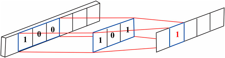
Figure 1. Schematic of 1D convolutional computation.

Where M × N denotes the convolution kernel size, W is the weight, and b is the bias term.

A conventional CNN framework typically comprises three fundamental components: (1) an input layer for raw image data reception, (2) a convolutional module containing sequentially arranged convolutional operations, nonlinear activation units, and downsampling layers for hierarchical feature extraction and dimensional reduction, and (3) a fully-connected classifier for final feature-to-label transformation.

3.3 Long short-term memory network (LSTM)

Long Short-Term Memory network (LSTM) is a special kind of Recurrent Neural Network (RNN) proposed by Hochreiter and Schmidhuber (1997), the core of which is to solve the problem of gradient vanishing and explosion encountered by RNN when dealing with long sequence data. Long Short-Term Memory (LSTM) networks are suitable for processing temporal data and are widely used in speech processing and natural language processing. LSTM controls the flow of information through three gate structures: forgetting gate, memorizing gate, and output gate (Figure 2).

Figure 2

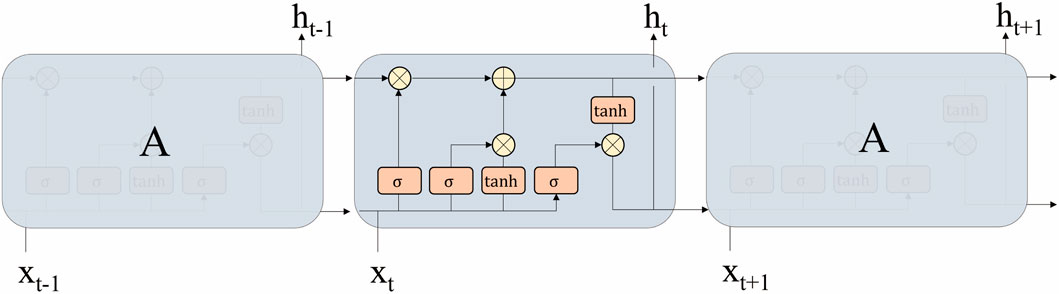
Figure 2. Structural diagram of the neural network for long short-term memory.

Oblivion Gate: selectively forgets historical information about the input. This component receives the information $h_{t-1}$ of the previous time state and the current input $x_t$, expressed as the formula is shown in Equation 4:

${\mathit{f}}_{\mathit{t}}=\mathit{\sigma }\left({\mathit{W}}_{\mathit{f}}·\left[{\mathit{h}}_{\mathit{t}-1},{\mathit{x}}_{\mathit{t}}\right]+{\mathit{b}}_{\mathit{f}}\right)(4)$

Where $f_t$ is the output information of the forgetting gate, $\sigma$ is the activation function, $W_f$ is the weight, and $b_f$ is the bias.

Input Gate: Controls the addition of current input information to the memory cell. The update of the information in the memory cell and the generation of a new memory value is controlled by an activation function, expressed by the formula is shown in Equations 5, 6:

${\mathit{i}}_{\mathit{t}}=\mathit{\sigma }\left({\mathit{W}}_{\mathit{i}}·\left[{\mathit{h}}_{\mathit{t}-1},{\mathit{x}}_{\mathit{t}}\right]+{\mathit{b}}_{\mathit{i}}\right)(5)$

$\stackrel{\sim }{{\mathit{C}}_{\mathit{t}}}=\mathit{tanh}\left({\mathit{W}}_{\mathit{C}}·\left[{\mathit{h}}_{\mathit{t}-1},{\mathit{x}}_{\mathit{t}}\right]+{\mathit{b}}_{\mathit{C}}\right)(6)$

Where $i_t$ is the output of the input gate, $\stackrel{\sim }{C_t}$ is the candidate memory value at the current moment, and $\mathit{tanh}$ is the activation function.

Output gate: the output gate selectively filters the composite information derived from both the memory cell state and current input features, thereby determining the final output representation and generating an updated hidden state through a gating mechanism, which is expressed by Equations 7, 8:

${\mathit{o}}_{\mathit{t}}=\mathit{\sigma }\left({\mathit{W}}_{\mathit{o}}·\left[{\mathit{h}}_{\mathit{t}-1},{\mathit{x}}_{\mathit{t}}\right]+{\mathit{b}}_{\mathit{o}}\right)(7)$

${\mathit{h}}_{\mathit{t}}={\mathit{o}}_{\mathit{t}}·\mathit{tanh}\left({\mathit{C}}_{\mathit{t}}\right)(8)$

Where $o_t$ is the output of the output gate and $h_t$ is the hidden state at the current moment.

Memory updating: the memory cell state undergoes dynamic updating through the coordinated operation of both input and forget gates, which collectively regulate the incorporation of new information and the retention of historical context, which is expressed by Equation 9:

${\mathit{C}}_{\mathit{t}}={\mathit{f}}_{\mathit{t}}·{\mathit{C}}_{\mathit{t}-1}+{\mathit{i}}_{\mathit{t}}·\stackrel{\sim }{{\mathit{C}}_{\mathit{t}}}(9)$

In this study, the LSTM’s ability to preserve depth-dependent dependencies allows it to model geological transitions that are not apparent from shallow features alone.

3.4 VMD-CNN-BiLSTM model structure

The CNN-BiLSTM model combines the advantages of convolutional neural network (CNN) and bi-directional long short-term memory network (BiLSTM) (Redwan et al., 2025). The hybrid architecture leverages complementary strengths: CNN demonstrates superior capability in extracting localized temporal patterns, while the bidirectional LSTM (BiLSTM) effectively captures long-range dependencies through its dual-directional processing, enabling comprehensive utilization of inter-strata contextual information.

In this paper, a VMD-CNN-BiLSTM cascade model is constructed by combining VMD, CNN, and BiLSTM, and the model structure is shown in Figure 3. Each VMD component is independently fed into a CNN-BiLSTM model, whose output is a subcomponent of the final DT curve; these are then summed to reconstruct the complete acoustic profile. Specifically, the VMD method is used to decompose different logging curves into multiple secondary curves with different frequencies, and construct the prediction model of logging curves with different frequencies, for each model, firstly, the secondary logging curves of the frequency are used as the input of CNN, and after feature extraction of the local features by CNN, BiLSTM receives the sequences processed by CNN, and extracts the before-and-after correlation information of the logging data, and then, the BiLSTM processed features are input to a fully connected layer to map to the secondary acoustic curve of the same frequency, and finally, the secondary acoustic curves obtained from each model are superimposed to obtain the final acoustic reconstruction curve.

Figure 3

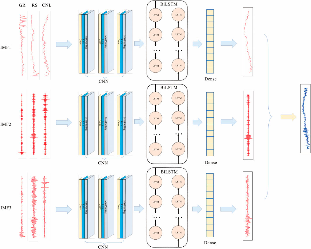
Figure 3. Architecture of VMD-CNN-BiLSTM model.

3.5 Loss function

In this study, a composite loss function combining mean square error (MSE) and soft dynamic time regularization loss (Soft-DTW) (Cuturi and Blondel, 2017; Jiang et al., 2022) is used to balance the optimization objective of local point-by-point error and global morphological similarity in time series forecasting. The traditional MSE loss is sensitive to point-by-point errors, but it is difficult to capture the overall trends and interrelationships of the sequences; Soft-DTW introduces a differentiable approximation to the classical dynamic time warping algorithm through continuous relaxation of alignment paths, thereby enabling direct integration with neural network training frameworks that traditional DTW cannot support due to its non-differentiable nature.

The mean square error (MSE) represents a fundamental loss metric in regression analysis, quantifying the expected squared deviation between predicted and observed values across temporal data points. The formula is shown in Equation 10:

${\mathit{L}}_{\mathit{M}\mathit{S}\mathit{E}}=\frac{1}{\mathit{N}}{\displaystyle \sum _{\mathit{i}=1}^{\mathit{N}}}{\left(\widehat{{\mathit{y}}_{\mathit{i}}}-{\mathit{y}}_{\mathit{i}}\right)}^2(10)$

Where $\widehat{y_i}$ is the predicted value of the ith data point, $y_i$ is the corresponding true value, and N is the total number of data points.

While MSE offers computational advantages including straightforward gradient computation and stable optimization convergence, its underlying assumption of temporal independence limits its ability to capture sequential dependencies and global morphological patterns in time-series data.

Soft Dynamic Time Regularization Loss (Soft-DTW), on the other hand, is an improvement of traditional DTW, aiming at solving its problem of non-trivial discrete path search. The conventional DTW algorithm employs dynamic programming to identify the optimal nonlinear alignment path between temporal sequences, providing an effective measure of global morphological similarity. However, its discrete optimization nature precludes direct integration with neural network architectures for end-to-end learning. Soft-DTW transforms the discrete path selection into continuous probability distributions based on the softmax function through the introduction of the smoothing relaxation technique, making the loss function microscopic. Specifically, a similarity matrix M is constructed between the predicted sequence and the actual sequence, as shown in Equation 11:

${\mathit{M}}_{\mathit{i},\mathit{j}}=\left|\widehat{{\mathit{Y}}_{\mathit{i}}}-{\mathit{Y}}_{\mathit{j}}\right.{|}_2^2(11)$

Where $M_{i,j}$ denotes the squared Euclidean distance for the ith and jth data points.

The accumulation matrix A is then computed by dynamic programming, as shown in Equation 12:

${\mathit{A}}_{\mathit{i},\mathit{j}}={\mathit{M}}_{\mathit{i},\mathit{j}}+\mathit{log}\left(\mathit{exp}\left({\mathit{A}}_{\mathit{i}-1,\mathit{j}}\right)+\mathit{exp}\left({\mathit{A}}_{\mathit{i},\mathit{j}-1}\right)+\mathit{exp}\left({\mathit{A}}_{\mathit{i}-1,\mathit{j}-1}\right)\right)(12)$

Where each element $A_{i,j}$ represents a smooth approximation of the minimum cumulative distance from the starting point (1,1) to (i,j).

The final Soft-DTW loss is the normalized value of the element $A_{T,T}$ in the lower right corner of the accumulation matrix, where T is the length of the sequence. This loss function is insensitive to the time axis offset and can effectively capture the global characteristics of the sequence such as trend and period.

The MSE is finally combined with Soft-DTW to construct the composite loss function, as shown in Equation 13:

${\mathit{L}}_{\mathit{t}\mathit{o}\mathit{t}\mathit{a}\mathit{l}}=\mathit{\lambda }{\mathit{L}}_{\mathit{M}\mathit{S}\mathit{E}}+\left(1-\mathit{\lambda }\right)·{\mathit{L}}_{\mathit{S}\mathit{o}\mathit{f}\mathit{t}-\mathit{D}\mathit{T}\mathit{W}}(13)$

Where $\lambda$ is used to regulate the weights of the two losses as hyperparameters of the model.

4 Experiment and result analysis

4.1 Experimental data

The data of this experiment comes from the open-source logging dataset of Xu et al. (2024), which includes four wells, GY1, C21, SYY1, and YX58, in GL block, and the purpose layer of this experiment is the QSK layer, and the total depth of the four wells is about 1,542 m. The logging curves include the natural gamma (GR), the deep lateral resistivity (RD), the shallow lateral resistivity (RS), the density (DEN), the neutron (CNL), as input features, and acoustic time difference curve (DT) as prediction curve, with a longitudinal sampling rate of 0.125 m.

4.1.1 Data preprocessing

Data standardization process is crucial, the main purpose is to eliminate the influence of the magnitude of different logging curves and to ensure the fair contribution of individual logging curve features to the model results during the model training process. It helps to improve the prediction accuracy and convergence speed of the model. The standardization method used this time is the min-max normalization method, and the normalization formula is shown in Equation 14:

$\mathit{x}=\frac{{\mathit{x}}_{\mathit{i}}-{\mathit{x}}_{\mathit{min}}}{{\mathit{x}}_{\mathit{max}}-{\mathit{x}}_{\mathit{min}}}(14)$

Where $x$ and $x_i$ are the values of the same data point after normalization and before normalization, respectively, and $x_{\mathit{max}}$ and $x_{\mathit{min}}$ are the maximum and minimum values in the features.

After the data processing, the dimensional differences of each well logging curve were eliminated, and the input features had a range of magnitudes of [0,1], while also ensuring the distributional characteristics of the original data (Figures 4, 5).

Figure 4

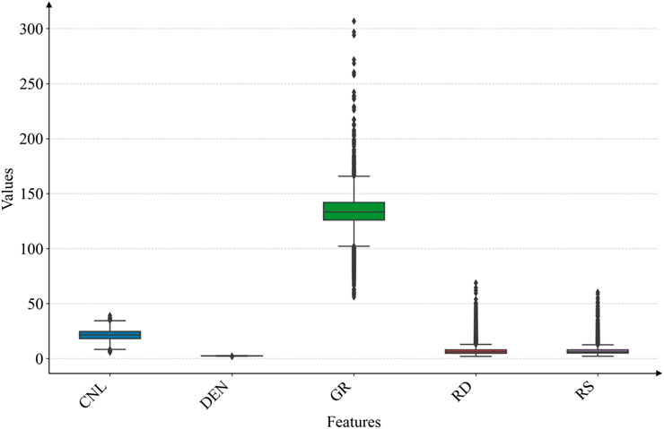
Figure 4. Boxplot of logging data distribution before data normalization.

Figure 5

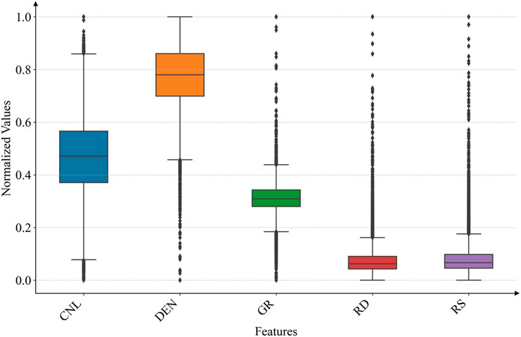
Figure 5. Boxplot of logging data distribution after data normalization.

4.1.2 Feature selection

The accuracy of logging curve reconstruction directly depends on the type of input curve, and optimizing the DT-sensitive curve is the key step. SHAP (SHapleyAdditiveexPlanations), as a powerful feature interpretation tool, can quantify the degree of each feature’s contribution to the model output and the interaction effect between features through the game-theoretic method (Wu et al., 2025). In this logging curve reconstruction analysis, the correlation of different logging curves is first evaluated based on the Person correlation coefficient, and then the influence mechanism of five logging curve features on the target variable DT is analyzed through the XGBoost model combined with the SHAP value, and the sensitive parameters used for DT prediction are screened by combining the two methods.

The magnitude of linear correlation of different logging curves was quantified by Person correlation coefficient analysis, and Figure 6 shows that different logging curves show different positive and negative correlations with DT curves, CNL has the highest correlation coefficient of 0.83 with DT, followed by DEN, which has a negative correlation with a coefficient of 0.58, and the rest of the curves show correlation coefficients of less than 0.5 with DT.

Figure 6

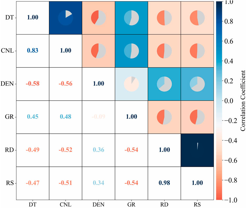
Figure 6. Heat map of pearson correlation coefficient.

The multilinear-nonlinear relationship was further explored by the XGBoost-SHAP method. According to the characteristic importance plot (Figure 7), the mean absolute value of the SHAP value of CNL is the highest (5.43), indicating that it has the most significant influence on the DT prediction, which is consistent with the geologic law to a certain extent, because the neutron curve directly reflects the formation porosity characteristics, and the acoustic time difference is also closely related to the formation porosity. The significance of RS and GR is the next highest, with the significance of 1.52 and 1.30, respectively. DEN and RD have relatively lower importance, 0.99 and 0.82, respectively, probably because they are more complexly affected by lithology and fluid properties, and their direct correlation with DT is weaker.

Figure 7

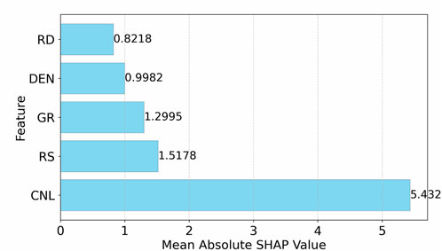
Figure 7. Histogram of importance of features.

The SHAP summary plot (Figure 8) further reveals the direction of the relationship between the eigenvalues and the model output. High values of CNL (red) correspond to positive SHAP values, indicating that high neutron porosity leads to an increase in the DT value. High values of RS and GR also had a positive effect on DT, while DEN showed a negative correlation.

Figure 8

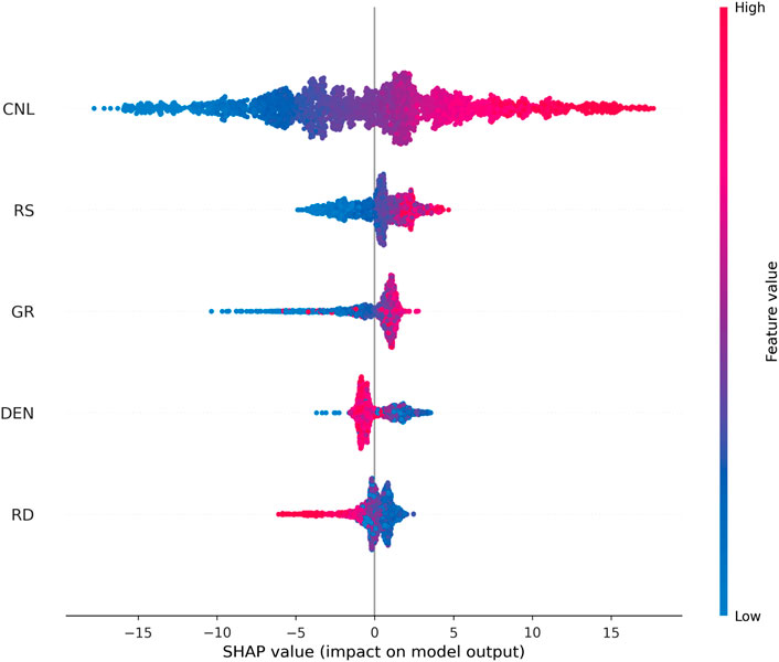
Figure 8. SHAP summary plot (showing the impact and direction of each log feature on DT prediction; color indicates feature magnitude).

The dependence plot and SHAP interaction effect heatmap (Figures 9, 10) indicate that there are significant nonlinear interaction effects among different logging parameters. The synergistic interaction between CNL and RS demonstrates the most pronounced effect (interaction strength = 0.408), indicating their combined influence on DT substantially exceeds the sum of their individual contributions, revealing a non-additive effect. The interaction strength between GR and CNL ranks second at 0.367, while that between RS and RD reaches 0.362. These results suggest a significant interaction enhancement effect between lithology - related curves and porosity - related curves.

Figure 9

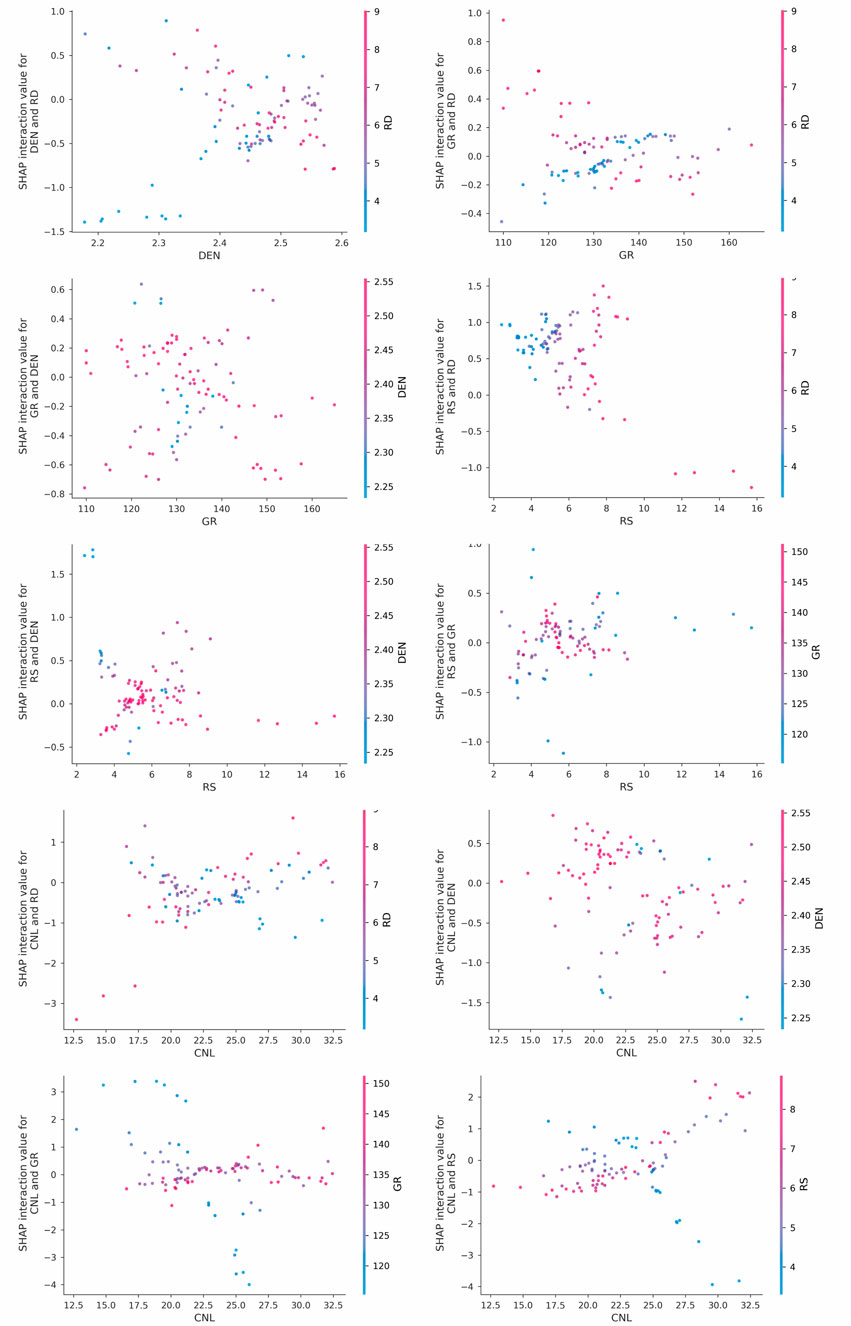
Figure 9. SHAP dependence plot matrix.

Figure 10

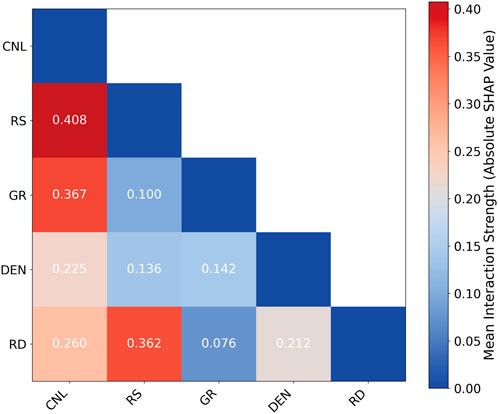
Figure 10. SHAP interaction heatmap.

Based on the importance of a single feature and the feature interaction effect, CNL, RS, and GR are preferred as the key features for predicting DT, although the interaction effect of RD with RS is also stronger, considering that the same resistivity curve will introduce redundant information, the inclusion of RD logging curve is not considered.

4.1.3 Dataset construction

In sequence prediction research, the sliding window method can fully utilize the contextual relevance of long sequence data and is the core method for constructing training samples. The deep sequence data is divided by the sliding window method to construct the sample format that meets the input requirements.

As shown in Figure 11, a fixed window length w and step length s are used for sample set construction, the input features are CNL, RS and GR curves, and the labels are DT curves, and the DT values of the next depth point are predicted with consecutive input curves (CNL, RS, GR) of length w along the direction of increasing depth, and one sample can be constructed within the window for each moving step. A total of 11,986 sample sets were systematically constructed for model development and evaluation. The dataset from wells C21 and GY1 was partitioned into training (80%) and validation (20%) subsets, with the former employed for parameter optimization and the latter for real-time prediction monitoring and overfitting prevention. For independent model assessment, wells SYY1 and YX58 were reserved as hold-out test sets to evaluate practical application performance.

Figure 11

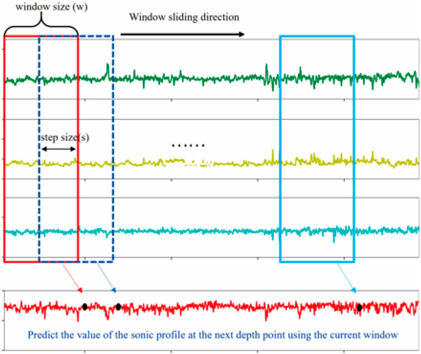
Figure 11. Schematic diagram of the sliding window method.

4.2 Evaluation metrics

This study employs a comprehensive set of quantitative metrics to assess the model’s performance in curve reconstruction tasks. Four key evaluation indicators are utilized: Mean Squared Error (MSE), Mean Absolute Error (MAE), Coefficient of Determination (R²), and Mean Absolute Percentage Error (MAPE). Among these metrics, MSE and MAE primarily measure the magnitude of absolute deviations between the reconstructed curves and their corresponding ground truth values. The former emphasizes the overall degree of dispersion, while the latter highlights the magnitude of the average deviation. To evaluate the model’s curve-fitting capability from the perspective of variance interpretation, the R² quantifies how well the reconstructed curves explain the variance in the original data. MAPE is a relative error measure that eliminates the impact of dimensions. The formula for MSE is shown in Equation 10 and the calculations for the other indicators are shown in Equations 15–17:

$\text{MAE}=\frac{1}{\mathit{m}}{\displaystyle \sum _{\mathit{i}=1}^{\mathit{m}}}\left|\widehat{{\mathit{y}}_{\mathit{i}}}-{\mathit{y}}_{\mathit{i}}\right|(15)$

${\mathit{R}}^2=1-\frac{{\displaystyle {\sum }_{\mathit{i}=1}^{\mathit{m}}}{\left(\widehat{{\mathit{y}}_{\mathit{i}}}-{\mathit{y}}_{\mathit{i}}\right)}^2}{{\displaystyle {\sum }_{\mathit{i}=1}^{\mathit{m}}}{\left(\overline{\mathit{y}}-{\mathit{y}}_{\mathit{i}}\right)}^2}(16)$

$\text{MAPE}=\frac{1}{\mathit{m}}{\displaystyle \sum _{\mathit{i}=1}^{\mathit{m}}}\left|\frac{{\mathit{y}}_{\mathit{i}}-\widehat{{\mathit{y}}_{\mathit{i}}}}{{\mathit{y}}_{\mathit{i}}}\right|\times 100\%(17)$

Where $m$ is the number of samples, $y_i$ denotes the true value of the ith sample, and $\widehat{y_i}$ is the corresponding model prediction.

Lower values of MSE, MAE, and MAPE indicate higher reconstruction accuracy, while an R² value closer to 1 reflects better curve-fitting performance.

4.3 Experimental process

The workflow for reconstructing the DT curve based on the model proposed in this paper is shown in the Figure 12. First, preprocessing is performed on the collected curves, including outlier removal and normalization. Then, the optimized CNL, RS, and GR curves are decomposed using VMD. Additionally, the DT curve to be predicted also undergoes decomposition. On this basis, prediction models are established for each component IMF. Finally, all predicted values are superimposed to obtain the final reconstructed curve.

Figure 12

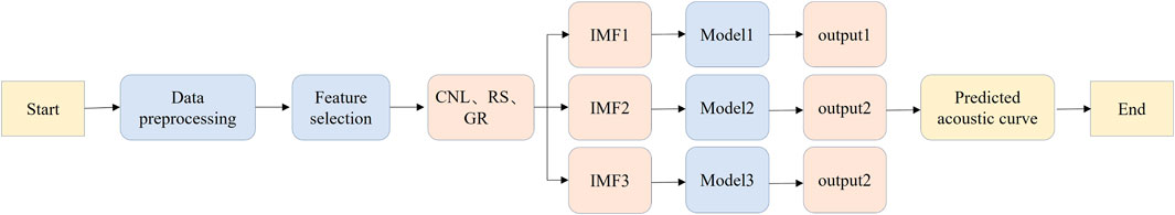
Figure 12. Algorithmic process.

4.4 Model training

The experiment was run on Window11 operating system, using Python programming language and Tensorflow deep learning framework, using a computer configuration of NVIDIA RTX 3090 with 16G video memory. The model uses the above combination function as the loss function and the Adam optimizer, and the individual hyperparameters of the experiment are set as follows, with the Batchsize set to 32, the initial learning rate set to 0.01, $\lambda$ set to 0.7, and 64 training iterations.

Figure 13 shows the trend of the loss values of different component prediction models after VMD decomposition with the number of iterations, and it can be seen that with the increase of the number of training times, the loss values of the model are decreasing, and gradually converge to a stable state, and finally reach the convergence state.

Figure 13

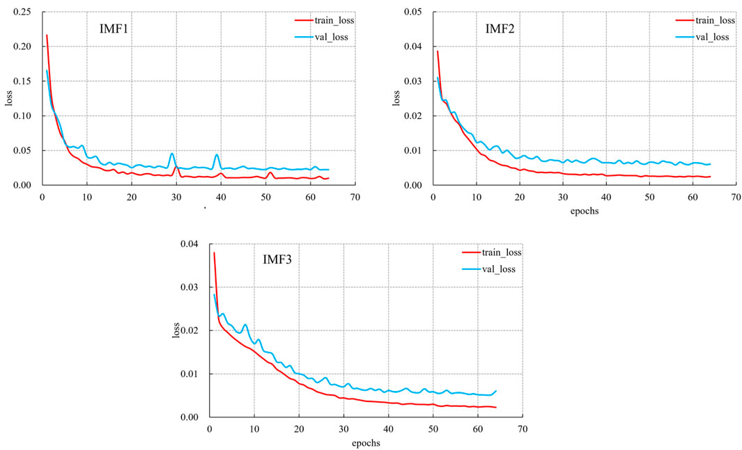
Figure 13. Loss function descent plot.

4.5 Application effect analysis

The trained model is applied to two test wells, thus demonstrating the practical application effect of the model.

Figures 14, 15 respectively present the scatter plots comparing the predicted and measured values of the acoustic time difference (DT) for the SYY-1 well and the YX58 well. The scattered points are mainly distributed near the 45° diagonal line, indicating a good linear consistency between the two. Specifically, for Figure 14 (SYY-1 well), the coefficient of determination R² is 0.8783, and the slope of the regression equation is 0.8231; for Figure 15 (YX58 well), the coefficient of determination R² is 0.7142, and the slope of the regression equation is 0.6354. There is a certain difference in the prediction results of the two wells. This is because the similarity of the logging curves between the YX58 well and the training well is lower than that of the SYY1 well, and at the same time, the formation thickness of the YX58 well is much smaller than that of the training well (Wu et al., 2024), reflecting the differences in sedimentary characteristics. Therefore, the difference in the prediction results of the two wells is acceptable. Furthermore, single-well logging curves are plotted. In the DT curve track of Figure 16, the blue and yellow curves denote the true and predicted values, respectively. The results demonstrate that the proposed method achieves accurate predictions for the acoustic curves in both wells. Specifically, the predicted curve closely follows the overall trend of the true curve, effectively capturing its amplitude variations. Furthermore, the model reliably reproduces key features, including peak and valley positions, indicating strong agreement between predictions and ground truth. This indicates that the model can effectively uncover the correlations among different logging curves, and learn the local undulation characteristics, long-distance variation trends, and sequential correlations of the curves.

Figure 14

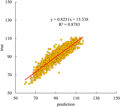
Figure 14. Scatterplot of raw and predicted acoustic curve values for SYY1 well.

Figure 15

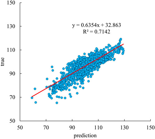
Figure 15. Scatterplot of raw and predicted acoustic curve values for YX58 well.

Figure 16

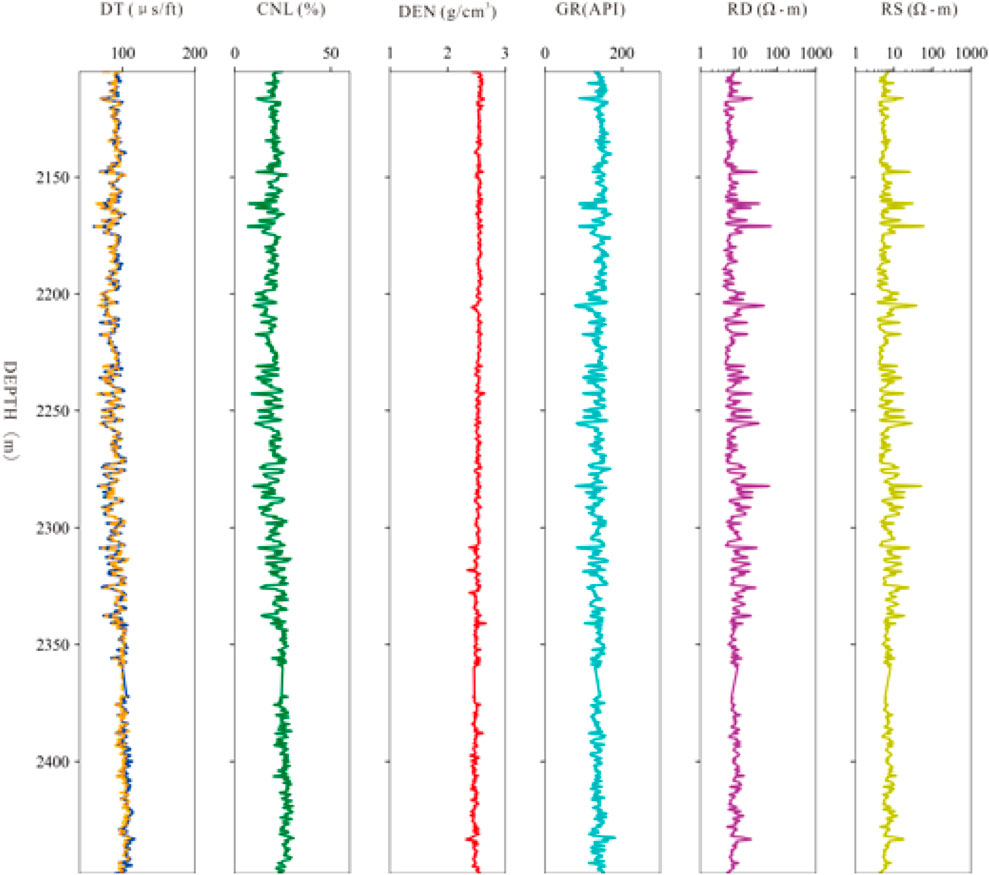
Figure 16. Logging curve of SYY1 well (Tracks from left to right: DT (yellow = VMD-CNN-BiLSTM prediction, blue = measured), CNL, DEN, GR, RD, and RS).

4.6 Comparison experiments

To validate the effectiveness of the proposed method, we conducted comparative experiments against several conventional machine learning approaches, including Support Vector Regression (SVR), Random Forest, and standard LSTM models. The performance metrics of these models on the validation set are presented in Table 1, enabling a comprehensive evaluation of their relative strengths and limitations.

Table 1

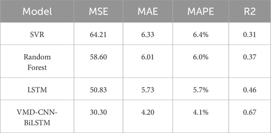
Table 1. Evaluation metrics performance of different models on the test set.

From the data in the table, it can be seen that the VMD-CNN-BiLSTM model shows the optimal performance with MSE of 30.30, MAE of 4.20, MAPE of 0.041, and the fitting effect of R² reaches 0.67. Compared with the other models, it has reduced the error metrics, significantly improved the prediction accuracy, and the best reconstruction of acoustic wave curves.

The performance of the models can be further visualized from the corresponding test well prediction curve plots (Figure 17), where the green curve represents the predicted value and the blue curve represents the true labeled value. The SVR model exhibits significant deviations from the true curves in both morphological structure and absolute values, particularly in high-variability segments where prediction errors are most pronounced. While the Random Forest model demonstrates measurable improvement over SVR, it still shows limitations in capturing fine-scale variations. The LSTM model achieves superior performance overall, faithfully reconstructing the general trend of true curves across most depth intervals. However, its predictive accuracy diminishes in zones of rapid curve fluctuation, notably around the 2000 m depth region where complex patterns emerge. The VMD-CNN-BiLSTM model is the closest to the real labeled curves, and it can reconstruct the overall trend of the curves and the local peaks and valleys in the whole depth range. The results show that the VMD-CNN-BiLSTM model has better application in logging curve reconstruction.

Figure 17

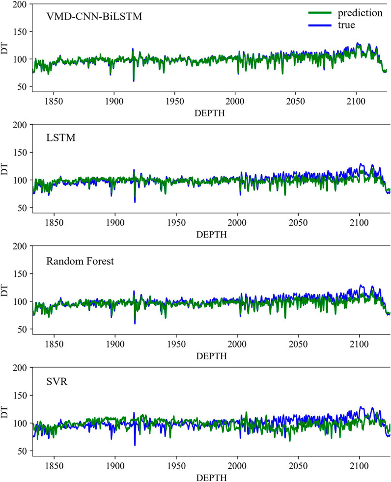
Figure 17. Comparison of different model prediction results and real logging curve of well YX58.

5 Conclusion

Aiming at the problems of missing and distorted data caused by irresistible factors during the acquisition of logging curves, this paper applies a VMD-CNN-BiLSTM cascade network model for DT reconstruction considering logging curves as a kind of depth sequence data, which has a good application in sequence prediction tasks. Through comprehensive feature selection, we identified CNL, GR, and RS curves as optimal input features due to their strong correlation with target variables. The variational mode decomposition (VMD) method was employed to decompose these curves into intrinsic mode functions. Distinct prediction models were then developed for each frequency component, with the final reconstruction achieved through superposition of all modal predictions.

This method breaks through the limitations of traditional feature selection based on linear correlation and point-to-point prediction in machine learning. It introduces the XGBoost-SHAP method to screen important features in a way that is interpretable, and innovatively implements a time series modeling model based on feature decomposition. Compared with traditional machine learning and simple long short-term memory neural networks, this method achieves better reconstruction results. Additionally, this method can be extended to reconstruct other well logging curves by adjusting parameters, and can also be used to train and predict well logging curve for other strata by adjusting the data set. This research to some extent can provide certain reference significance for tasks such as well logging curve reconstruction or completion.

Data availability statement

The original contributions presented in the study are included in the article/supplementary material, further inquiries can be directed to the corresponding author.

Author contributions

HW: Data curation, Conceptualization, Investigation, Writing – original draft, Methodology, Writing – review and editing, Formal Analysis. YZ: Data curation, Writing – review and editing, Conceptualization, Formal Analysis. JL: Software, Investigation, Validation, Writing – review and editing, Conceptualization. ST: Validation, Writing – review and editing, Investigation, Software. YW: Software, Investigation, Validation, Writing – review and editing. XS: Validation, Investigation, Software, Writing – review and editing. MZ: Validation, Writing – review and editing, Investigation, Software. SL: Software, Writing – review and editing, Investigation, Validation. ZL: Validation, Investigation, Writing – review and editing, Software.

Funding

The author(s) declare that no financial support was received for the research and/or publication of this article.

Conflict of interest

Authors HW, YZ, JL, ST, YW, XS, MZ, SL, and ZL were employed by Shandong Leading Petro-Tech Co., Ltd.

Generative AI statement

The author(s) declare that no Generative AI was used in the creation of this manuscript.

Any alternative text (alt text) provided alongside figures in this article has been generated by Frontiers with the support of artificial intelligence and reasonable efforts have been made to ensure accuracy, including review by the authors wherever possible. If you identify any issues, please contact us.

Publisher’s note

All claims expressed in this article are solely those of the authors and do not necessarily represent those of their affiliated organizations, or those of the publisher, the editors and the reviewers. Any product that may be evaluated in this article, or claim that may be made by its manufacturer, is not guaranteed or endorsed by the publisher.

References

Afifi, R., and Anifowose, F. (2023). “Compressional sonic log prediction experiment using machine learning: Algorithms and feature selection,” in Paper presented at the Fifth EAGE Borehole Geology Workshop, Riyadh, Saudi Arabia (EAGE). doi:10.3997/2214-4609.2023631004

CrossRef Full Text | Google Scholar

Aftab, S., Moghadam, R. H., and Leisi, A. (2023). New interpretation approach of well logging data for evaluation of kern aquifer in south California. J. Appl. Geophys. 215, 105138. doi:10.1016/j.jappgeo.2023.105138

CrossRef Full Text | Google Scholar

Chen, G. H., and Wang, Y. G. (2005). Application of Faust formula in acoustic curve reconstruction. Prog. Exploration Geophys. (02), 125–128+10.

Google Scholar

Cuturi, M., and Blondel, M. (2017). “Soft-dtw: a differentiable loss function for time-series,” in International Conference on Machine Learning (PMLR), 894–903.

Google Scholar

Dragomiretskiy, K., and Zosso, D. (2013). Variational mode decomposition. IEEE Trans. Signal Process. 62 (3), 531–544. doi:10.1109/tsp.2013.2288675

CrossRef Full Text | Google Scholar

Gama, P. H. T., Faria, J., Sena, J., Neves, F., Riffel, V. R., Perez, L., et al. (2025). Imputation in well log data: a benchmark for machine learning methods. Comput. Geosciences 196, 105789. doi:10.1016/j.cageo.2024.105789

CrossRef Full Text | Google Scholar

Hochreiter, S., and Schmidhuber, J. (1997). Long short-term memory. Neural Comput. 9 (8), 1735–1780. doi:10.1162/neco.1997.9.8.1735

PubMed Abstract | CrossRef Full Text | Google Scholar

Ibrahim, A. F., and Elkatatny, S. (2022). Real-time GR logs estimation while drilling using surface drilling data; AI application. Arabian J. Sci. Eng. 47 (9), 11187–11196. doi:10.1007/s13369-021-05854-7

CrossRef Full Text | Google Scholar

Jiang, J. J., Lai, S. X., Jin, L. W., and Zhu, Y. (2022). Dsdtw: local representation learning with deep soft-dtw for dynamic signature verification. IEEE Trans. Inf. Forensics Secur. 17, 2198–2212. doi:10.1109/tifs.2022.3180219

CrossRef Full Text | Google Scholar

Kim, M. J., and Cho, Y. (2024). Imputation of missing values in well log data using k-nearest neighbor collaborative filtering. Comput. Geosciences 193, 105712. doi:10.1016/j.cageo.2024.105712

CrossRef Full Text | Google Scholar

Li, Z. H., and Jiang, S. (2025). Based on machine learning and SHAP algorithm of acoustic well logging curve recon-struction and interpretability analysis. Bull. Geotechnical Sci. Eng. 44 (01), 321–331. doi:10.19509/j.cnki.dzkq.tb20230504

CrossRef Full Text | Google Scholar

Li, N., Yu, P., Tian, J., and Xu, B. X. (2016). Discussion on acoustic and density well logging curve reconstruction method for reservoir prediction of Longfengshan Yingcheng formation—A case study of well LB1. Oil and Gas Reserv. Eval. Dev. 6 (04), 18–22. doi:10.13809/j.cnki.cn32-1825/te.2016.04.004

CrossRef Full Text | Google Scholar

Li, F. L., Liu, H. S., Yang, X. L., Zhao, M. X., Yang, C., and Zhang, L. C. (2023). Based on U-Net neural network of acoustic well logging curve reconstruction. J. Ocean Univ. China 53 (08), 86–92+103. doi:10.16441/j.cnki.hdxb.20220239

CrossRef Full Text | Google Scholar

Liao, M. H. (2014). Correction of the influence of expansion on density and acoustic curves using multiple re-gression methods. Geophys. Prospect. 38 (01), 174–179+184.

Google Scholar

Liu, D., Wang, Q., You, N., Sacchi, M. D., and Chen, W. (2024). Filling the gap: enhancing borehole imaging with tensor neural network. *Geophysics*, 1–64. doi:10.1190/geo2024-0242.1

CrossRef Full Text | Google Scholar

Liu, J. J., Zhou, J., Yu, W. D., Chen, J. H., Fan, Q., and Yan, G. H. (2024). Based on hyperparameter optimized LSTM of acoustic well logging curve generation technology. Petroleum Geophysics 63 (05), 1061–1074.

Google Scholar

Nero, C., Aning, A. A., Danuor, S. K., and Mensah, V. (2023). Prediction of compressional sonic log in the western (Tano) sedimentary basin of Ghana, West Africa using supervised machine learning algorithms. Heliyon 9 (9), e20242. doi:10.1016/j.heliyon.2023.e20242

PubMed Abstract | CrossRef Full Text | Google Scholar

Qu, F. T., Xu, Y. Q., Liao, H. L., Liu, J., Geng, Y., and Han, L. (2025). Missing data interpolation in well logs based on genera-tive adversarial network and improved krill herd algorithm. Geoenergy Science and Engineering 246, 213538. doi:10.1016/j.geoen.2024.213538

CrossRef Full Text | Google Scholar

Redwan, U. G., Zaman, T., and Mizan, H. B. (2025). Spatio-temporal CNN-BiLSTM dynamic approach to emotion recog-nition based on EEG signal. Computers in Biology and Medicine 192 (Pt A), 110277. doi:10.1016/j.compbiomed.2025.110277

PubMed Abstract | CrossRef Full Text | Google Scholar

Saleh, K., Mabrouk, W. M., and Metwally, A. (2025). Machine learning model optimization for compressional sonic log prediction using well logs in Shahd SE field, Western Desert, Egypt. Scientific Reports 15, 14957. doi:10.1038/s41598-025-97938-9

PubMed Abstract | CrossRef Full Text | Google Scholar

Shang, F. H., Lu, Y. Y., and Cao, M. J. (2022). Based on improved LSTM neural network of well logging curve reconstruc-tion method. Computer Technology and Development 32 (06), 198–202.

Google Scholar

Wang, J. R., Liang, L. W., Deng, Q., Tian, P. P., and Tan, W. X. (2016). Research and application of well logging curve recon-struction method based on multiple regression model. Lithologic Reservoirs 28 (03), 113–120.

Google Scholar

Wang, J., Cao, J. X., and You, J. C. (2020). Based on GRU neural network of well logging curve reconstruction. Petroleum Earth Physics Exploration 55 (03), 510–520+468. doi:10.13810/j.cnki.issn.1000-7210.2020.03.004

CrossRef Full Text | Google Scholar

Wu, T. F., Wang, M., Xi, Y. F., and Zhao, Z. C. (2024). Intent recognition model based on sequential information and sen-tence features. Neurocomputing, 566. doi:10.1016/j.neucom.2023.127054

CrossRef Full Text | Google Scholar

Wu, Z. Z., Wang, S. Z., Li, L. Y., and Suo, Y. (2025). An interpretable ship risk model based on machine learning and SHAP interpretation technique. Ocean Engineering 335, 121686. doi:10.1016/j.oceaneng.2025.121686

CrossRef Full Text | Google Scholar

Xu, B. S., Zhou, F., Zhou, J., Shao, R., Wu, H., Liu, P., et al. (2024). Transfer learning for well logging formation evaluation using similarity weights. Artificial Intelligence in Geosciences 5, 100091. doi:10.1016/j.aiig.2024.100091

CrossRef Full Text | Google Scholar

Yin, J. Y., Wang, X. J., Yang, R. R., Xie, Z. R., and Liu, Z. Q. (2014). Application of multi-well logging curve pseudo-acoustic re-construction technology. Xinjiang Petroleum Geology 35 (04), 461–465.

Google Scholar

Yuan, Q. S., Zhou, J. X., Li, Y., and Zhang, G. D. (2009). The application of acoustic well logging curve reconstruction tech-nology in reservoir prediction. China Offshore Oil and Gas 21 (01), 23–26.

Google Scholar

Zhai, X. Y., Gao, G., Li, Y. G., Chen, D., Gui, Z. X., and Wang, Z. Z. (2023). Fusion attention mechanism of two-dimensional con-volutional neural network well logging curve reconstruction method. Petroleum Earth Physics Exploration 58 (05), 1031–1041. doi:10.13810/j.cnki.issn.1000-7210.2023.05.001

CrossRef Full Text | Google Scholar

Zhan, W., Chen, Y., Liu, Q., Li, J., Sacchi, M. D., Zhuang, M., et al. (2024). Simultaneous prediction of petrophysical properties and formation layered thickness from acoustic logging data using a modular cascading residual neural network (MCARNN) with physical constraints. *Journal of Applied Geophysics* 224, 105362. doi:10.1016/j.jappgeo.2024.105362

CrossRef Full Text | Google Scholar

Zhang, J. C., Deng, J. G., Tan, Q., and Shi, L. (2022). Well logging curve reconstruction method based on XGBoost. Petroleum Earth Physics Exploration 57 (03), 697–705+496. doi:10.13810/j.cnki.issn.1000-7210.2022.03.020

CrossRef Full Text | Google Scholar

Zhang, H. Y., Wu, W. S., Chen, Z. X., and Jing, J. (2024). Well logs reconstruction of petroleum energy exploration based on bidirectional long Short-term memory networks with a PSO optimization algorithm. Geoenergy Science and Engineering 239, 212975. doi:10.1016/j.geoen.2024.212975

CrossRef Full Text | Google Scholar

Zhao, P. Q., Zhuang, W., Sun, Z. C., Wang, Z., Luo, X., Mao, Z., et al. (2016). Methods for estimating petrophysical parameters from well logs in tight oil reservoirs: a case study. Journal of Geophysics and Engineering 13 (01), 78–85. doi:10.1088/1742-2132/13/1/78

CrossRef Full Text | Google Scholar

Zhou, W., Zhao, H. H., Jiang, Y. F., Yi, J., and Lai, F. Q. (2022). Based on the cascaded bidirectional long short-term memory neural network of well logging data reconstruction. Petroleum Earth Physics Exploration 57 (06), 1473–1480+1263. doi:10.13810/j.cnki.issn.1000-7210.2022.06.023

CrossRef Full Text | Google Scholar

Zhou, W., Zhao, H. H., Li, X. C. Z., Qi, Z., Lai, F., and Yi, J. (2025). Missing well logs reconstruction based on cascaded bidi-rectional long short-term memory network. Expert Systems with Applications 259, 125270. doi:10.1016/j.eswa.2024.125270

CrossRef Full Text | Google Scholar