Susceptibility assessment of freeze-thaw erosion induced debris flow using random forest, Eastern Tibetan Plateau

Machine learning algorithms have shown excellent results in susceptibility assessment of debris flow hazards in different areas. These results depend on selecting control factors that align with the actual conditions of the study area. Due to the hazard’s formation conditions, alpine experience significantly advanced freeze-thaw erosion, yet current research seldom considers this as a controlling factor. Consequently, this study selects the northern area of the Gongjue Basin in the Eastern Tibetan Plateau, where the freeze-thaw erosion plays a controlled driving force for debris flow. The primary emphasis is on investigating the influence of freeze-thaw erosion on the debris flow susceptibility assessment model. To this end, a statistical analysis was performed on the frequency and overall performance of control factors chosen in relevant literature on debris flow susceptibility assessment using machine learning. Control factors with high frequency and performance were selected from the perspectives of material sources, dynamic conditions, and hydrological factors, leading to an optimized selection strategy, and the Random Forest Algorithm was employed for susceptibility assessment (No Freeze-thaw erosion model, NFEM). Subsequently, the freeze-thaw erosion index, a new control factor gauging the intensity of freeze-thaw erosion in the study area, was incorporated, and the susceptibility assessment was also conducted using the Random Forest Algorithm (Freeze-thaw erosion model, FEM). The results show that FEM improved accuracy by 0.457 and AUC by 0.0541 compared to NFEM, indicating enhanced predictive performance. Nevertheless, when comparing watershed samples, both models demonstrated limited predictive power. In terms of susceptibility outcomes, FEM yielded more precise assessment results based on the available data.

1 Introduction

Debris flow, a common sudden geological hazard in mountainous areas, is characterized by rapid onset and strong destructiveness. It often causes traffic disruption, damage to infrastructure, and even casualties, posing a serious threat to ecological security and human activities in high-altitude mountainous regions (Guzzetti et al., 1999; Kumar and Sarkar, 2023). In high-altitude cold regions such as the eastern Tibetan Plateau, freeze-thaw erosion, as a special surficial geological process, damages the structure of rock and soil through repeated freeze-thaw cycles, generating a large amount of loose debris and providing a key material source for debris flows (Huang et al., 2021). However, in current studies on debris flow susceptibility in this region, the role of freeze-thaw erosion as a contributor to material sources is often overlooked, making it difficult for the assessment results to accurately reflect the particularities of hazards in cold regions. Therefore, how to incorporate the effect of freeze-thaw erosion into the evaluation of debris flow susceptibility has become a key scientific issue for improving the accuracy of geological hazard assessment in cold regions.

Debris flow susceptibility assessment refers to the spatial quantitative evaluation of the possibility and difficulty of debris flow occurrence in different regions within a specific geographical environment. Its core is to reveal the relationship between “hazard-pregnant environmental conditions” and “probability of debris flow occurrence”, and does not directly involve dynamic characteristics such as the time and scale of disaster occurrence (Kumar and Sarkar, 2023). As a basic link in disaster risk assessment, susceptibility assessment can provide a scientific basis for territorial spatial planning and the layout of disaster prevention and mitigation projects, and has important practical significance for reducing disaster losses (Guzzetti et al., 1999). In recent years, with the development of 3S technology and artificial intelligence, debris flow susceptibility assessment methods have evolved from traditional models to intelligent ones. Early empirical models (such as analytic hierarchy process, fuzzy logic) and statistical models (such as frequency ratio, information value method) rely on manual assignment or linear assumptions, making it difficult to capture nonlinear relationships in complex hazard-pregnant environments (Achour et al., 2018; Chen et al., 2015; Wang et al., 2014; Xu et al., 2013; Zhang et al., 2022). In contrast, machine learning models (such as logistic regression, support vector machine, random forest) mine factor correlations through data-driven methods, showing significant advantages in assessment accuracy and have become the mainstream method in current research (Behnia and Blais-Stevens, 2018; Huang et al., 2022; Wu et al., 2019; Xiong et al., 2020). Existing studies mainly focus on two aspects: first, selecting the optimal method suitable for specific regions through multi-model comparison (Di et al., 2019; Gu et al., 2023; Liang et al., 2020; Qing et al., 2020); second, improving assessment performance by optimizing sample quality, improving feature factors, or constructing hybrid models (Cao et al., 2023; Dong and Wu, 2022; Gao et al., 2021; Li et al., 2023; Liang et al., 2023; Qin et al., 2022; Zhang et al., 2019).

Although machine learning models are widely used, the scientific selection of control factors remains a key bottleneck restricting assessment accuracy. Most existing studies select factors from conventional dimensions such as topography, geology, hydrology, and vegetation (Reichenbach et al., 2018; Kumar and Sarkar, 2023), but generally ignore the impact of region-specific processes. In high-altitude cold regions, freeze-thaw erosion directly controls the formation and distribution of debris flows by changing the mechanical properties of rock and soil and providing loose materials (Huang et al., 2021). However, its role is often simplified as an indirect representation of topographic (such as slope, elevation) or geological (such as lithology) factors, and has not been included in the assessment model as an independent control factor. This simplification makes it difficult for the model to distinguish the essential differences between freeze-thaw erosion induced debris flows and other types of debris flows, potentially overestimating or underestimating disaster risks in key cold-region areas.

To address the above issues, this study takes the northern part of the Gongjue Basin in the eastern Tibetan Plateau as the study area (where freeze-thaw erosion is strong and serves as the main supply mechanism of debris flow materials), focusing on exploring the impact of freeze-thaw erosion on debris flow susceptibility assessment. The research ideas include: (1) Through statistical analysis of literature, screen out high-frequency and high-efficiency control factors in machine learning assessment, and construct a basic factor system covering material source, dynamic, and hydrological conditions; (2) Introduce the freeze-thaw erosion index (FEI) as a new factor to quantify freeze-thaw intensity, and construct the “Freeze-thaw Erosion Model (FEM)” and “No Freeze-thaw Erosion Model (NFEM)” respectively based on the random forest algorithm; (3) By comparing the assessment accuracy and susceptibility zoning results of the two models, reveal the mechanism and necessity of the freeze-thaw erosion factor. This study aims to provide more accurate methodological support for debris flow susceptibility assessment in cold regions and offer guidance for regional disaster prevention and mitigation engineering construction.

2 Study area and materials

2.1 Study area

The study area is situated in the southeastern part of the Gongjue Basin, within Gongjue County and Chaya County, Qamdo City, at geographic coordinates E98°14′to E98°30′and N30°30′to N31°00′. The altitude varies between 3470 m and 5012 m, and the terrain undergoes significant changes. The overall terrain is characterized by high mountains on the northeast and southwest sides, and a low-lying basin in the central part cut by multiple rivers. The primary rivers are the Wa River and Ma River, with Ma River flowing from north to south through the center of the study area (Figure 1). The exposed strata primarily consist of Triassic to Jurassic layers and Paleogene strata, predominantly composed of sandstone, limestone, and mudstone. Intense tectonic activity has resulted in the significant development of faults and folds in the region. The main faults include the Kadolado, Chuandehe, Kuoda, Ladoniuchang, Rijian, and Wenza faults, while the principal folds are the Ruige and Rannongka synclines.

Figure 1

Figure 1. Geographical location and distribution of debris flow points in the study area. (a) Location of Qamdo. (b) Location of study area. (c) Study area.

The study area experiences a continental plateau monsoon climate, influenced by latitude, elevation, and geographic location. Temperatures are generally low, with significant diurnal temperature variations, and soil temperatures are lower than air temperatures, leading to prolonged periods of permafrost. Consequently, the moisture content in the soil and rock fluctuates with temperature changes. During the day, prolonged sunlight and intense radiation cause higher temperatures, leading to the melting of moisture within the soil and rock into liquid form. At night, temperatures drop, and the soil temperature falls below the freezing point of water, causing liquid water to freeze into solid ice. Repeated freeze-thaw cycles cause changes in the volume of water within the soil and rock, altering their microstructure and mechanical properties, ultimately leading to deformation and failure (Figures 2a,b). Field investigations reveal the frequent presence of freeze-thaw eroded bedrock in various states within the gullies of the study area. This erosion process supplies abundant material for debris flow formation.

Figure 2

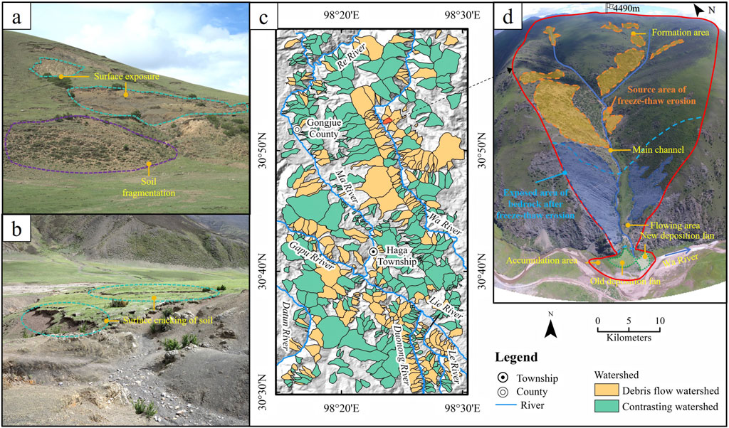
Figure 2. Survey situation of the study area. (a) The freeze-thaw erosion process leads to surface exposure. (b) The freeze-thaw erosion process causes cracks in the topsoil. (c) Distribution of positive and negative samples in the study area. (d) Overview of a typical debris flow watershed.

2.2 Debris flow inventory

A comprehensive and accurate inventory of debris flows is fundamental for assessing susceptibility. This study establishes a debris flow inventory by combining remote sensing interpretation and engineering geological surveys with a precision of 1:50,000.The acquisition of images and on-site investigations were completed by August 2023. Initially, preliminary remote sensing interpretation was employed to identify watersheds within the study area that exhibited clear signs of debris flow activity. Those meeting the following criteria will be initially judged as positive samples: they present typical debris flow landforms in at least one phase of satellite images, with fan-shaped deposits at the gully mouths and clear fan boundaries (showing “fan-shaped radial textures” in the images), and belt-like or strip-like erosion traces or fresh deposits formed by recent activities (with significantly different tones from the surrounding areas) can be seen in the main gullies. This step involved collecting multi-source, multi-temporal high-resolution satellite images (The remote sensing images in this study are derived from https://mapcube.21atcloud.com.cn/, from 2000 to August 2023). Currently, debris flow remote sensing interpretation is mainly categorized into two methods: automatic recognition based on high-resolution images and traditional manual visual interpretation. Automatic recognition, which uses computer vision technology to identify debris flows through modeling, is more efficient but less accurate (Bregoli et al., 2015). Manual visual interpretation, conducted by experts relying on their experience and knowledge, is less efficient but generally more accurate (Pourghasemi and Rahmati, 2018). Therefore, we opted for manual visual interpretation to ensure the accuracy of the results. Subsequently, we verified and supplemented the preliminary interpretation results through field investigations, removing watersheds with unclear or uncertain signs of activity, and supplementing debris flow watersheds that were not identified by remote sensing interpretation. A watershed was finally confirmed as a positive sample if obvious signs of debris flow activity were found in it (such as debris flow deposits, fan-shaped boundaries formed by the flow rushing out of the gully mouth, scratches or steep slopes on both sides of the valley mountains, etc.) or if there were disaster events recorded by local residents. The positive samples supplemented and confirmed through field investigations include not only the debris flows that occurred in the past 20 years, which were initially identified by remote sensing interpretation, but also older debris flows. They also include watersheds where obvious signs of debris flow activity can be observed but the occurrence time is unknown. Based on satellite image analysis and field investigations, we identified 362 debris flows larger than 0.03 km² within a rectangular area of approximately 1,540 km², covering a total area of 458 km². Due to the geological and meteorological conditions in the study area, freeze-thaw erosion is evident in these debris flow watersheds, providing abundant material sources for debris flow outbreaks. Hence, they are referred to as freeze-thaw erosion induced debris flows. The resulting debris flow density was calculated as 0.235 per km² (362/1,540 km²), with a debris flow area percentage of 29.74% (458 km²/1,540 km² × 100%).

Selecting appropriate mapping units is crucial for ensuring the accuracy and usability of the DFS assessment. Common mapping units include grid units and watershed units. Grid units are easy to calculate but do not reflect geological conditions or have a physical relationship with debris flows (Nefeslioglu et al., 2008; Zhu et al., 2019). Watershed units can fully represent the terrain and geological conditions relevant to debris flow development and activity (Liu et al., 2024; Reichenbach et al., 2018). In this study, watershed units were used as the mapping units, and the watershed boundaries were delineated using the same methods of remote sensing interpretation and field investigations employed in establishing the debris flow inventory. Firstly, high-resolution remote sensing images were used to identify topographic features and debris flow accumulation characteristics, and preliminary watershed boundaries were manually delineated using DEM data. Subsequently, for areas with uncertain interpretation results such as topographically complex regions and vegetation-covered areas, field GPS surveys and verification using UAV aerial surveys were conducted to revise the boundaries.This method, which integrates the texture features of remote sensing images with manual delineation, can avoid the problems of boundary deviation that ArcGIS is prone to caused by data errors. Meanwhile, by identifying historical debris flow traces through field investigations, this method ensures that the watershed units can completely cover the entire process of disasters from outbreak to accumulation. In contrast, the automatic extraction by ArcGIS may lead to watershed fragmentation due to improper settings of confluence thresholds. Therefore, this method is more reliable and accurate than the commonly used method of automatically extracting watersheds with ArcGIS hydrological analysis tools, and can ensure the continuity of debris flow events within the watershed units.

To maintain model balance, we generated a certain number of negative samples in the study. Common methods for generating negative samples include random sampling (Melton, 1966; Pourghasemi and Rahmati, 2018) and buffer-controlled sampling (Schumm, 1956), but neither guarantees sample accuracy. To overcome this limitation, we also interpreted watersheds where no debris flow events had occurred during the interpretation process, conducting field surveys to verify the accuracy. The selection of negative samples meets the following criteria: in all available remote sensing images from 2000 to 2022, there are no signs of activities such as debris flow deposits or gully erosion, and there are no abrupt changes in vegetation coverage or topographic morphology within the watershed (e.g., no newly added exposed areas); field investigations confirm that there are no loose deposits accumulated in the watershed, no records of historical disasters, and the current terrain (such as gentle gullies, exposed dense bedrock) does not meet the basic conditions for debris flow formation. Due to limitations in satellite imagery and transportation conditions, we ultimately identified 220 watersheds where no debris flow events had occurred, which served as negative samples (Figure 2c). This method provided us with a set of negative samples that are more representative than those obtained through random or buffer-controlled sampling. In the end, we obtained 582 samples, including 362 positive samples and 220 negative samples, resulting in a ratio of 1.65:1.

3 Methodology

3.1 Selection and analysis of debris flow controlling factors

3.1.1 Analysis of debris flow control factors in machine learning

The occurrence of debris flows is a highly complex process influenced by numerous factors. Currently, there is no standardized guideline for selecting factors that control debris flow susceptibility. Most existing studies choose these factors based on data availability, integrating considerations from topography, geology, hydrology, and land cover, while also considering the specific geological conditions of the study area. Through the Web of Science and CNKI databases, literature published within the 10-year period from 2014 to 2024 was retrieved using the keywords “debris flow susceptibility” and “machine learning”. All the control factors used in the evaluations from the included literature were extracted for further analysis.Most of these studies either use one or more machine learning models to conduct susceptibility assessments for specific regions, or focus on improving the performance of machine learning models in debris flow susceptibility assessment. Regarding the selection of control factors, most studies focus on optimizing a preliminarily selected set of control factors based on model results. However, there is a lack of dedicated research on how to select the initial control factors, and no unified standards have been formed.

In our analysis of literature on evaluating debris flow susceptibility using machine learning, we first consolidated synonymous or closely related control factors. For example, “Relief” and “Elevation difference” were grouped as “Relief/Elevation difference”, “Land use” and “Land cover” as “Land cover/use”, and “Rock hardness” and “Geotechnical type” under “Lithology”. Next, we categorized these control factors into five groups: topography, geological environment, hydrometeorology, land cover, and socioeconomic factors. After reclassification, a total of 145 control factors were used in 67 articles, among which 43 factors had a higher usage rate (>5 times) (Table 1).

Table 1

Table 1. Control factors selected more than 5 times.

As shown in Figure 3, there are 20 control factors related to topography, nearly equaling the combined total of the other four categories. Slope was the most frequently used control factor, appearing 61 times. Other topographic factors used in more than 50% of studies include elevation (44 times), aspect (42 times), and Re/Ed (41 times). Socioeconomic factors were the least represented, with only three: Distance to road (23 times), Road density (12 times), and Population density (8 times). Some scholars classified distance to road and road density under land cover (Reichenbach et al., 2018); however, we believe these factors are closely related to socioeconomic conditions and have categorized them accordingly. Among geological environment factors, Lithology was the most frequently used, appearing 40 times, and was the only factor selected by nearly half of the studies. The next most common factors were Distance to fault (28 times) and Fault density (13 times). Common factors for assessing the impact of earthquakes on debris flow susceptibility include Seismic intensity (6 times) and PGA (5 times). In the hydrometeorological category, mean annual rainfall was the most frequently used factor (32 times). Other rainfall-related factors considered include Average rainfall during the rainy season (10 times) and Maximum 24-h rainfall (7 times). Apart from rainfall, distance to river (23 times) was also a commonly used hydrological factor.

Figure 3

Figure 3. Control factors selected more than 5 times.

In addition to counting the frequency of control factor usage, we analyzed the importance levels of these factors as reported in the literature. Since not all studies provided importance rankings for the control factors, we only analyzed factors that were ranked more than 10 times to ensure the validity of our results. The results are shown in Figure 4. Elevation emerged as the most effective control factor, with an average ranking of three and participation in 34 rankings. Relief/Elevation difference followed with an average ranking of 5, appearing in 32 rankings. Relief/Elevation difference is essentially a secondary measure derived from elevation, indicating that the top two factors are directly related to elevation, underscoring its critical role in evaluating debris flow susceptibility across most study areas. Cpl performed the worst overall, with an average ranking of 10 across 17 instances. Slope, NDVI, and Aspect were the most frequently ranked factors, each appearing 36 times with average rankings of 7, 8, and 8, respectively. Our analysis revealed significant variability in the importance rankings of all control factors, indicating that the predictive power of the same factors varies greatly between study areas, which is likely related to the unique geological conditions of each area.

Figure 4

Figure 4. Performance prediction of control factors with participation in ranking more than 10 times.

3.1.2 Selection of debris flow controlling factors

The appropriate selection of controlling factors is crucial for the accuracy and reliability of debris flow susceptibility assessments. Given the minimal spatial variation in rainfall and low seismic activity in the study area, we have excluded rainfall and seismic triggers from our analysis. Instead, we have focused on the geological disaster background of the study area for selecting controlling factors. Debris flow development requires three key conditions: (1) ample loose debris material; (2) topographic conditions that promote debris flow occurrence and movement; and (3) hydrological conditions that supply water. Based on these three conditions, and in conjunction with the comprehensive analysis of controlling factors from the previous section, we identified 14 factors closely related to debris flow occurrences in the study area. Among them, the controlling factors of the material source conditions are H, Fd, Li, Distance to large scale folds (Dlf), Distance to small scale folds (Dsf), and Freeze through erosion index (FEI). The control factors for dynamic conditions are S, Cg, and Mr. The hydrological conditions are A, Elongation ratio (Er), Dd, NDVI, and Hypometric Integral (HI). It is important to note that the selected factors show significant variability in predictive performance, indicating that they should be tailored to the specific conditions of the study area. Therefore, our selection is not solely based on the frequency or predictive performance of the factors. The specific explanations for the control factors not mentioned in Table 1 are as follows.

Lithology (Li): Lithology is the fundamental source of material for debris flow formation and development, determining the strength and deformation characteristics of rock and soil in the watershed. Based on the lithological features of the study area, we categorized the major lithological units into five groups: ① Hard blocky intrusive rocks; ② Moderately hard layered carbonate rocks; ③ Moderately hard layered clastic rocks; ④ Alternating layers of hard and soft clastic rocks; ⑤ Quaternary loose sediments.

Distance to large-scale folds (Dlf) and Distance to small-scale folds (Dsf): Folds represent continuous bending in rock layers due to stress, altering the original structure and affecting the strength and stability of the rocks. The study area has highly developed folds, which significantly impact rock strength. Few studies consider folds as controlling factors for debris flow susceptibility. Following Zhang and Wu’s approach (Zhang and Wu, 2019), we used the distance from folds to the centroid of the watershed as a factor, classifying folds by length into small-scale (less than 8300 m) and large-scale (greater than 8300 m) types. The distance to these folds was calculated accordingly.

Freeze-thaw erosion intensity (FEI): Freeze-thaw erosion is the dominant erosion process in the study area. Field investigations show that freeze-thaw erosion on slopes is the primary source of debris for debris flows in this region. We explored both gradual underlying factors and catastrophic surface factors contributing to freeze-thaw erosion and developed a method for estimating freeze-thaw erosion intensity (FEI) suitable for the Eastern Tibetan Plateau mountain regions (Huang et al., 2021). The calculation method for FEI is as follows:

$\text{FEI}=\mathrm{H}\times \mathrm{\eta }={\left(0.0187{\ln }^{1.6641}\mathrm{A}+1.0611{\tan }^{0.7584}\mathrm{\alpha }-0.6561{\mathrm{G}}^{0.3017}\right)}^2\times \left[0.0522\ln \mathrm{D}+0.0111{\sin }^2\left(\frac{\mathrm{S}}{2}\right)+0.5554\left({\left(\frac{\mathrm{L}}{3000}\right)}^{3/2}-1\right)\right.{\left.|+0.1226\mathrm{H}\right]}^2+0.2825\mathrm{K}-0.4077$

In this equation: H represents the thickness of the surface humus layer; $\mathrm{\eta }$ denotes the erosion rate per unit area; A is the catchment area; G is the shrub cover rate; α indicates the slope gradient; D is the distance between soil thickness and the core of faults/folds; S is the slope aspect; L represents elevation; and K is a parameter, where K = 2 in limestone regions and K = 1 in sandstone-mudstone regions.

Elongation ratio (Er): Introduced by Schumm et al., in 1956 (Schumm, 1956), this ratio compares the diameter of a circle with the same area as the watershed to the length of the watershed’s major axis. Values closer to one indicate a more circular watershed, while lower values suggest an elongated shape. Under similar conditions, circular watersheds tend to have higher peak discharge at the outlet compared to elongated ones, as tributaries converge and reach the outlet in a shorter time span.

Hypsometric Integral (HI): According to Davis’s geomorphic cycle theory, Strahler proposed that the convex, S-shaped, and concave forms of the area-elevation curve (Hypsometric Curve) correspond to the youthful (HI > 0.6), mature (0.35<HI < 0.6), and old stages (HI < 0.35) of landform evolution (Strahler, 1952). HI is also closely related to runoff volume. A lower HI indicates a smaller remaining landform volume within the watershed basin, greater erosion, and increased runoff.

Based on these three conditions, we selected 14 control factors, including the proposed Freeze-Thaw Erosion Intensity (FEI), for a quantitative assessment of freeze-thaw erosion in the study area. To analyze the impact of FEI on debris flow susceptibility evaluation, we will establish models that include FEI (Freeze-Thaw Erosion Model, FEM) and those that exclude FEI (Non-Freeze-Thaw Erosion Model, NFEM).

The data sources of this study mainly include: (i) SRTM digital elevation model (DEM) with a resolution of 30 m, used to extract elevation, slope, channel gradient, melton ratio, area, elongation ratio, drainage density, and hypsometric Integral; (ii) 1:250,000 geologic maps, used to extract the data on lithology and faults (The source data can be obtained from the https://geocloud.cgs.gov.cn/.); (iii) remote sensing images with a resolution of 30 m (images from paths/rows of 133/38 and 133/39 of Landsat 8 OLI_TIRS on 25 August 2020), based on which NDVI values were extracted using software ENVI. (iiii) in the FEI factor, A, α, S, and L are the same as those in (i) and are extracted from the DEM, parameter D and K is calculated with reference to (ii), and H, $\mathrm{\eta }$ and G are field-measured data.

3.1.3 Correlation analysis of controlling factors

Redundant parameters and multicollinearity among factors can lead to model instability. Therefore, it is essential to analyze the correlations between control factors during the data preprocessing stage and eliminate factors with a correlation greater than 0.7. We conducted a correlation analysis on 14 control factors and generated a heatmap for easier interpretation (Figure 5). The heatmap revealed that the correlation between the Melton ratio and Channel gradient was the highest at 0.81, which was the only pair of factors with a correlation exceeding 0.7, leading us to exclude the Melton ratio. Consequently, the FEM model included H, Fd, Li, Dlf, Dsf, FEI, S, Cg, A, Er, Dd, NDVI, and HI, while the NFEM model included the same factors except for FEI.

Figure 5

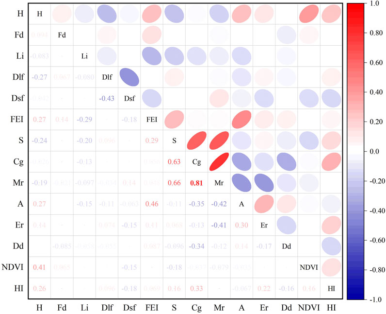
Figure 5. Correlations among the 14 factors.

3.2 Model strategy

In the assessment of debris flow susceptibility, Random Forest (RF) is a widely used and effective machine learning method (Behnia and Blais-Stevens, 2018; Si et al., 2020; Zhang and Wu, 2019). RF is an ensemble learning algorithm based on decision trees, known for its robustness and accuracy in classification and regression tasks. Unlike decision trees, which use a greedy algorithm to build the tree from top to bottom by selecting the best splitting feature and threshold at each node, RF creates each decision tree using bootstrapped samples of the training data, with a random selection of features. This approach ensures diversity among the trees. Each tree independently predicts the outcome for test data, and the final prediction is determined by the majority vote across all trees.

The training process of the Random Forest model can be summarized in three simple steps: 1) For a training set T with N samples and M features, randomly select N samples with replacement to create a training sample D for each tree. The replacement ensures that D maintains N samples, but not all original samples are used; 2) When building a decision tree and a node requires splitting, randomly select m features from the M features in D, where m ≤ M. The optimal splitting strategy is then applied to divide the node, with the process continuing until further splitting is not possible; 3) Repeat steps one to two to build a large number of decision trees, forming the Random Forest.

The ratio between training and test sets influences the performance of the Random Forest model. Increasing the size of the training set generally improves accuracy, but an excessively large training set may lead to a sparse test set, compromising the model’s ability to accurately predict debris flow susceptibility. Most studies adopt a ratio of 7:3 or 8:2. In this study, we used a 7:3 split. Perform grid search to optimize model parameters. Analyzing the performance of the two models will help us assess the impact of freeze-thaw erosion on debris flow susceptibility in the study area.

3.3 Model performance evaluation method

The performance of the models in this study is primarily evaluated using a confusion matrix and the receiver operating characteristic (ROC) curve. The confusion matrix is a fundamental and straightforward method for assessing classification model performance.

Several key performance metrics can be derived from the confusion matrix to quantify the model’s performance across different classes, including Accuracy (Acc), Precision, True Positive Rate (TPR), True Negative Rate (TNR), and False Positive Rate (FPR), as shown in Table 2.

Table 2

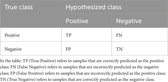
Table 2. Confusion matrix.

Acc: Represents the proportion of correctly classified samples out of the total number of samples. It is calculated as:

$\text{Acc}=\frac{\text{TP}+\text{TN}}{\text{TP}+\text{TN}+\text{FP}+\text{FN}}$

TPR: Indicates the proportion of actual positive samples that are correctly predicted as positive by the model. It is calculated as:

$\text{TPR}=\frac{\text{TP}}{\text{TP}+\text{FN}}$

TNR: Indicates the proportion of actual negative samples that are correctly predicted as negative by the model. It is calculated as:

$\text{TNR}=\frac{\text{TN}}{\text{TN}+\text{FP}}$

FPR: Indicates the proportion of actual negative samples that are incorrectly predicted as positive by the model. It is calculated as:

$\text{FPR}=\frac{\text{FP}}{\text{FP}+\text{TN}}=1-\text{TNR}$

The ROC curve is a tool used to evaluate the performance of classification models and is commonly employed in assessing susceptibility models in machine learning. The curve plots the FPR on the x-axis and the TPR on the y-axis, based on varying probability thresholds from 0 to 1. A ROC curve that is closer to the top-left corner indicates better model performance. The area under the curve (AUC) is used to determine the model’s accuracy. Higher AUC values indicate better accuracy, with values between 0.5 and one considered good (Duan et al., 2023).

4 Results

4.1 Debris flow susceptibility mapping

During the model construction, we trained a 13-factor FEM that included the FEI as one of the features. This model was then compared with a 12-factor NFEM that excluded the FEI to assess the impact of including the FEI on model performance. The debris flow susceptibility index for each watershed unit in the study area, as calculated by both models, was classified into five levels using the Jenks natural breaks method.In FEM, the classification is: Very Low (0–0.44), Low (0.44–0.56), Medium (0.56–0.66), High (0.66–0.75), and Very High (0.75–1). In NFEM, it is: Very Low (0–0.45), Low (0.45–0.56), Medium (0.56–0.65), High (0.65–0.75), Very High (0.75–1). These levels correspond to areas with very low, low, medium, high, and very high susceptibility, respectively. Figure 6 shows the results. Visually, the susceptibility distribution patterns generated by the two models show a high degree of similarity. High and very high susceptibility areas are mainly distributed along both banks of the rivers, with the very high susceptibility zones concentrated in the middle reaches of the Wa River and the lower right bank of the Ma River. Very low and low susceptibility zones are primarily located near the county town of Gongjue and Haga Township. The predictive results of both models align well with field survey data. The primary difference between the two models lies in the proportion of areas classified as high and very low susceptibility zones (Figure 7). The FEM model classifies 63.06% of the area into medium, high, and very high susceptibility zones, while the NFEM model classifies 68.04% into these zones, indicating that the NFEM model tends to overestimate debris flow susceptibility across the study area. In our sample, the proportion of debris flow occurrences is 62.20% (362/582). The proportion of area classified by the FEM model closely matches this observed debris flow occurrence ratio. However, this does not necessarily mean that the FEM outperforms the NFEM, as a close match in area proportions does not imply higher predictive accuracy. Some debris flow-prone areas may be classified as very low or low susceptibility, while areas without debris flow occurrences may be classified as high or very high susceptibility. Such misclassification can affect the overall assessment of the models’ performance, necessitating further analysis to evaluate the predictive accuracy of both models.

Figure 6

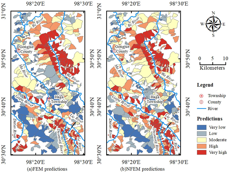
Figure 6. Debris flow susceptibility maps of FEM and NFEM. (a) FEM predictions, (b) NFEM predictions.

Figure 7

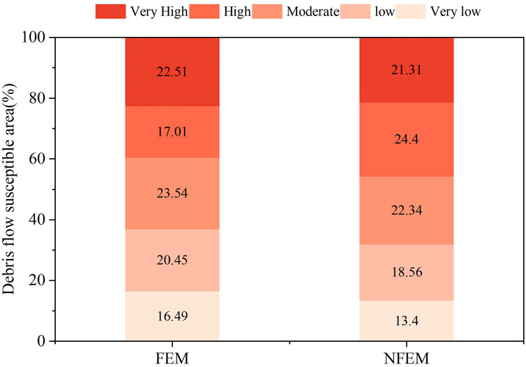
Figure 7. Proportion of susceptibility zones for FEM and NFEM.

4.2 Evaluation of the models

As mentioned earlier, the dataset was divided into training and test sets in a 7:3 ratio to validate the performance of debris flow susceptibility models. ACC, TPR, and TNR were calculated for both models using the training and test datasets (Table 3). These metrics for the training set assess the models’ fit to the study area, while the metrics for the test set evaluate their predictive ability. The results show that the FEM model has higher ACC, TPR, and TNR values on the training set than the NFEM model, indicating that FEM better fits the actual conditions of the study area. Both models exhibit TPR values significantly higher than TNR values, suggesting that they align more closely with positive samples than with negative ones in the study area. In the test dataset, the inclusion of FEI significantly improved the model’s ACC value, increasing from 0.6914 in the NFEM model to 0.7371 in the FEM model, a gain of 0.0457. The TPR values of the two models are similar, with NFEM slightly outperforming FEM. However, FEM’s TNR is substantially higher than that of NFEM, indicating that while their ability to predict positive samples is comparable, FEM has a much stronger ability to predict negative samples. However, it should be noted that both models perform poorly in predicting negative samples; NFEM has a TNR of just 0.3582, while FEM’s TNR is only slightly better than random guessing. This issue may arise from the imbalance in our dataset, where positive samples significantly outnumber negative ones, leading to reduced model learning capacity for negative samples. In summary, the FEM better aligns with the actual conditions of the study area, and the inclusion of FEI effectively enhances the model’s predictive capability.

Table 3

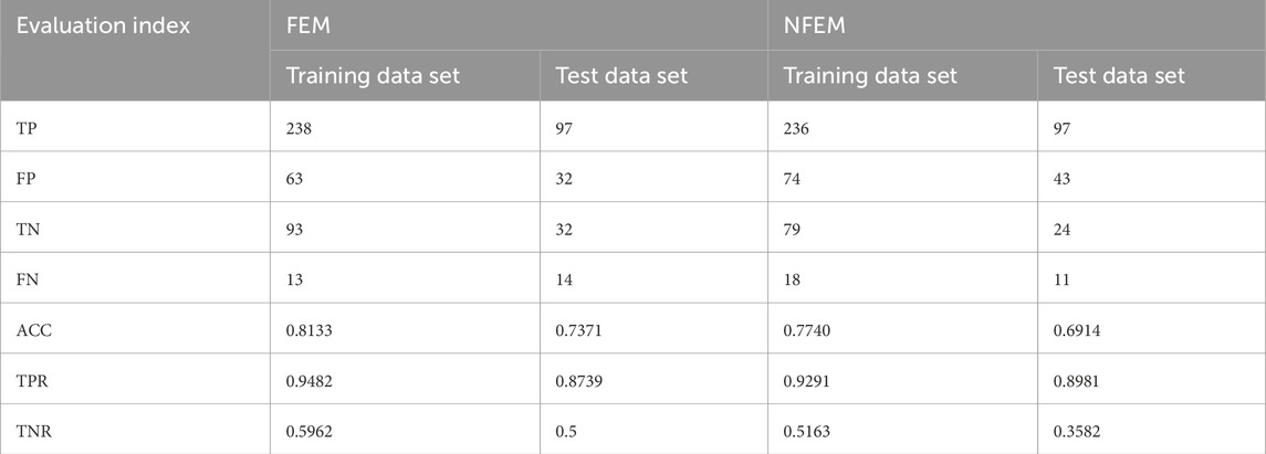
Table 3. Confusion matrix of FEM and NFEM.

To present the data in Table 3 more clearly, we visualized a comparison between the prediction results of the two models and the historical actual situation (Figure 8). Evidently, the discrepancies between the prediction results of both models and the historical actuals for specific watersheds exhibit a striking similarity. Both models predicted that debris flows had occurred in some watersheds where no such events had actually taken place. The core of susceptibility assessment lies in predicting areas and probabilities of future disasters based on the relationship between historical disaster characteristics and environmental conditions. Watersheds with no historical debris flow events might have been identified by the models as highly susceptible due to already possessing conditions conducive to debris flows but lacking triggering factors, or because human activities suppressed the occurrence of debris flows. The causes behind these false positive samples warrant attention and will be further analyzed in the discussion section.

Figure 8

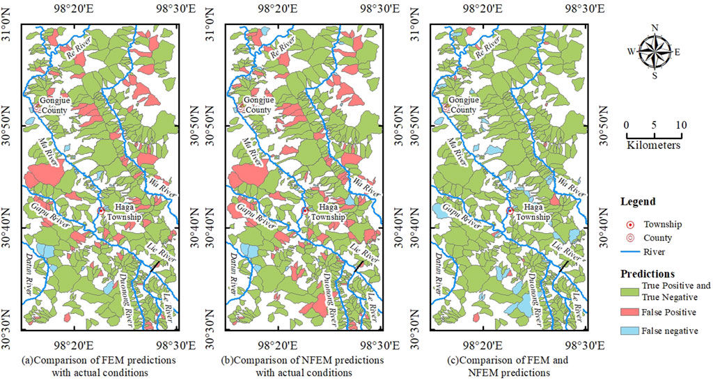
Figure 8. Comparison of FEM and NFEM Prediction Results. (a) Comparison of FEM predictions with actual conditions, (b) Comparison of NFEM predictions with actual conditions, (c) Comparison of FEM predictions with NFEM predictions.

The ROC curve is widely used to evaluate the accuracy of spatial prediction models. The AUC was calculated for both the FEM and NFEM models (Figure 9). Both models achieved an AUC greater than 0.8 on the training dataset, with FEM outperforming NFEM. While the AUC values for the training dataset are high, these values reflect the model’s performance on the training data and are not indicative of overall model performance. The AUC on the test dataset better represents model efficacy. NFEM’s test dataset AUC was 0.6866, indicating poor predictive performance. In contrast, FEM’s AUC increased by approximately 0.06, reaching 0.7407, which is above 0.7, making FEM the better predictive model. This demonstrates that incorporating freeze-thaw erosion intensity as a control factor significantly enhances the accuracy of debris flow susceptibility assessments, aligning better with the regional disaster background.

Figure 9

Figure 9. ROC curves of FEM and NFEM. (a) Training data set, (b) Test data set.

4.3 The importance of controlling factors

The Random Forest model assesses feature importance based on their contribution to the decision tree construction process. This method has the advantages of considering multiple decision trees, being unaffected by feature correlations, and accurately evaluating each feature’s independent contribution. Figure 10 illustrates the factor contribution rates for the FEM and NFEM models. The FEI showed an importance of 7.7%, ranking fifth in the FEM model, indicating a good level of importance. In the NFEM model, excluding FEI, the importance of slope and elevation significantly increased, while factors with high or low importance showed no substantial changes.

Figure 10

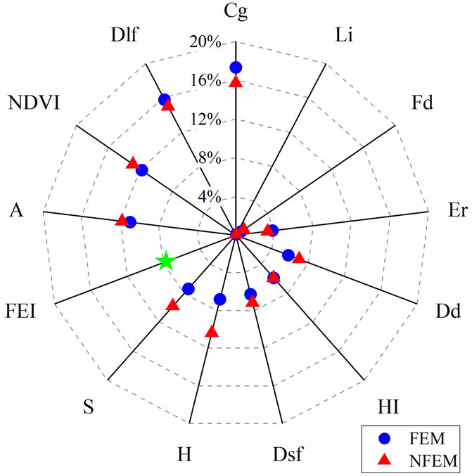
Figure 10. The contribution rate level of factors given by the random forest model.

Regardless of whether FEI is considered, the importance of Cg, Dlf, NDVI, and A is significantly greater than other factors, indicating that these four factors play a critical role in controlling debris flow susceptibility. Cg represents the basic morphological index of the watershed; a higher channel gradient generally increases water velocity and scouring capacity, making loose materials like rock and soil more prone to erosion and transport, thus increasing the likelihood of debris flows. Dlf measures the impact of folding on debris flow susceptibility; the presence of folds usually indicates intense and unstable tectonic movements, leading to significant changes in rock strata, the development of joints and fissures, and the weathering of fragmented rocks, all of which provide material conditions for debris flow outbreaks. NDVI is a commonly used factor for assessing vegetation cover in the study area; vegetation helps slow water flow and absorb rainwater, reducing the impact of water flow during heavy rains. Additionally, vegetation roots help stabilize the soil. An increase in A contributes to more runoff, affecting the occurrence of debris flows. The least important factors in both models are Li and Fd, likely because these control factors are too concentrated in distribution. Most of the watersheds in the area are composed of relatively hard, layered clastic rocks (492 watersheds), with little variation in lithology. Additionally, in 478 out of 582 watersheds, there are no faults, resulting in a fracture density of 0. The overall small differences in these two control factors lead to overly concentrated data, which fails to provide useful information for the model, resulting in their low importance.

5 Discussion

The debris flow susceptibility mapping provided new insights into freeze-thaw erosion-induced debris flows within the study area. Our primary focus was on the reliability of susceptibility mapping that only considers the regional disaster background without including triggering factors, and the change in model prediction accuracy after incorporating the FEI. Based on the results, five key points merit discussion: (1) the causes of false positive samples; (2) the preparation of machine learning datasets; (3) the selection of control factors; (4) the importance of control factors and model accuracy; (5) the mechanism analysis on the improvement of model performance by FEI.

5.1 Causes of false positive samples

The random forest model does not provide a clear process for making predictions like the decision tree algorithm does (Wu et al., 2024). Therefore, analyzing the causes of false positive samples predicted by the two models requires returning to the data itself for analysis. Thus, we selected the watersheds identified as false positives by both models, as shown in Figure 8, for further analysis. We identified three main reasons for these errors:

1.The channel acts as a transport pathway for debris flows, and its morphology significantly influences debris flow development. In both models, channel gradient is identified as the most important factor. We found that watersheds with false positive samples generally have larger areas and longer channel lengths. Above the mountain outlets, the channel gradients show significant variability, exhibiting a “steep-gentle” transition (Figure 11a), which facilitates the accumulation of loose materials at these transitional terrains. Downstream of the mountain outlets, the channel gradients are very gentle, resulting in poor transport capacity. Additionally, we observed that these watersheds often have meandering and irregular downstream channels (Figure 11b), which are unfavorable for debris flow development.Although such terrain restricts the movement of debris flows, it also causes a large amount of loose materials to accumulate in the upstream channel. Under certain triggering factors, the possibility of debris flow outbreaks is high, so it is judged as highly susceptible by the models.

2.Some watersheds exhibit significant human activities, such as villages, roads, and agricultural fields (Figures 11b,c). The existence of human activities has led to certain engineering modifications in the watershed, temporarily suppressing the occurrence of debris flows. However, as artificially planted vegetation degenerates or engineering works age, the inhibitory effect may be lost in the future. In fact, the models’ prediction of high susceptibility indicates potential risks.

3.The FEI control factor we introduced is directly related to the thickness of the surface humus layer. In these watersheds, the layer is quite thin (Figure 11d), and the freeze-thaw erosion is relatively weak, leading to limited sources of loose materials in the current watersheds, so no debris flows have occurred. However, over time, repeated freeze-thaw erosion will break the rock and soil mass, making the possibility of debris flow outbreaks high.

Figure 11

Figure 11. Analysis of the causes of error in the watershed. (a) The variation of the longitudinal gradient of the main channel in the watershed. (b) Channel curvature and human engineering activities. (c) Human engineering activities. (d) Thin thickness of the cover layer.

5.2 Preparation of machine learning dataset

Currently, researchers are more focused on obtaining positive samples when preparing machine learning datasets. Negative samples are typically selected randomly, which, while effective in most cases, risks including unidentified actual debris flow samples, potentially skewing the classification of positive samples. Therefore, we used the same method for selecting negative samples as for positive ones. However, due to constraints, the number of negative samples we obtained was much smaller than that of positive samples, leading to the model’s poor learning ability for negative samples. Nonetheless, both models still achieved high accuracy, which can be attributed to their excellent predictive power for positive samples. These results suggest that the debris flow dataset we developed is representative and can be considered a reliable tool for debris flow susceptibility assessment. However, in future research, we plan to address the imbalance in positive and negative samples by expanding the study area and acquiring higher-resolution satellite images.

5.3 Selection of control factors

There is no standardized guideline for selecting control factors in debris flow susceptibility assessments using machine learning. However, a general consensus has emerged: control factors should be chosen by considering both the fundamental mechanisms of debris flow and the specific conditions of the study area. Reichenbach et al. (Reichenbach et al., 2018) colleagues conducted a critical review of 565 articles on landslide susceptibility assessments published between 1983 and 2016. These studies included various landslide types, such as “debris flows” and “mudflows”. They found that most studies used factors related to terrain morphology, with researchers preferring simple and straightforward parameters like elevation, relief, slope, aspect, and curvature. We also analyzed control factors, but our study focused explicitly on the topics of “debris flow” and “machine learning”, which led to a smaller number of articles compared to Reichenbach’s review. Our analysis is largely consistent with their findings. Terrain-related factors are the most commonly used, with researchers favoring simple and direct control factors such as elevation, slope, and aspect. These simple control factors can be easily derived from Digital Elevation Models (DEM) using modern Geographic Information Systems (GIS). More complex factors, such as the TWI and roughness, have also proven effective in susceptibility assessments. However, these complex terrain factors are typically derived from simple factors like elevation, slope, and area through mathematical processing. It remains unclear whether using both simple factors and the complex factors derived from them simultaneously in susceptibility assessments affects model performance or the importance of control factors. Current control factor selection tends to focus on analyzing correlations between factors from a data perspective, with less emphasis on their physical meaning or influence on debris flow. Thus, developing a standard for selecting control factors with minimal statistical and physical correlation remains a topic requiring further research.

Expert judgment is essential when selecting factors, making it crucial to consider the geological conditions of the study area. An analysis of common factors shows that the same factor may behave very differently across regions with varying geological backgrounds. In selecting factors, we accounted for the significant freeze-thaw erosion that fractures the rock and soil in our study area by introducing a method for quantitatively estimating freeze-thaw erosion intensity. Di et al. (2019), in assessing debris flow susceptibility in Sichuan Province, introduced freeze-thaw erosion intensity as a factor, categorizing it into four levels: Very low, Low, Moderate, and High. Compared to qualitative assessments, our quantitative approach is more specific and intuitive. When assessing debris flow susceptibility in cold mountainous regions, freeze-thaw erosion, in addition to wind and water erosion, cannot be overlooked.

5.4 The importance of control factors and model accuracy

A comprehensive analysis of model accuracy and factor importance revealed that freeze-thaw erosion plays a critical role in controlling debris flow susceptibility in the study area. Research by Zhang and Wu (2019) demonstrated that key control factors determine a model’s baseline predictive ability. Removing important factors leads to an irreversible decline in predictive performance, while removing unimportant factors can improve the model. After removing FEI, our model’s accuracy dropped by 0.457, and the AUC decreased by 0.0541. FEI is one of the key control factors that determine the model’s baseline predictive ability. The ranking of original control factors did not change significantly, indicating that debris flow occurrence in the study area is strongly related to factors such as Cg, Dlf, NDVI, and area. The low contribution of fracture density and lithology is primarily due to the limited amount of useful information these factors provide; the model can hardly extract effective susceptibility-related data from fracture density and rock group types.

Models that account for freeze-thaw erosion have achieved high accuracy and predictive performance. However, there is a significant difference in AUC values between the training set and test set for the FEM, indicating certain limitations in the model’s generalization ability. Such a gap is common in machine learning applications for geological hazard assessment with small samples and high heterogeneity. We attribute this discrepancy in the FEM to three reasons. First, since we randomly split the entire dataset into training and test sets at a 7:3 ratio, the small sample size of the test set may fail to fully represent the overall geological condition variability of the study area. Second, although the random forest model has a certain effect in suppressing overfitting, it may still overfit when “local features” exist in the test set, and the insufficient number of negative samples leads to inadequate learning of negative sample features. Third, the complex terrain of the study area, along with significant spatial variations in factors such as freeze-thaw erosion intensity and vegetation coverage, further affect the prediction accuracy. To address these three issues, future efforts can expand the sample size by enlarging the study area and divide samples proportionally according to factor distributions, ensuring that the training and test sets have more consistent factor distributions and reducing distribution bias. We will continue research and conduct field surveys to expand the sample size to improve this situation.

In summary, the AUC gap between the training set and test set reflects the typical challenges in model evaluation for small-sample, high-heterogeneity regions, with the core reason being a mismatch between data distribution differences and model generalization ability. While this phenomenon does not negate the superiority of the FEM model, it reminds us that in practical applications, we should focus on “high susceptibility - historically no disaster” areas in combination with field verification and avoid directly relying on model results for decision-making.

5.5 Mechanism analysis on the improvement of model performance by FEI

The significant improvement in model performance after introducing FEI in this study is no coincidence. It is determined by the physical meaning of FEI, the geological background of the study area, and its in-depth connection with the debris flow formation mechanism, which can be elaborated from the following two aspects.

5.5.1 FEI accurately reflects the unique material supply mechanism in the study area

The study area is located in the high-altitude region of the eastern Tibetan Plateau, where the temperature difference between day and night is large and permafrost is well-developed. Freeze-thaw cycles are the dominant process for the fragmentation of rock and soil masses (Figures 2a,b). Field investigations have confirmed that the loose debris material generated by freeze-thaw erosion is the most important material source for debris flows. By quantifying factors such as the thickness of surface humus, slope, and elevation, FEI directly characterizes the damage intensity of freeze-thaw action on rock and soil masses. A comparison between the distribution of debris flow watersheds in the study area (Figure 2c) and the FEI values of each watershed (Figure 12f) reveals that areas with high FEI values (such as the middle reaches of the Wa River) correspond to surface lithological fracture zones caused by frequent freeze-thaw, where there are sufficient reserves of loose debris material, highly consistent with the areas with high incidence of debris flows. In areas with low FEI values (such as the vicinity of Gongjue County), freeze-thaw action is weak, the rock and soil masses are highly intact, and material sources are scarce, resulting in a low incidence of debris flows. In contrast, the NFEM model only relies on conventional factors such as slope and lithology, and cannot identify the phenomenon of high content of loose debris material in the watershed caused by freeze-thaw erosion, leading to misjudgments by the model.

Figure 12

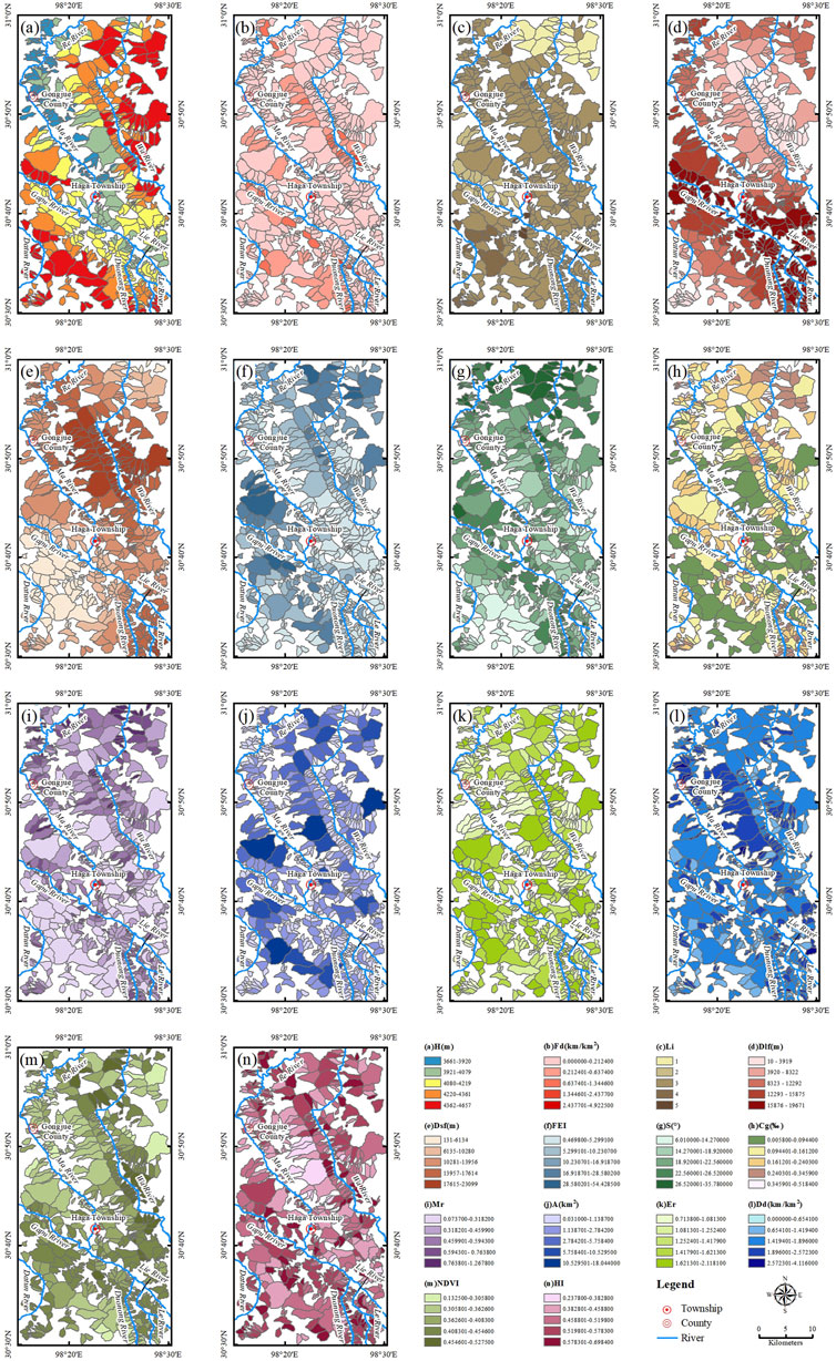
Figure 12. The controlling factors. (a) H, (b) Fd, (c) Li, (d) Dlf, (e) Dsf, (f) FEI, (g) S, (h) Cg, (i) Mr, (j) A, (k) Er, (l) Dd, (m) NDVI, (n) HI.

5.5.2 FEI makes up for the neglect of freeze-thaw-hydrological coupling processes by conventional factors

The formation of debris flows requires the synergistic effect of material sources, dynamic forces, and hydrological conditions. Freeze-thaw erosion not only provides material sources but also affects hydrological responses by changing the permeability of rock and soil masses: fractures generated by freeze-thaw can enhance the infiltration capacity of surface water, accelerating the saturation rate of loose debris material, which are thus more likely to be mobilized by water flow. Factors such as slope aspect and shrub coverage included in FEI indirectly reflect the impact of solar radiation intensity on freeze-thaw frequency and the role of vegetation in soil and water conservation, thereby quantifying the coupling relationship between material supply and hydrological dynamics. This explains why the predictive ability of FEM for negative samples is significantly higher than that of NFEM. For areas with steep slopes but low FEI values (such as shady slopes with dense vegetation), FEI can identify the dual inhibitory effects of insufficient loose debris material and soil consolidation by vegetation on debris flow outbreaks, avoiding misjudgments.

In summary, the inclusion of FEI is not simply the addition of a variable. Instead, by accurately characterizing the dominant freeze-thaw erosion processes in the study area, it fills the gap in the adaptability of conventional factors to special geological environments, making the model more consistent with the physical mechanisms of regional disaster formation and thus achieving better predictive performance. This result confirms that in high-altitude mountainous areas with significant freeze-thaw effects, the freeze-thaw erosion factor should serve as a core controlling factor in the assessment of debris flow susceptibility.

6 Conclusion

Our study on the susceptibility of freeze-thaw erosion induced debris flow in the east of Tibetan Plateau has led to the following main conclusions.

1. When evaluating the predictive ability of control factors, the variability in their statistical importance was significant. This indicates substantial differences in the contribution levels of different control factors across various models, which is likely due to the distinct geological conditions of different study areas. Elevation was the highest-ranked factor on average and exhibited the least variability, suggesting that elevation is strongly associated with debris flow occurrences in the majority of study areas.

2. In evaluating the susceptibility to debris flows using machine learning, we propose a new factor selection strategy consisting of two steps. The first step involves identifying key controlling factors by considering three conditions that contribute to debris flow development: material source conditions, dynamic conditions, and hydrological conditions. These factors are selected based on their high occurrence and strong performance in existing machine learning susceptibility evaluation models. The second step introduces critical controlling factors into the model, informed by the mechanisms of debris flow formation. In this study, we consider the freeze-thaw erosion intensity as a crucial controlling factor for freeze-thaw erosion induced debris flow, as it governs the material source for these flows and affects the frequency, triggering conditions, and scale of the disasters. This new factor selection strategy offers significant advantages by ensuring the accessibility of controlling factors while aligning with the actual geological conditions of the study area, thereby enhancing the interpretability of the assessment results.

3. The accuracy of FEM considering freeze-thaw erosion is 0.7371, and the AUC value is 0.7407, which is higher than NFEM’s 0.6914 and 0.6866. The proportion of areas classified as “high” and “medium” susceptibility decreased, resulting in predictions that better aligned with the actual distribution of debris flows. Therefore, we conclude that freeze-thaw erosion plays a crucial role in assessing debris flow susceptibility in the study area and should be taken into account.

Data availability statement

The raw data supporting the conclusions of this article will be made available by the authors, without undue reservation.

Author contributions

YY: Conceptualization, Data curation, Methodology, Software, Writing – original draft, Writing – review and editing. YZ: Data curation, Visualization, Writing – original draft, Writing – review and editing. HH: Conceptualization, Funding acquisition, Methodology, Resources, Writing – review and editing. JZ: Investigation, Visualization, Writing – review and editing. QL: Investigation, Visualization, Writing – review and editing. JP: Supervision, Validation, Writing – review and editing.

Funding

The author(s) declare that financial support was received for the research and/or publication of this article. This study was funded by Major Science and Technology Project of Northwest Engineering Corporation Limited (XBY-ZDKJ-2023-9).

Acknowledgments

The authors would like to thank all the staff members of the Investigation and Evaluation Office of the Institute of Exploration Technology for providing valuable and detailed on-site information during the field investigation.

Conflict of interest

The authors declare that the research was conducted in the absence of any commercial or financial relationships that could be construed as a potential conflict of interest.

The authors declare that this study received funding from Northwest Engineering Corporation Limited. The funder had the following involvement in the study: assisting in carrying out field investigation work and providing suggestions on research ideas.

Generative AI statement

The author(s) declare that no Generative AI was used in the creation of this manuscript.

Any alternative text (alt text) provided alongside figures in this article has been generated by Frontiers with the support of artificial intelligence and reasonable efforts have been made to ensure accuracy, including review by the authors wherever possible. If you identify any issues, please contact us.

Publisher’s note

All claims expressed in this article are solely those of the authors and do not necessarily represent those of their affiliated organizations, or those of the publisher, the editors and the reviewers. Any product that may be evaluated in this article, or claim that may be made by its manufacturer, is not guaranteed or endorsed by the publisher.

References

Achour, Y., Garçia, S., and Cavaleiro, V. (2018). Gis-based spatial prediction of debris flows using logistic regression and frequency ratio models for zêzere river basin and its surrounding area, northwest covilhã, Portugal. Arabian J. Geosciences 11, 550. doi:10.1007/s12517-018-3920-9

CrossRef Full Text | Google Scholar

Behnia, P., and Blais-Stevens, A. (2018). Landslide susceptibility modelling using the quantitative random forest method along the northern portion of the Yukon Alaska highway corridor, Canada. Nat. Hazards 90, 1407–1426. doi:10.1007/s11069-017-3104-z

CrossRef Full Text | Google Scholar

Bregoli, F., Medina, V., Chevalier, G., Hürlimann, M., and Bateman, A. (2015). Debris-flow susceptibility assessment at regional scale: validation on an alpine environment. Landslides 12, 437–454. doi:10.1007/s10346-014-0493-x

CrossRef Full Text | Google Scholar

Cao, J., Zhang, Z., Du, J., Zhang, L., Song, Y., and Sun, G. (2020). Multi-geohazards susceptibility mapping based on machine learning—a case study in Jiuzhaigou, China. Nat. Hazards 102, 851–871. doi:10.1007/s11069-020-03927-8

CrossRef Full Text | Google Scholar

Cao, J., Qin, S., Yao, J., Zhang, C., Liu, G., Zhao, Y., et al. (2023). Debris flow susceptibility assessment based on information value and machine learning coupling method: from the perspective of sustainable development. Environ. Sci. Pollut. Res. 30, 87500–87516. doi:10.1007/s11356-023-28575-w

PubMed Abstract | CrossRef Full Text | Google Scholar

Chen, X., Chen, H., You, Y., and Liu, J. (2015). Susceptibility assessment of debris flows using the analytic hierarchy process method − a case study in subao river valley, China. J. Rock Mech. Geotechnical Eng. 7, 404–410. doi:10.1016/j.jrmge.2015.04.003

CrossRef Full Text | Google Scholar

Chen, M., Chang, M., Xu, Q., Tang, C., Dong, X., and Li, L. (2024a). Identifying potential debris flow hazards after the 2022 mw 6.8 Luding earthquake in southwestern China. Bull. Eng. Geol. Environ. 83, 241. doi:10.1007/s10064-024-03749-z

CrossRef Full Text | Google Scholar

Chen, Z., Quan, H., Jin, R., Lin, Z., and Jin, G. (2024b). Debris flow susceptibility assessment based on boosting ensemble learning techniques: a case study in the Tumen River basin, China. Stoch. Environ. Res. Risk Assess. 38, 2359–2382. doi:10.1007/s00477-024-02683-6

CrossRef Full Text | Google Scholar

Di, B., Zhang, H., Liu, Y., Li, J., Chen, N., Stamatopoulos, C. A., et al. (2019). Assessing susceptibility of debris flow in southwest China using gradient boosting machine. Sci. Rep. 9, 12532. doi:10.1038/s41598-019-48986-5

PubMed Abstract | CrossRef Full Text | Google Scholar

Dong, A.-j., and Wu, C.-x. (2022). Evaluation of debris flow susceptibility in Leibo county based on GIS and FNN-SGD. Softw. Guide 21, 58–68. doi:10.11907/rjdk.212560

CrossRef Full Text | Google Scholar

Duan, Y., Luo, J., Pei, X., and Liu, Z. (2023). Co-seismic landslides triggered by the 2014 mw 6.2 ludian earthquake, yunnan, China: spatial distribution, directional effect, and controlling factors. Remote Sens. 15, 4444. doi:10.3390/rs15184444

CrossRef Full Text | Google Scholar

Elkadiri, R., Sultan, M., Youssef, A. M., Elbayoumi, T., Chase, R., Bulkhi, A. B., et al. (2014). A remote sensing-based approach for debris-flow susceptibility assessment using artificial neural networks and logistic regression modeling. IEEE J. Sel. Top. Appl. Earth Observations Remote Sens. 7, 4818–4835. doi:10.1109/JSTARS.2014.2337273

CrossRef Full Text | Google Scholar

Gao, R.-y., Wang, C.-m., and Liang, Z. (2021). Comparison of different sampling strategies for debris flow susceptibility mapping: a case study using the centroids of the scarp area, flowing area and accumulation area of debris flow watersheds. J. Mt. Sci. 18, 1476–1488. doi:10.1007/s11629-020-6471-y

CrossRef Full Text | Google Scholar

Gu, F., Chen, J., Sun, X., Li, Y., Zhang, Y., and Wang, Q. (2023). Comparison of machine learning and traditional statistical methods in debris flow susceptibility assessment: a case study of Changping district, Beijing. Water 15, 705. doi:10.3390/w15040705

CrossRef Full Text | Google Scholar

Guzzetti, F., Carrara, A., Cardinali, M., and Reichenbach, P. (1999). Landslide hazard evaluation: a review of current techniques and their application in a multi-scale study, central Italy. Geomorphology 31, 181–216. doi:10.1016/S0169-555X(99)00078-1

CrossRef Full Text | Google Scholar

Huang, H., Tian, Y., Liu, J., Zhang, J., Yang, D., and Yang, S. (2021). The mechanism and sensitivity analysis of soil freeze-thaw erosion on slope in eastern Tibet. ACTA Geogr. SIN. 76, 87–100. doi:10.11821/dlxb202101007

CrossRef Full Text | Google Scholar

Huang, H., Wang, Y., Li, Y., Zhou, Y., and Zeng, Z. (2022). Debris-flow susceptibility assessment in China: a comparison between traditional statistical and machine learning methods. Remote Sens. 14, 4475. doi:10.3390/rs14184475

CrossRef Full Text | Google Scholar

Kumar, A., and Sarkar, R. (2023). Debris flow susceptibility evaluation—a review. Iran. J. Sci. Technol. Trans. Civ. Eng. 47, 1277–1292. doi:10.1007/s40996-022-01000-x

CrossRef Full Text | Google Scholar

Lay, U. S., Pradhan, B., Yusoff, Z. B. M., Abdallah, A. F. B., Aryal, J., and Park, H.-J. (2019). Data mining and statistical approaches in debris-flow susceptibility modelling using airborne lidar data. Sensors 19, 3451. doi:10.3390/s19163451

PubMed Abstract | CrossRef Full Text | Google Scholar

Li, J., and Lv, Y. (2022). Risk assessment of debris flow in Huyugou river basin based on machine learning and mass flow. Mob. Inf. Syst. 2022, 1–10. doi:10.1155/2022/9751504

CrossRef Full Text | Google Scholar

Li, Y., Chen, W., Rezaie, F., Rahmati, O., Davoudi Moghaddam, D., Tiefenbacher, J., et al. (2022). Debris flows modeling using geo-environmental factors: developing hybridized deep-learning algorithms. Geocarto Int. 37, 5150–5173. doi:10.1080/10106049.2021.1912194

CrossRef Full Text | Google Scholar

Li, K., Zhao, J., and Lin, Y. (2023). Debris-flow susceptibility assessment in Dongchuan using stacking ensemble learning including multiple heterogeneous learners with rfe for factor optimization. Nat. Hazards 118, 2477–2511. doi:10.1007/s11069-023-06099-3

CrossRef Full Text | Google Scholar

Li, Y., Jiang, W., Feng, X., Lv, S., Yu, W., and Ma, E. (2024). Debris flow susceptibility mapping in alpine canyon region: a case study of Nujiang prefecture. Bull. Eng. Geol. Environ. 83, 169. doi:10.1007/s10064-024-03657-2

CrossRef Full Text | Google Scholar

Liang, W.-j., Zhuang, D.-f., Jiang, D., Pan, J.-j., and Ren, H.-y. (2012). Assessment of debris flow hazards using a bayesian network. Geomorphology 171-172, 94–100. doi:10.1016/j.geomorph.2012.05.008

CrossRef Full Text | Google Scholar

Liang, Z., Wang, C.-M., Zhang, Z.-M., and Khan, K.-U.-J. (2020). A comparison of statistical and machine learning methods for debris flow susceptibility mapping. Stoch. Environ. Res. Risk Assess. 34, 1887–1907. doi:10.1007/s00477-020-01851-8

CrossRef Full Text | Google Scholar

Liang, X., Ge, Y., Zeng, L., Lyu, L., Sun, Q., Sun, Y., et al. (2023). Debris flow susceptibility based on the connectivity of potential material sources in the Dadu river basin. Eng. Geol. 312, 106947. doi:10.1016/j.enggeo.2022.106947

CrossRef Full Text | Google Scholar

Liu, K., Wang, M., Cao, Y., Zhu, W., and Yang, G. (2018). Susceptibility of existing and planned Chinese railway system subjected to rainfall-induced multi-hazards. Transp. Res. Part A Policy Pract. 117, 214–226. doi:10.1016/j.tra.2018.08.030

CrossRef Full Text | Google Scholar

Liu, Y., Chen, J., Sun, X., Li, Y., Zhang, Y., Xu, W., et al. (2024). A progressive framework combining unsupervised and optimized supervised learning for debris flow susceptibility assessment. CATENA 234, 107560. doi:10.1016/j.catena.2023.107560

CrossRef Full Text | Google Scholar

Lv, J., Qin, S., Chen, J., Qiao, S., Yao, J., Zhao, X., et al. (2023). Application of different watershed units to debris flow susceptibility mapping: a case study of northeast China. Front. Earth Sci. 11, 1118160. doi:10.3389/feart.2023.1118160

CrossRef Full Text | Google Scholar

Melton, M. A. (1966). The geomorphic and paleoclimatic significance of alluvial deposits in southern Arizona: a reply. J. Geol. 74, 102–106. doi:10.1086/627147

CrossRef Full Text | Google Scholar

Nefeslioglu, H. A., Gokceoglu, C., and Sonmez, H. (2008). An assessment on the use of logistic regression and artificial neural networks with different sampling strategies for the preparation of landslide susceptibility maps. Eng. Geol. 97, 171–191. doi:10.1016/j.enggeo.2008.01.004

CrossRef Full Text | Google Scholar

Pitscheider, F., Steger, S., Cavalli, M., Comiti, F., and Scorpio, V. (2024). Areas simultaneously susceptible and (dis-)connected to debris flows in the Dolomites (Italy): regional-scale application of a novel data-driven approach. J. Maps 20, 1–14. doi:10.1080/17445647.2024.2307549

CrossRef Full Text | Google Scholar

Ponziani, M., Ponziani, D., Giorgi, A., Stevenin, H., and Ratto, S. M. (2023). The use of machine learning techniques for a predictive model of debris flows triggered by short intense rainfall. Nat. Hazards 117, 143–162. doi:10.1007/s11069-023-05853-x

CrossRef Full Text | Google Scholar

Pourghasemi, H. R., and Rahmati, O. (2018). Prediction of the landslide susceptibility: which algorithm, which precision? CATENA 162, 177–192. doi:10.1016/j.catena.2017.11.022

CrossRef Full Text | Google Scholar

Qin, S., Qiao, S., Yao, J., Zhang, L., Liu, X., Guo, X., et al. (2022). Establishing a GIS-based evaluation method considering spatial heterogeneity for debris flow susceptibility mapping at the regional scale. Nat. Hazards 114, 2709–2738. doi:10.1007/s11069-022-05487-5

CrossRef Full Text | Google Scholar

Qing, F., Zhao, Y., Meng, X., Su, X., Qi, T., and Yue, D. (2020). Application of machine learning to debris flow susceptibility mapping along the China–Pakistan Karakoram highway. Remote Sens. 12, 2933. doi:10.3390/rs12182933

CrossRef Full Text | Google Scholar

Qiu, C., Su, L., Zou, Q., and Geng, X. (2022). A hybrid machine-learning model to map glacier-related debris flow susceptibility along Gyirong Zangbo watershed under the changing climate. Sci. Total Environ. 818, 151752. doi:10.1016/j.scitotenv.2021.151752

PubMed Abstract | CrossRef Full Text | Google Scholar

Reichenbach, P., Rossi, M., Malamud, B. D., Mihir, M., and Guzzetti, F. (2018). A review of statistically-based landslide susceptibility models. Earth-Science Rev. 180, 60–91. doi:10.1016/j.earscirev.2018.03.001

CrossRef Full Text | Google Scholar

Rupert, M. G., Cannon, S. H., Gartner, J. E., Michael, J. A., and Helsel, D. R. (2008). Using logistic regression to predict a probability of debris flows in areas burned by wildfires, southern California, 2003-2006. Open-File Report.

Google Scholar

Schumm, S. A. (1956). Evolution of drainage systems and slopes in badlands at Perth Amboy, New Jersey. GSA Bulletin 67, 597–646. doi:10.1130/0016-7606(1956)67[597:Eodsas]2.0.Co;2

CrossRef Full Text | Google Scholar

Si, A., Zhang, J., Zhang, Y., Kazuva, E., Dong, Z., Bao, Y., et al. (2020). Debris flow susceptibility assessment using the integrated random forest based steady-state infinite slope method: a case study in Changbai mountain, China. China. Water 12, 2057. doi:10.3390/w12072057

CrossRef Full Text | Google Scholar

Strahler, A. N. (1952). Hypsometric (area-altitude) analysis of erosional topography. GSA Bull. 63, 1117–1142. doi:10.1130/0016-7606(1952)63[1117:Haaoet]2.0.Co;2

CrossRef Full Text | Google Scholar

Sun, X., Yu, C., Li, Y., and Rene, N. N. (2022). Susceptibility mapping of typical geological hazards in Helong city affected by volcanic activity of Changbai mountain, northeastern China. ISPRS Int. J. Geo-Information 11, 344. doi:10.3390/ijgi11060344

CrossRef Full Text | Google Scholar

Ullah, K., Wang, Y., Fang, Z., Wang, L., and Rahman, M. (2022). Multi-hazard susceptibility mapping based on convolutional neural networks. Geosci. Front. 13, 101425. doi:10.1016/j.gsf.2022.101425

CrossRef Full Text | Google Scholar

Wang, J., Yu, Y., Yang, S., Lu, G.-h., and Ou, G.-q. (2014). A modified certainty coefficient method (m-cf) for debris flow susceptibility assessment: a case study for the Wenchuan earthquake meizoseismal areas. J. Mt. Sci. 11, 1286–1297. doi:10.1007/s11629-013-2781-7

CrossRef Full Text | Google Scholar

Wang, Q., Wang, C., Tang, H., Wu, D., and Wang, F. (2024). Semi-supervised deep learning based on label propagation algorithm for debris flow susceptibility assessment in few-label scenarios. Stoch. Environ. Res. Risk Assess. 38, 2875–2890. doi:10.1007/s00477-024-02719-x

CrossRef Full Text | Google Scholar

Wu, S., Chen, J., Zhou, W., Iqbal, J., and Yao, L. (2019). A modified logit model for assessment and validation of debris-flow susceptibility. Bull. Eng. Geol. Environ. 78, 4421–4438. doi:10.1007/s10064-018-1412-5

CrossRef Full Text | Google Scholar

Wu, B., Shi, Z., Zheng, H., Peng, M., and Meng, S. (2024). Impact of sampling for landslide susceptibility assessment using interpretable machine learning models. Bull. Eng. Geol. Environ. 83, 461. doi:10.1007/s10064-024-03980-8

CrossRef Full Text | Google Scholar

Xiong, K., Adhikari, B. R., Stamatopoulos, C. A., Zhan, Y., Wu, S., Dong, Z., et al. (2020). Comparison of different machine learning methods for debris flow susceptibility mapping: a case study in the Sichuan province, China. Remote Sens. 12, 295. doi:10.3390/rs12020295

CrossRef Full Text | Google Scholar

Xu, F., and Wang, B. (2022). Debris flow susceptibility mapping in mountainous area based on multi-source data fusion and cnn model – taking Nujiang prefecture, China as an example. Int. J. Digital Earth 15, 1966–1988. doi:10.1080/17538947.2022.2142304

CrossRef Full Text | Google Scholar

Xu, W., Yu, W., Jing, S., Zhang, G., and Huang, J. (2013). Debris flow susceptibility assessment by gis and information value model in a large-scale region, sichuan province (China). Nat. Hazards 65, 1379–1392. doi:10.1007/s11069-012-0414-z

CrossRef Full Text | Google Scholar

Yanting, H., and Yonggang, G. (2023). Risk assessment of rain-induced debris flow in the lower reaches of Yajiang river based on gis and cf coupling models. Open Geosci. 15. 20220472. doi:10.1515/geo-2022-0472

CrossRef Full Text | Google Scholar

Zhang, S., and Wu, G. (2019). Debris flow susceptibility and its reliability based on random forest and GIS. Earth Sci. 44, 3115–3134. doi:10.3799/dqkx.2019.081

CrossRef Full Text | Google Scholar

Zhang, Y., Ge, T., Tian, W., and Liou, Y.-A. (2019). Debris flow susceptibility mapping using machine-learning techniques in Shigatse area, China. Remote Sens. 11, 2801. doi:10.3390/rs11232801

CrossRef Full Text | Google Scholar

Zhang, Y., Chen, J., Wang, Q., Tan, C., Li, Y., Sun, X., et al. (2022). Geographic information system models with fuzzy logic for susceptibility maps of debris flow using multiple types of parameters: a case study in Pinggu district of Beijing, China. Nat. Hazards Earth Syst. Sci. 22, 2239–2255. doi:10.5194/nhess-22-2239-2022

CrossRef Full Text | Google Scholar

Zhao, Y., Meng, X., Qi, T., Qing, F., Xiong, M., Li, Y., et al. (2020). Ai-based identification of low-frequency debris flow catchments in the Bailong river basin, China. Geomorphology 359, 107125. doi:10.1016/j.geomorph.2020.107125

CrossRef Full Text | Google Scholar

Zhao, H., Wei, A., Ma, F., Dai, F., Jiang, Y., and Li, H. (2024). Comparison of debris flow susceptibility assessment methods: support vector machine, particle swarm optimization, and feature selection techniques. J. Mt. Sci. 21, 397–412. doi:10.1007/s11629-023-8395-9

CrossRef Full Text | Google Scholar

Zhou, Y., Yue, D., Liang, G., Li, S., Zhao, Y., Chao, Z., et al. (2022). Risk assessment of debris flow in a mountain-basin area, western China. Remote Sens. 14, 2942. doi:10.3390/rs14122942

CrossRef Full Text | Google Scholar

Zhou, J., Huang, J., Sun, Z., Yi, Q., and He, A. (2024). Machine learning approaches to debris flow susceptibility analyses in the Yunnan section of the Nujiang river basin. PeerJ 12, e17352. doi:10.7717/peerj.17352

PubMed Abstract | CrossRef Full Text | Google Scholar

Zhu, A. X., Miao, Y., Liu, J., Bai, S., Zeng, C., Ma, T., et al. (2019). A similarity-based approach to sampling absence data for landslide susceptibility mapping using data-driven methods. CATENA 183, 104188. doi:10.1016/j.catena.2019.104188

CrossRef Full Text | Google Scholar