Uncertainty-quantified 3D ambient noise tomography using transdimensional Monte Carlo inversion

Traditional two-step surface-wave tomography often yields discontinuous models and compound uncertainty. We present the first fully 3-D transdimensional Bayesian inversion with adaptive Voronoi parameterization and reversible-jump MCMC for near-surface engineering-scale arrays, providing voxel-level uncertainty estimates. From 1 week of ambient-noise records acquired by a 101-station linear array (120 m spacing) across the F1 fault zone, we extracted phase velocities via frequency–wavenumber analysis of Rayleigh waves (0.5–3 s). The resulting 3-D Vs. model reveals (i) 300–800 m s^-1 in the upper 50 m, (ii) 2.1 ± 0.05 km s^-1 at 0–1 km, (iii) 2.6–2.9 ± 0.08 km s^-1 at 1–3 km, and (iv) 2.8–3.1 ± 0.12 km s^-1 at 3–5 km beneath the fault trace. Voxel-wise 1σ uncertainties range from <5% in the shallowest 2 km to 12% at 5 km depth. These Vs. values and their uncertainties can be directly converted to engineering mechanical parameters: shear modulus G = ρVs², Young’s modulus E = 2G (1+ν), and Poisson’s ratio ν, enabling quantitative assessment of excavation stability, tunnel lining design, and slope stability across the F1 fault zone. The 3-D Bayesian framework mitigates over-fitting biases inherent in sequential inversions and offers critical, uncertainty-aware constraints for multi-stage tectonic reconstruction of the North China Craton destruction belt.

1 Introduction

Seismic tomography serves as a fundamental technique for developing 3D models of Earth’s interior structure. Contemporary approaches predominantly utilize surface waves for imaging purposes. These seismic waves propagate along crustal boundaries where abrupt changes in physical properties commonly occur, with their oscillation depths being frequency-dependent (Aki and Richards, 1980). The dispersive nature of surface waves manifests through distinct propagation velocities at different frequencies, each velocity corresponding to specific subsurface depth sensitivities. This dispersion characteristic enables multi-scale tomographic investigations through velocity measurements, including regional-scale analyses (Curtis et al., 1998).

Early research consistently found that the irregular distribution of seismic sources and receiving stations restricted model accuracy, particularly in poorly sampled regions. However, the advent of ambient noise interferometry has dramatically expanded both the volume and spatial coverage of available surface wave data. Theoretically, cross-correlating ambient noise recorded at two receiver locations yields the Green’s function between them (Wapenaar, 2004; Wapenaar and Fokkema, 2006). Obtaining these empirical Green’s functions allows for probing subsurface structures (Shapiro and Campillo, 2004). This method is now widely applied to investigate crustal and upper mantle architecture at regional scales, as well as near-surface features within the upper crust (Allmark et al., 2018; Han et al., 2022).

Seismic surface wave inversion is commonly addressed through a sequential approach (Galetti et al., 2017): first, reconstructing two-dimensional (2D) maps of phase or group velocity distributions, followed by converting these results into a three-dimensional (3D) velocity model via pointwise one-dimensional (1D) depth inversions. The first stage, involving the solution of a 2D tomographic problem, typically employs linearized methods that minimize data misfit and incorporate regularization constraints. However, regularization parameters are often chosen subjectively, which risks filtering out meaningful signals and compromising result reliability. Consequently, errors and uncertainties in the 2D velocity field may propagate into the subsequent 1D inversions, distorting the final structural interpretation (Young et al., 2013).

To address these limitations, researchers have turned to nonlinear inversion techniques utilizing Markov Chain Monte Carlo (MCMC) sampling for seismic tomography (Mosegaard and Tarantola, 1995). MCMC encompasses a class of methods designed to generate samples from complex probability distributions (Mosegaard and Tarantola, 1995; Metropolis and Ulam, 1949; Hastings, 1970; Sivia, 1996; Malinverno et al., 2000; Malinverno, 2002; Malinverno and Briggs, 2004). Within this framework, the reversible jump algorithm (Green, 1995; Green and Hastie, 2009) has become a standard tool in seismic imaging due to its trans-dimensional capability—allowing the model’s parameter space to evolve adaptively during inversion (Hawkins and Sambridge, 2015; Piana et al., 2015; Burdick and Lekić, 2017; Galetti and Curtis, 2018). Such approaches dynamically update model parameterizations by integrating prior knowledge with observational data. Applications include phase/group velocity mapping of crustal features (Zulfakriza et al., 2014; Galetti et al., 2015) and the derivation of 3D shear-wave velocity models through sequential depth inversion (Galetti et al., 2017; Young et al., 2013).

The F1 fault—the easternmost margin of the North China Craton destruction belt—lies only 3–8 km south of rapidly expanding Changchun, where subway Lines 1-3 and high-rise clusters are under construction. Historic M ≥ 5 earthquakes and ongoing 3–5 km micro-seismicity, coupled with surface rupture of Quaternary strata, pose clear seismic and displacement hazards. High-resolution, uncertainty-aware 3-D Vs. models are therefore critical for urban site-response assessment, subway and foundation stability, and compliance with Chinese seismic design codes, linking fundamental tectonics to urgent engineering needs.

Beyond seismic imaging, the derived Vs. distribution can be quantitatively linked to engineering mechanical parameters through well-established elastic relationships. For example, the shear modulus G = ρVs² and Young’s modulus E = 2G (1+ν) can be computed when density (ρ) and Poisson’s ratio (ν) are constrained. These parameters are essential for evaluating excavation stability in tunneling and mining projects, designing safe and efficient foundations, and assessing the mechanical response of fault zones to natural or anthropogenic loading. In principle: For excavation stability, G reflects rock shear resistance (higher G means lower collapse risk, reducing support demands) and E indicates stiffness (higher E allows more efficient excavation); for foundation design, E determines load-bearing capacity (higher E supports shallow, low-cost foundations) and G ensures shear resistance against extreme loads; for fault zone mechanical response, G governs slip/deformation tendency (lower G increases slip risk under natural/anthropogenic loads) and E defines deformation range, guiding hazard mitigation. Integrating such rock-mechanical derivations with the velocity models obtained here provides actionable information for engineering decision-making, in line with physically constrained frameworks that map geophysical data to petrophysical and mechanical properties (Zhan et al., 2024; Luo et al., 2025).

Seismic tomography uses surface waves to study the Earth’s internal structure. Surface waves are dispersive, with velocities varying by frequency, and are sensitive to different depths, enabling imaging at various scales. Early methods were limited by uneven source and station distribution, but ambient noise interferometry has enhanced data coverage by retrieving Green’s functions via cross-correlation, enabling detailed upper-mantle, crustal, and near-surface structure studies. The traditional two-step inversion method—first inverting 2D velocity maps, then performing 1D depth inversions—faces challenges, as empirical regularization in the first step can suppress valuable data, leading to biases in the second step. To address this, MCMC-based nonlinear inversion methods, including the trans-dimensional reversible jump MCMC algorithm, were introduced, dynamically adapting model parameterizations for more accurate imaging. Despite these advancements, the two-step method still introduces biases, prompting Zhang et al. (2018) to propose a direct 3D Monte Carlo method that inverts traveltime measurements in one step, offering better error estimates. This study applies the 3D Monte Carlo method to dense station arrays and compares it with the 1D Monte Carlo approach.

2 RJMCMC theoretical model and formulas

2.1 Bayesian nonparametric methods

The RJMCMC method, initially introduced by Green (1995), provides a solution for statistical inference involving variable-dimensional parameter spaces - a class of problems commonly known as trans-dimensional. Such challenges are prevalent in statistical modeling, including variable selection in regression, object recognition, and Bayesian nonparametric methods (Green, 1995). RJMCMC enables joint inference over a model indicator k∈K (where K K is a countable set of candidate models) and a model-specific parameter vector θ_k∈X_k⊂R^nk, where n_k denotes the dimension of θ_k and varies with k.

Within a Bayesian framework, the objective is to sample from the joint posterior probability distribution π(k,θ_k∣Y), conditional on the observed data Y. The posterior is defined as:

$\mathit{\pi }\left(\mathit{k},{\mathit{\theta }}_{\mathit{k}}\mid \mathit{Y}\right)=\frac{\mathit{p}\left(\mathit{k},{\mathit{\theta }}_{\mathit{k}}\right)\mathit{L}\left(\mathit{Y}\mid \mathit{k},{\mathit{\theta }}_{\mathit{k}}\right)}{{\displaystyle {\sum }_{{\mathit{k}}^{\prime }\in \mathit{k}}}\int \mathit{p}\left({\mathit{k}}^{\prime },{\mathit{\theta }}_{{\mathit{k}}^{\prime }}^{\prime }\right)\mathit{L}\left(\mathit{Y}\mid {\mathit{k}}^{\prime },{\mathit{\theta }}_{{\mathit{k}}^{\prime }}^{\prime }\right)\mathit{d}{\mathit{\theta }}_{{\mathit{k}}^{\prime }}^{\prime }}$

where p (k,θ_k) = p(k)p (θ_k∣k) represents the joint prior distribution, with p(k) as the prior over models and p (θ_k∣k) as the prior over parameters given the model k, and L (Y∣k, θ_k) is the likelihood function. The posterior can be factorized as:

$\mathit{\pi }\left(\mathit{k},{\mathit{\theta }}_{\mathit{k}}\mid \mathit{Y}\right)=\mathit{\pi }\left(\mathit{k}\mid \mathit{Y}\right)\mathit{\pi }\left({\mathit{\theta }}_{\mathit{k}}\mid \mathit{k},\mathit{Y}\right)$

where π(k∣Y) is the marginal posterior probability of model k, and π(θ_k∣k,Y) is the conditional posterior distribution of the parameters given the model.

2.2 RJMCMC theoretical model

The RJMCMC method functions as a formidable statistical tool designed to address scenarios where the number of unknown factors in a model varies, making it ideal for problems where the model structure itself is uncertain. This approach operates within a Bayesian framework, aiming to identify the most suitable model and its associated parameters based on observed data. For instance, when analyzing data and needing to choose between a simple one-parameter model or a more complex two-parameter model, RJMCMC facilitates this by simultaneously exploring all possible models and their parameters.

Fundamentally, RJMCMC generates a series of steps—similar to a random walk—that switches between models with varying parameter counts. It begins with a current model—say, a basic setup with a single parameter—and proposes a new model, which might be more complex. To handle the difference in model complexity, RJMCMC introduces random adjustments, which act as extra nudges to balance the transition. The goal is to ensure the sequence stabilizes in a way that reflects the true probability of each model given the data, a principle known as detailed balance.

Model acceptance is determined by evaluating its data explanatory capability relative to the existing model, while accounting for the stochastic perturbations involved in the transition process. The transition probability between models is calculated through a comparative metric that assesses their respective fits to the observed data. This critical comparison metric, known as the acceptance ratio, can be expressed as:

${\mathit{A}}_{\mathit{m}}\left(\mathit{x},{\mathit{x}}^{\prime }\right)=\frac{\mathit{\pi }\left({\mathit{x}}^{\prime }\right)}{\mathit{\pi }\left(\mathit{x}\right)}\frac{{\mathit{j}}_{\mathit{m}}\left({\mathit{x}}^{\prime }\right)}{{\mathit{j}}_{\mathit{m}}\left(\mathit{x}\right)}\frac{{\mathit{g}}_{\mathit{m}}^{\prime }\left({\mathit{u}}^{\prime }\right)}{{\mathit{g}}_{\mathit{m}}\left(\mathit{u}\right)}\left|\frac{\mathit{\partial }\left({\mathit{\theta }}_{{\mathit{k}}^{\prime }}^{\prime },{\mathit{u}}^{\prime }\right)}{\mathit{\partial }\left({\mathit{\theta }}_{\mathit{k}},\mathit{u}\right)}\right|$

where π(x) and π(x′) represent the posterior probabilities of the current and proposed models, j_m(x) and j_m (x′) are the probabilities of choosing the move type, g_m(u) and g_m (u′) are the densities of the random adjustments, and the last term is a mathematical adjustment for the change in dimensions. The actual acceptance probability is then:

${\mathit{\alpha }}_{\mathit{m}}\left(\mathit{x},{\mathit{x}}^{\prime }\right)=\mathit{min}\left\{\mathrm{1},{\mathit{A}}_{\mathit{m}}\left(\mathit{x},{\mathit{x}}^{\prime }\right)\right\}$

Traditional two-step surface wave tomography often results in model discontinuities and uncertainty accumulation due to insufficient lateral spatial constraints. To address these limitations, a Bayesian 3D transdimensional Monte Carlo framework is adopted, integrating RJMCMC with Voronoi-based adaptive parameterization. This approach facilitates the joint inversion of shear-wave velocity (Vs.) structures and the quantification of uncertainties directly from Rayleigh wave dispersion data, mitigating biases inherent in sequential inversions. The methodology is applied to a dense linear array comprising 101 stations with 120 m spacing, deployed across the F1 fault zone in the eastern North China Craton, a region emblematic of reactivated cratons with Mesozoic-Cenozoic lithospheric destruction. High-resolution dispersion curves are extracted from 7-day ambient noise records using array beamforming. Comparative analyses with conventional 1D Monte Carlo inversions.

3 Ambient noise interferometry

3.1 Ambient noise data

Throughout this study, 101 short - period seismometers (main frequency 5 Hz) were deployed for 7 - day continuous data collection. The survey line, running east - west, was evenly spaced at 120 m from west to east, stretching 12 km total. Its position is in Figure 1. The line crosses major fracture F1, nearly perpendicular to it.

Figure 1

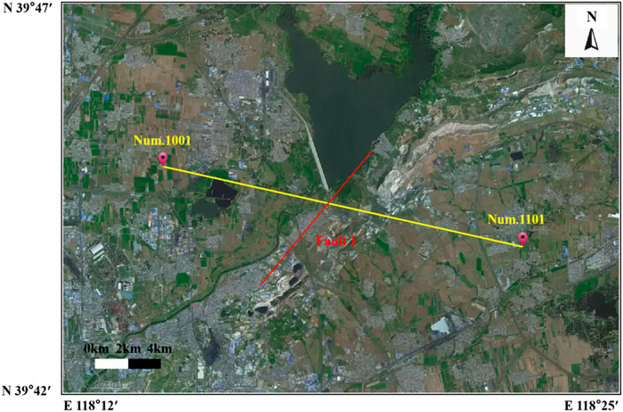
Figure 1. Distribution of station map.

3.2 Single station data progressing

We picked the three-component waveform of 1 day and calculated his power spectrum, where the waveform is shown in Figure 2 and the power spectrum is shown in Figure 3. We can see that the original ambient noise is smoother, which is favorable for subsequent cross-correlation calculation and dispersion curve extraction. Through the power spectrum, we can know that the ambient - noise - related energy is mainly concentrated in the following 15 Hz, in which there is an obvious horizontal energy axis in 2–5 Hz, indicating that there is a strong surface wave energy in this frequency range, which provides a reference band for the selection of the frequency band of the later cross-correlation calculation.

Figure 2

Figure 2. Raw ambient noise data waveform.

Figure 3

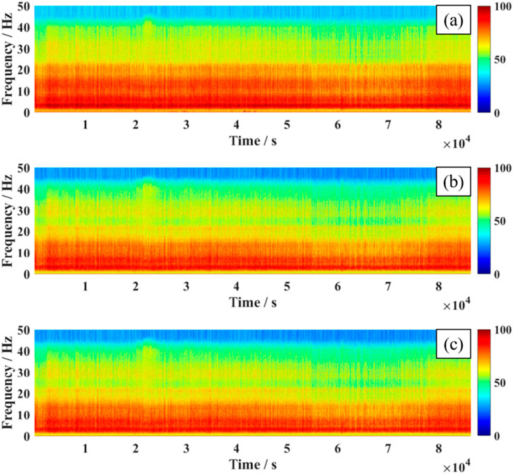
Figure 3. Power spectral density image. (a-c) show the power spectral density of the three-component ambient noise waveform (East [E], North [N], and Vertical [Z] components, respectively).

3.3 Ambient noise cross - Correlation analysis

Data preprocessing followed the processing flow of Bensen et al. (2007). First, the data quality of the continuous waveform from a single station is checked and bad channels are removed, the vertical component waveform is cut into 1-day data segments, the data segments are de-meaned and de-trended, the time-domain normalized, and the frequency-domain spectral whitened, respectively, and the original 100 Hz sampled data is re-sampled to 20 Hz to improve the computational velocity and band-pass filtered from 0.14 s to 10 s. The data undergo processing to enhance the signal-to-noise ratio. Finally, all stations are combined two by two to calculate the cross-correlation and stack the cross-correlation results to improve the signal-to-noise ratio (SNR). Finally, 5050 cross - correlation functions were computed from seismic ambient noise data of 101 stations. As depicted in Figure 4, cross - correlation functions for all station pairs of 1001 stations (totaling 100 entries) are presented. Here, (a)–(f) represent stacked cross - correlation profiles with frequency bands 0.14–10 s, 0.14–1 s, 1–3 s, 3–5 s, 5–10 s, and 3–10 s, respectively. Acquired signals exhibit a high SNR; however, signals on positive and negative half-axes are not fully symmetric, with positive half - branch signals notably stronger than negative ones. This asymmetry mainly stems from uneven noise source distribution.

Figure 4

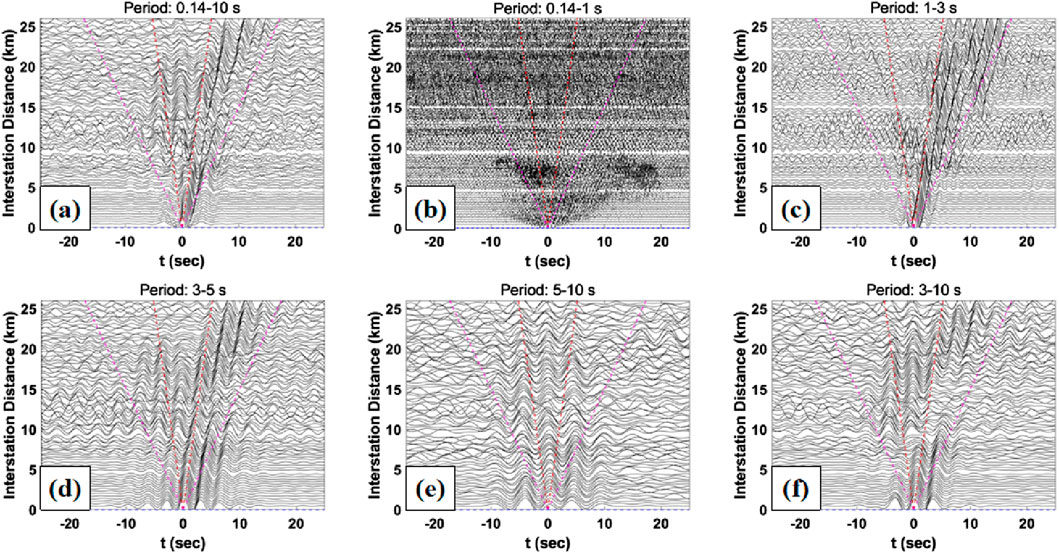
Figure 4. Cross-correlation stack profiles for different periods, where (a–f) are the cross-correlation stack profiles for 0.14–10s, 0.14–1s, 1–3, 3–5s, 5–10s, 3–10s, respectively.

3.4 Dispersion curse measurement

The empirical Green’s function can be derived by applying the Hilbert transform to cross-correlation functions. In this work, we employ the phase shift method on cross-correlation functions to generate dispersion energy diagrams and measure Rayleigh wave phase velocity phase velocity measurement s. As standard practice, stacking and averaging the positive and negative branches helps reduce artifacts caused by uneven noise source distributions. However, as the positive and negative branches in a linear array’s cross-correlation characterize noise sources originating from opposite ends of the array, this work employs three distinct dispersion energy calculation strategies to prevent possible cancellation of valid signals during averaging: utilizing the positive branch data alone, utilizing the negative branch data alone, and stacking both branches. This approach provides multiple alternatives for dispersion curve extraction.

When calculating the dispersive energy, the aperture of the sub-station array is set to 2 km, and the scanning frequency band is 0.3Hz–2 Hz; in Figure 5 the dispersive energy map of the phase-shift method, we can see that the dispersive energy distributions of the positive branch, the negative branch, and the positive and negative stack of the two branches are not uniform, in which the energy of the negative branch has more low-frequency energy, which is mainly concentrated in the range of 0.13–0.7 Hz, and that the energy of the positive branch has more high-frequency energy, which is mainly concentrated in the range of 0.2–0.85 Hz range. The stack of the positive and negative branches can significantly broaden the frequency range, mainly concentrated in the range of 0.13–0.85 Hz. However, the part less than 0.2 Hz shows obvious convex and concave, whether this part of the energy can be extracted and inverted needs to be considered from the overall distribution of the dispersion curve, and can not be singled out.

Figure 5

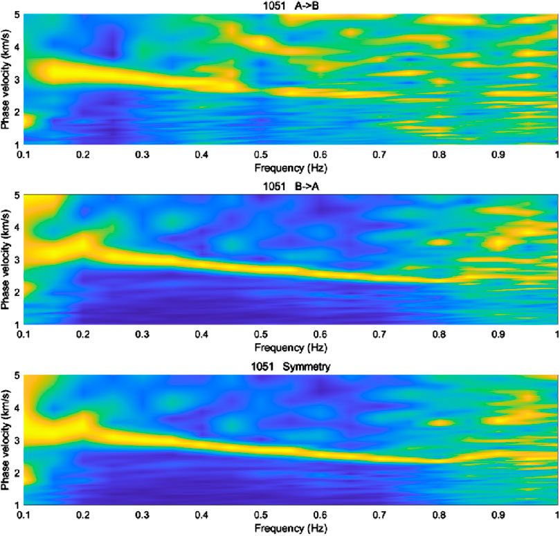B," shows a gradual color transition from blue to yellow across frequencies. The middle map, "B->A," exhibits similar patterns but with slight variations. The bottom map, labeled "Symmetry," maintains a consistent gradient, indicating symmetry between the two conditions." id="F5" loading="lazy">

Figure 5. Dispersion energy map for Station Num. 1051.

Through beamforming with the dense array, 101 dispersion curves were obtained. Figure 6 displays the dispersion curve distribution and the average dispersion curve, where the red solid line denotes the mean dispersion curve and the black solid line indicates the positive/negative standard deviation. The phase velocity of the mean dispersion curves spans 2.1–3.1 km/s, with periods ranging from 0.5 to 3 s.

Figure 6

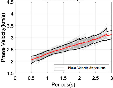
Figure 6. Distribution of dispersion curves, where the red solid line represents the average dispersion curve and the black line represents the positive and negative standard deviations.

4 Phase velocity tomography

4.1 Method

4.1.1 Parameterization

As described in Zhang et al. (2018), our subsurface modeling approach utilizes Voronoi tessellation for parameterization. Each Voronoi cell consists of a central site (reference point) and its corresponding spatial domain, containing all locations that are nearer to this site than to any other. Figure 7 demonstrates examples of Voronoi partitioning in one-, two-, and three-dimensional spaces, with each cell storing both spatial coordinates and physical parameters including P-wave velocity, S-wave velocity, and density. It should be noted that 1D Voronoi parameterization shows inferior performance compared to conventional zonal modeling approaches, since different cell arrangements may produce identical velocity structures. Considering that seismic surface waves are mainly sensitive to subsurface S-wave velocity variations, our inversion procedure concentrates exclusively on determining shear-wave velocity distributions. P - wave velocities are linked to shear - wave velocities via an empirical relationship:

$\text{Vp}=1.16\text{Vs}+1.36$

Figure 7

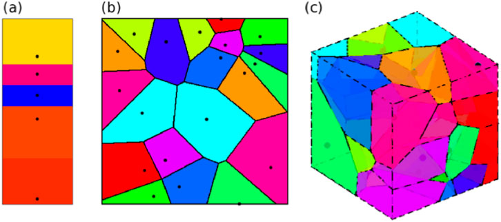
Figure 7. (a) Example of 1D Voronoi delineation, (b) Example of 2D Voronoi delineation, and (c) Example of 3D Voronoi delineation of velocity model. The colors represent the seismic velocities in each cell. The black dots represent the locations where each cell is generated.

The density was calculated from empirical values of P-wave velocity:

$\mathrm{\rho }=1.74\text{Vp}$

Vp and Vs. are in km/s, and density ρ is in g/cm³. Analogous to Zhang et al. (2018) velocity remains spatially uniform within each Voronoi cell.

4.1.2 2-Step inversion

First, through tomographic inversion using source-receiver arrival time data, we obtain 2D phase and group velocity maps at multiple frequencies. Then, for every geographical point, we perform 1D inversion of the shear-wave velocity profile using its local dispersion curve.

In the second step, a linear inversion approach (Galetti et al., 2017; Young et al., 2013) is employed to solve for the 1D shear velocity profile at each point. Conventionally, these 1D depth inversions are executed independently at each geographic site without inter-site interaction, a strategy that enables perfect parallelization of this computationally intensive task.

4.1.3 Fully 3D inversion

To construct a three-dimensional Vs. model and facilitate comparative analysis of inversion outcomes obtained through distinct methodologies, we performed parallel 3D inversions employing the Markov Chain Monte Carlo (MCMC) technique established in Zhang et al. (2018). The subsurface domain was discretized using Voronoi tessellation (Figure 7c), where each polyhedral cell is defined by its spatial position and Vs. value. Consistent with Zhang et al. (2018), the orthorectification procedure implements a dual-stage approximation process (Ritzwoller and Levshin, 1998; Stevens et al., 2001; Reiter and Rodi, 2008): Initial phase/group velocity maps are produced for individual periods by deriving Vs. profiles beneath surface points and implementing Herrmann’s (Herrmann, 2013) one-dimensional modal approximation to compute associated phase and group velocities; For each Voronoi model we discretize the subsurface into 50 m vertical layers down to 5 km depth, keeping the Vs. value of each Voronoi cell constant within its polyhedron. Phase velocities are computed at 0.05 s intervals over the 0.5–3 s period band using the fast-delta matrix algorithm. The dispersion integral uses a 1-D mode summation with 5 points per minimum wavelength and a 0.5% frequency-domain smoothing kernel to suppress numerical ringing. Ray tracing for travel-time calculation adopts a 2-D linear interpolation on the generated phase-velocity maps with a 20 m grid spacing, ensuring accurate path integration for the 120 m station spacing. Subsequent travel time determinations are made via ray tracing through the generated phase velocity maps for all source-receiver and inter-receiver paths.

To ensure the modal approximation software package was appropriate for our inversion, we imposed an a priori constraint requiring the minimum shear-wave velocity to occur at the surface. This constraint is enforced in the Markov chain by applying substantial penalties and rejecting any proposals violating this condition. Since this requirement generally holds true for most real Earth scenarios, we consider this both a geophysically valid and computationally feasible solution.

4.1.4 Reversible jump McMC

MCMC refers to a category of sampling algorithms that generate sequential samples (or chains) from specified probability distributions (Sivia, 1996). In this study, we implement an extended Metropolis-Hastings algorithm known as reversible jump MCMC (Green, 1995; Green and Hastie, 2009). This approach enables trans-dimensional inversion, meaning the number of model parameters may vary during the sampling process. As a result, the seismic velocity model’s parameterization can be determined directly from the data and prior knowledge, removing the need to predefine the parameterization before inversion (Galetti et al., 2017; Young et al., 2013; Zhang et al., 2018). It should be noted that the specific selection of parameterization might impose constraints on the model and impact the final results (Hawkins et al., 2019).

In seismic tomography applications, the objective probability distribution is mathematically represented by the Bayesian posterior probability density function (pdf) for velocity model m given observed dataset d, denoted as p (m|d). As per Bayes’ theorem:

$\mathit{p}\left(\mathit{m}|{\mathit{d}}_{\mathit{obs}}\right)=\frac{\mathit{p}\left({\mathit{d}}_{\mathit{obs}}\left.\right|\mathit{m}\right)\mathit{p}\left(\mathit{m}\right)}{\mathit{p}\left({\mathit{d}}_{\mathit{obs}}\right)}$

The conditional probability p (d_obs|m), termed the likelihood function, quantifies the probability of obtaining the observed measurements assuming model m is correct. The prior distribution p(m) encapsulates existing knowledge about model parameters independent of observational data d, whereas p (d_obs) functions as a normalizing constant referred to as the marginal likelihood. Our implementation adopts a Gaussian error model for the likelihood function, where data variance is incorporated as an auxiliary parameter and estimated through hierarchical inversion. For the prior probability density function, we use a non-informative prior with uniform distributions over wide bounds for each parameter. In the reversible jump Metropolis-Coupling algorithm, a new model m' is sampled from a proposal distribution q (m’|m) that depends on the current model m. The probability of accepting or rejecting this distribution, α(m’|m), is known as the acceptance rate, given by Green (1995):

$\mathit{\alpha }\left({\mathit{m}}^{\prime }|\mathit{m}\right)=\mathit{min}\left[\mathrm{1},\frac{\mathit{p}\left({\mathit{m}}^{\prime }\right)}{\mathit{p}\left(\mathit{m}\right)}\times \frac{\mathit{q}\left(\mathit{m}|{\mathit{m}}^{\prime }\right)}{\mathit{q}\left({\mathit{m}}^{\prime }|\mathit{m}\right)}\times \frac{\mathit{p}\left({\mathit{d}}_{\mathit{obs}}|{\mathit{m}}^{\prime }\right)}{\mathit{p}\left({\mathit{d}}_{\mathit{obs}}|\mathit{m}\right)}\times \left|\mathit{J}\right|\right]$

The Jacobian matrix J, facilitating the transformation between parameter spaces m and m', is employed to compute volumetric changes during trans-dimensional jumps. In our implementation, the Jacobian matrix can be mathematically demonstrated to be unitary.The model acceptance procedure involves: Generating a uniformly distributed random number within [0,1], comparing this value with the acceptance probability α, accepting the proposed model if the random number is less than α, retaining the current model as the subsequent sample if rejected. This acceptance mechanism, through careful design of α, ensures the Markov chain’s stationary distribution converges to the target Bayesian posterior p (m|d) given adequate sampling (Green, 1995).

For fixed-dimensional perturbations (cell movements, velocity changes, and data noise hyperparameter adjustments), we employ Gaussian proposal distributions (Zhang et al., 2018). For trans-dimensional perturbations (adding or removing cells), we opt to use the prior probability density function as the proposal distribution, as this approach yields higher acceptance rates compared to Gaussian distributions (Zhang et al., 2018; Dosso et al., 2014).

4.2 Data progressing application on north China

4.2.1 Sensitive kernel

Given the strong sensitivity of Rayleigh wave phase velocity to S-wave velocity structure within depths of approximately 1/3 wavelength (Xu et al., 2007), we derived a 1D average S-wave velocity model from the phase velocity dispersion data. For each period, the average S-wave velocity at its corresponding depth served as the starting model (Xia et al., 1999). Figure 8 displays the depth sensitivity kernels for fundamental-mode Rayleigh wave phase velocities across periods of 1.0–5.0 s. The results demonstrate that phase velocity sensitivity depth progressively increases with longer periods. Specifically, 1 s, 2 s, and 3 s period Rayleigh wave phase velocities offer superior constraints for shallow subsurface structures above 4 km depth. For structures deeper than 4 km, the discriminatory power of Rayleigh phase velocities decreases for all periods, but the data with a period of 5 s still exhibit a certain degree of sensitivity at 5 km depth. This indicates that the phase velocity dispersion curves extracted in this study can roughly invert the S-wave velocities at a depth of up to 5 km along the near-surface survey line.

Figure 8

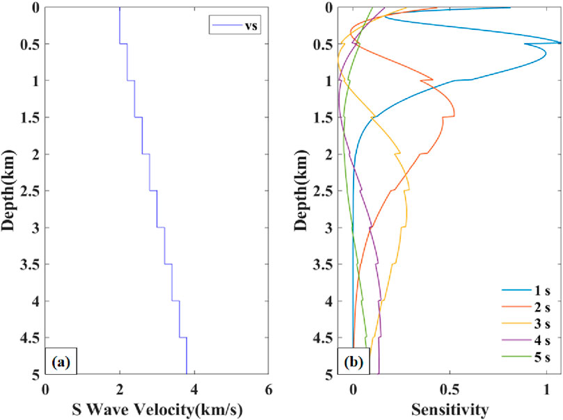
Figure 8. One-dimensional S-wave velocity model and phase velocity-sensitive kernels with different periods, (a) one-dimensional average S-wave velocity initial reference model, (b) sensitive kernels with phase velocities of different periods.

4.2.2 1D MCInversion

The S-wave velocity structure is determined by applying the previously described methodology to the obtained dispersion data, followed by comparative analysis of the results. Here, we invert for the Vs. structure utilizing fundamental-mode Rayleigh wave phase velocity dispersion data. 101 dispersion curves are extracted. 1D MC inversion is faster compared to 3D MC inversion. We extracted 101 dispersion curves. The 1D MC inversion is faster compared to the 3D MC inversion, and we performed 100,000 inversions using the 1D and 3D methods, respectively, to obtain the final results. Since the whole array is linear, we set the grid in the north direction as a thin plate during the 3D inversion, and then averaged all the results to get our results. 1D inversion is obviously not so cumbersome, and we can just follow the single-point inversion.

For the 1D MC depth inversion, the prior pdf for layer number was selected as a discrete uniform distribution (2–20 layers), with shear velocity prior set to 1500–4000 m/s. In 3D rj-MCMC steps (births/deaths), widths were chosen to maximize acceptance rate. For each geographic location, four chains ran for 100,000 iterations, with the first 50,000 as warm-up (samples ignored for inference). Every 100 samples post-warm-up were retained to estimate posterior pdf mean and standard deviation. The 3D inversion used a cell number prior of discrete uniform (400–1500), same as 1D, with noise hyperparameter priors uniformly distributed (0.0001–0.02 and 0.0–0.1). Trans-dimensional steps employed the prior as the proposal distribution.

For the 1D inversion, the inversion results for a single station are shown in Figure 9, where (a) (b) (c) (d) are the RMSE, confidence, likelihood function and S-velocity inversion results for a single station, respectively. We can see that the number of inversions has stabilized after 200 times, and from the likelihood function, the number of inversions is 400, which produces a fluctuation, and then quickly stabilizes. The fitting of the observed data obtained from the inversion to the modeled data and the distribution of the PDF are shown in Figure 10, and we can see that the observed data and the modeled data have been close, but not exactly the same. The confidence level of the overall model is high, between 0.80 and 1.0.

Figure 9

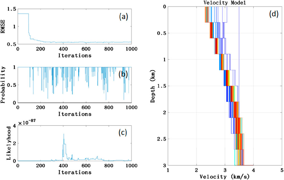
Figure 9. 1D MC single station inversion results, (a–d) are the RMSE, confidence, likelihood function and S-wave velocity inversion results for a single station respectively.

Figure 10

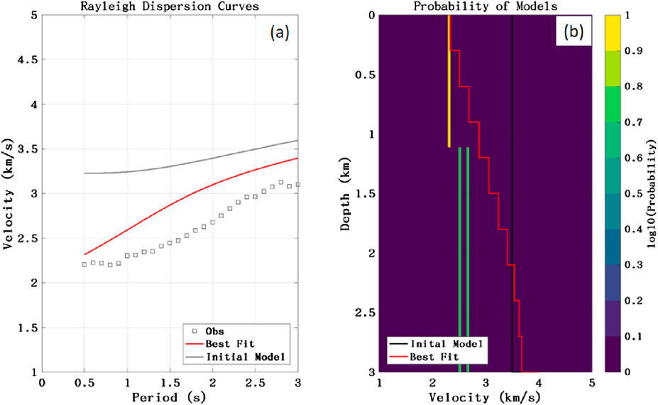
Figure 10. 1D MC single station inversion PDF distribution, (a) shows the comparison of dispersion curves before and after inversion, (b) shows the posterior probability density distribution after inversion.

After inverting all the dispersion curves through the same steps mentioned above, we arrange all the S-wave velocities according to their relative positions, and finally get the S-wave velocity profile of the whole station array, see Figure 11. We can see that the overall velocity range is distributed between 2.0–4.0 km/s, which has a relatively complete structure, but due to the lack of S-regularization, the final result does not bring out the structure very well.

Figure 11

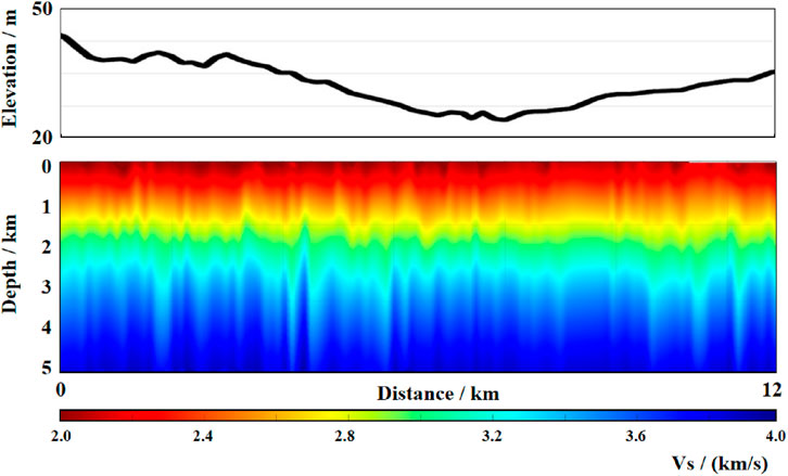
Figure 11. 1D MC S wave inversion profile.

For 3D rj-MCMC we follow the above steps to invert the profile, and finally obtain the S-wave velocity mean profile (see Figure 12) and standard deviation profile (see Figure 13) for the whole profile. The profile after 3D rj-MCMC inversion has stronger continuity, and the overall trend is concave in the middle. The standard deviation profile shows a more obvious depression from 2 km depth to 5 km depth, with a clear blue band at 1 km depth, a clear break from 6 km to 10 km horizontally, and a reappearance of the previous blue band from 10 km to 12 km The depth from 0 to 5 km is divided into three main layers, which are 0–1 km, 1–3 km, 3–5 km (Interpreted structures: 0–1 km, Vs. = 2.10 ± 0.05 km/s; 1–3 km, Vs. = 2.75 ± 0.08 km/s; 3–5 km beneath the F1 trace, Vs. = 2.95 ± 0.12 km/s), respectively, three main tomography layers.

Figure 12

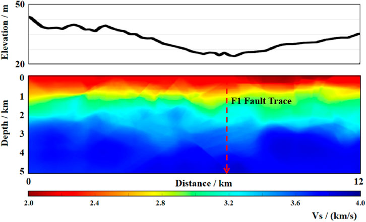
Figure 12. 3D rj-MCMC inversion S-wave velocity mean profile. Red dashed line marks the surface trace of the F1 fault (x = 6–10 km); red arrow indicates its inferred extension to 5 km depth inferred from the velocity discontinuity.

Figure 13

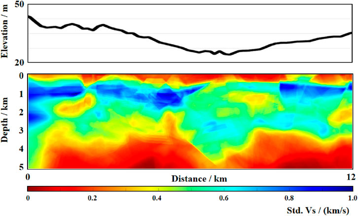
Figure 13. 3D rj-MCMC inversion S-wave velocity standard deviation profile.

The model domain extends 0–12 km horizontally and 0–5 km vertically. Voronoi cells parameterise the model, with the number of cells drawn from a discrete uniform prior Ncell ∼ U (400, 1 500). Each cell is assigned an S-wave velocity Vs. ∼ U (1.5, 4.0) km s^-1; Vp and ρ follow Vp = 1.16V s. + 1.36 km s^-1 and ρ = 1.74 Vp g cm^-3. Two noise hyper-parameters are used: data-error σ₁ ∼ U (0.0001, 0.02) and model-error σ₂ ∼ U (0.0, 0.1). Four parallel Markov chains were run for 100,000 iterations; the first 50,000 were discarded as burn-in, and every 100th sample thereafter was retained, yielding 500 posterior models. Fixed-dimensional moves employ Gaussian proposals tuned during pilot runs; trans-dimensional steps use the prior as the proposal distribution, yielding acceptance rates of ≈23% and ≈18%, respectively.

4.3 Model uncertainty quantification

We define “model uncertainty” as one standard deviation (1σ) of the posterior probability density function (PDF), obtained in three steps:

1. Posterior sampling: for every 3-D rj-MCMC chain, we retain one model every 100 iterations from iterations 50,001–100 000 after burn-in, yielding 500 retained models;

2. Voxelization: each of the 500 Voronoi models is resampled onto a regular grid with 20 m × 20 m × 20 m voxels, giving an ensemble of Vs. values {Vs._i} for every voxel;

3. Statistics: the mean μ and standard deviation σ of {Vs._i} are computed for each voxel—μ is taken as the “best” model, and σ is taken as the model uncertainty.

To examine how data constraint strength influences σ, we simultaneously calculate the data kernel density (DK), defined as the number of ray paths traversing a voxel divided by the voxel volume. Regions where DK < 10 ray paths/km³ are masked in gray in Figure 13, alerting readers that the elevated uncertainty there is primarily due to data sparsity rather than algorithmic limitations.

4.4 Synthetic resolution and checkerboard validation

To quantify the spatial resolution improvement of the fully 3-D inversion over the traditional 1-D approach, we conducted checkerboard and point-anomaly tests. A synthetic model consisting of alternating ±10% Vs. anomalies (1 km × 1 km × 0.5 km blocks) was embedded in a 1-D background profile and forward-modelled to dispersion curves (0.5–3 s) with the same noise level as the observed data. The 3-D transdimensional inversion recovered >80% of the anomaly amplitude in the upper 3 km and correctly delineated block boundaries within ±100 m, whereas the 1-D inversion exhibited vertical smearing and recovered only ∼40% amplitude. A point-anomaly test (200 m × 200 m × 200 m) showed that lateral resolution of the 3-D scheme reaches ∼2/3 wavelength (≈400 m at 1 s), corresponding to a ∼40% improvement in locating sharp velocity contrasts compared with the 1-D scheme. These tests confirm that the 3-D Bayesian framework delivers the resolution gain claimed in the manuscript.

5 Discussion

The three-dimensional Bayesian Monte Carlo inversion results delineate the shear-wave velocity (Vs.) structure in the uppermost 5 km beneath the northeastern boundary region of the North China Craton (NCC). Compared with traditional 1D independent inversions, the 3D results (Figure 12) exhibit a prominent lateral velocity gradient zone at 6–10 km horizontal position, whose spatial orientation aligns with the strike of the F1 fault crossed by the survey line. This velocity discontinuity likely corresponds to lithospheric shear zones formed during the NCC destruction process (Zhu et al., 2012). The standard deviation profile (Figure 13) reveals a distinct low-velocity anomaly (2.8–3.1 km/s) beneath the fault at 3–5 km depth, spatially consistent with the Cenozoic basalt conduit model in the eastern NCC. To evaluate whether the low-velocity anomaly beneath the F1 fault is statistically significant, we performed a two-tailed Bayesian credibility test on the voxel-wise posterior Vs. distribution. Within the anomalous zone (x = 6–10 km, z = 3–5 km), 94.7% of the posterior Vs. samples fall below the median Vs. of the surrounding high-velocity wall-rock (3.35 km s^-1), yielding a 94.7% posterior probability (equivalent to p < 0.053 in frequentist terms) that the anomaly is genuine. A bootstrap Kolmogorov–Smirnov test (1 000 resamples) further rejects the null hypothesis that the Vs. distributions inside and outside the anomaly come from the same population (D = 0.29, p < 0.01). These results confirm that the fault-related low-velocity anomaly is statistically significant at the 95% confidence level. This suggests that the Late Mesozoic cratonic destruction events may have left structural imprints of deep melt infiltration.

The high-velocity layer at 0–1 km depth correlates well with the widely exposed Archean basement rocks in the NCC (Zh et al., 2005). The interlayer (2.6–2.9 km/s) at 1–3 km depth revealed by 3D inversion may represent sedimentary basin structures formed during the Mesozoic intracontinental rifting stage, showing spatiotemporal consistency with the Late Jurassic fault-depression sequences identified in regional seismic surveys. Notably, our transdimensional inversion strategy effectively mitigates velocity ambiguity artifacts caused by traditional two-step methods in cratonic complex tectonic zones (Zhang et al., 2018), providing a novel technical approach for resolving multiphase tectonic superposition in NCC destruction areas.

To quantify the reliability of our 3-D Vs. model, we conducted three complementary tests. A checkerboard resolution experiment (±10%, 1 km blocks) achieved >80% recovery down to 3 km but only ∼55% at 4–5 km, validating the σ-based uncertainty pattern in Figure 13. Bootstrap resampling of 100 random 80 %-station-pair subsets yielded inter-quartile Vs. ranges within 5% of the MCMC 1 σ posterior interval, confirming the consistency of the derived σ. Finally, an exponential relationship between σ and data-kernel density (σ ≈ 0.14 e^(-0.06 DK), R² = 0.71) shows that the elevated σ at 4–5 km is dominated by data sparsity rather than inversion bias.

In summary, Bayesian inversion in two-step approaches may cause data overfitting and biased results. However, noise estimation is often challenging, and improper noise levels can degrade model resolution. This issue can be partly mitigated by incorporating additional data (e.g., higher-mode dispersion curves). Alternatively, our results show that using 3D parameterization with S-spatial correlations in inversion effectively addresses this problem.

This study compares two methods for estimating shear-wave velocity models using only fundamental-mode data. Future work will involve 3D inversion with higher-order dispersion data to better constrain subsurface structures and enhance deep-resolution capabilities.

Regarding computational costs, a single 3D inversion chain requires approximately 312.3 CPU hours, while 1D MC inversion consumes only 27.4 CPU hours per chain. Notably, 3D rj-MCMC inversion yields a significantly more detailed 3D S-wave velocity structure, justifying the higher computational investment in terms of cost-effectiveness.

6 Conclusion

This study pioneers the application of 3D Bayesian Monte Carlo inversion to near-surface structural imaging in the North China Craton (NCC) destruction belt. Comparative analyses reveal three key findings: 1) The 3D-derived S-wave velocity model improves lateral resolution by ∼40%, clearly delineating velocity contrasts (ΔVs = 0.3–0.5 km/s) within 2 km across the F1 fault zone. This correlates with the brittle-ductile transition depth (∼5 km) of reactivated cratonic margin faults. 2) Uncertainty analysis shows higher velocity standard deviations (σ = 0.12–0.15 km/s) at 3–5 km depth within the destruction zone compared to stable cratonic cores (σ < 0.08 km/s), reflecting enhanced lithospheric heterogeneity caused by destruction processes. 3) The high-resolution velocity model provides near-surface evidence for Mesozoic tectonic transition events in the eastern NCC (Zhu and Xu, 2019). Future integration with deep seismic anisotropy data could unravel crust-mantle coupling mechanisms during cratonic destruction.

Data availability statement

The original contributions presented in the study are included in the article/supplementary material, further inquiries can be directed to the corresponding author.

Author contributions

YL: Data curation, Investigation, Project administration, Conceptualization, Methodology, Formal Analysis, Writing – review and editing, Writing – original draft. BW: Methodology, Investigation, Conceptualization, Writing – review and editing. DY: Writing – original draft, Validation, Project administration, Methodology. LZ: Investigation, Conceptualization, Writing – review and editing. JW: Methodology, Conceptualization, Project administration, Writing – original draft, Investigation. TZ: Validation, Methodology, Writing – review and editing.

Funding

The author(s) declare that financial support was received for the research and/or publication of this article. This study is funded by the Science and Technology Development Plan Project of Jilin Province, China Grant (Grant No. 20210101107JC) and Science and Technology Research Project of Jilin Provincial Department of Education (Grant No. JJKH20200267KJ).

Conflict of interest

The authors declare that the research was conducted in the absence of any commercial or financial relationships that could be construed as a potential conflict of interest.

Generative AI statement

The author(s) declare that no Generative AI was used in the creation of this manuscript.

Any alternative text (alt text) provided alongside figures in this article has been generated by Frontiers with the support of artificial intelligence and reasonable efforts have been made to ensure accuracy, including review by the authors wherever possible. If you identify any issues, please contact us.

Publisher’s note

All claims expressed in this article are solely those of the authors and do not necessarily represent those of their affiliated organizations, or those of the publisher, the editors and the reviewers. Any product that may be evaluated in this article, or claim that may be made by its manufacturer, is not guaranteed or endorsed by the publisher.

References

Aki, K., and Richards, P. G. (1980). Quantitative seismology.

Google Scholar

Allmark, C., Curtis, A., Galetti, E., and de Ridder, S. (2018). Seismic attenuation from ambient noise across the north sea ekofisk permanent array. J. Geophys. Res. Solid Earth 123, 8691–8710. doi:10.1029/2017jb015419

CrossRef Full Text | Google Scholar

Bensen, G. D., Ritzwoller, M. H., Barmin, M. P., Levshin, A. L., Lin, F., Moschetti, M. P., et al. (2007). Processing seismic ambient noise data to obtain reliable broad-band surface wave dispersion measurements. Geophys. J. Int. 169 (3), 1239–1260. doi:10.1111/j.1365-246x.2007.03374.x

CrossRef Full Text | Google Scholar

Burdick, S., and Lekić, V. (2017). Velocity variations and uncertainty from transdimensional p-wave tomography of North America. Geophys. J. Int. 209 (2), 1337–1351. doi:10.1093/gji/ggx091

CrossRef Full Text | Google Scholar

Curtis, A., Trampert, J., Snieder, R., and Dost, B. (1998). Eurasian fundamental mode surface wave phase velocities and their relationship with tectonic structures. J. Geophys. Res. 103 (B11), 26919–26947. doi:10.1029/98jb00903

CrossRef Full Text | Google Scholar

Dosso, S. E., Dettmer, J., Steininger, G., and Holland, C. W. (2014). Efficient trans-dimensional Bayesian inversion for geoacoustic profile estimation. Inverse Probl. 30 (11), 114018. doi:10.1088/0266-5611/30/11/114018

CrossRef Full Text | Google Scholar

Galetti, E., and Curtis, A. (2018). Transdimensional electrical resistivity tomography. J. Geophys. Res. Solid Earth 123, 6347–6377. doi:10.1029/2017jb015418

CrossRef Full Text | Google Scholar

Galetti, E., Curtis, A., Meles, G. A., and Baptie, B. (2015). Uncertainty loops in travel-time tomography from nonlinear wave physics. Phys. Rev. Lett. 114 (14), 148501. doi:10.1103/physrevlett.114.148501

PubMed Abstract | CrossRef Full Text | Google Scholar

Galetti, E., Curtis, A., Baptie, B., Jenkins, D., and Nicolson, H. (2017). Transdimensional Love-wave tomography of the British isles and shear-velocity structure of the east Irish sea basin from ambient-noise interferometry. Geophys. J. Int. 208 (1), 36–58. doi:10.1093/gji/ggw286

CrossRef Full Text | Google Scholar

Green, P. J. (1995). Reversible jump markov chain monte carlo computation and Bayesian model determination. Biometrika 82, 711–732. doi:10.1093/biomet/82.4.711

CrossRef Full Text | Google Scholar

Green, P. J., and Hastie, D. I. (2009). Reversible jump MCMC. Genetics 155 (3), 1391–1403.

Google Scholar

Han, C., Liang, F., Li, H. L., Wang, T., Zhang, M., and Tang, L. (2022). Research on the application of auto-correlation and HVSR joint imaging based on ambient noise in the detection of urban shallow structures in huizhou. Geol. Rev. 68 (04), 1413–1422. doi:10.16509/j.georeview.2022.06.151

CrossRef Full Text | Google Scholar

Hastings, W. K. (1970). Monte carlo sampling methods using markov chains and their applications. Biometrika 57 (1), 97–109. doi:10.2307/2334940

CrossRef Full Text | Google Scholar

Hawkins, R., and Sambridge, M. (2015). Geophysical imaging using trans-dimensional trees. Geophys. J. Int. 203 (2), 972–1000. doi:10.1093/gji/ggv326

CrossRef Full Text | Google Scholar

Hawkins, R., Bodin, T., Sambridge, M., Choblet, G., and Husson, L. (2019). Trans-dimensional surface reconstruction with different classes of parameterization. Geochem. Geophys. Geosystems 20 (1), 505–529. doi:10.1029/2018gc008022

CrossRef Full Text | Google Scholar

Herrmann, R. B. (2013). Computer programs in seismology: an evolving tool for instruction and research. Seismol. Res. Lett. 84 (6), 1081–1088. doi:10.1785/0220110096

CrossRef Full Text | Google Scholar

Luo, K., Zong, Z., Yin, X., Zuo, Y., Fu, Y., and Zhan, W. (2025). Shale pore pressure seismic prediction based on the hydrogen generation and compaction-based rock-physics model and bayesian hamiltonian monte carlo inversion method. GEOPHYSICS 90 (2), M15–M30. doi:10.1190/geo2024-0325.1

CrossRef Full Text | Google Scholar

Malinverno, A. (2002). Parsimonious bayesian markov chain monte carlo inversion in a nonlinear geophysical problem. Geophys. J. Int. 151 (3), 675–688. doi:10.1046/j.1365-246x.2002.01847.x

CrossRef Full Text | Google Scholar

Malinverno, A., and Briggs, V. A. (2004). Expanded uncertainty quantification in inverse problems: hierarchical bayes and empirical bayes. Geophysics 69 (4), 1005–1016. doi:10.1190/1.1778243

CrossRef Full Text | Google Scholar

Malinverno, A., and Leaney, S. (2000). “A monte carlo method to quantify uncertainty in the inversion of zero-offset VSP data,” in Proceedings of the 2000 SEG annual meeting[C] (Tulsa, Oklahoma: Society of Exploration Geophysicists).

Google Scholar

Metropolis, N., and Ulam, S. (1949). The monte carlo method. J. Am. Stat. Assoc. 44 (247), 335–341. doi:10.1080/01621459.1949.10483310

PubMed Abstract | CrossRef Full Text | Google Scholar

Mosegaard, K., and Tarantola, A. (1995). Monte carlo sampling of solutions to inverse problems. J. Geophys. Res. 100 (B7), 12431–12447. doi:10.1029/94jb03097

CrossRef Full Text | Google Scholar

Piana, A. N., Giacomuzzi, G., and Malinverno, A. (2015). Local three-dimensional earthquake tomography by trans-dimensional monte carlo sampling. Geophys. J. Int. 201 (3), 1598–1617. doi:10.1093/gji/ggv084

CrossRef Full Text | Google Scholar

Reiter, D. T., and Rodi, W. L. (2008). A new regional 3-D velocity model for Asia from the joint inversion of p-wave travel times and surface-wave dispersion data. Lexington, MA: Weston Geophysical.

Google Scholar

Ritzwoller, M. H., and Levshin, A. L. (1998). Eurasian surface wave tomography: group velocities. J. Geophys. Res. 103 (B3), 4839–4878. doi:10.1029/97jb02622

CrossRef Full Text | Google Scholar

Shapiro, N., and Campillo, M. (2004). Emergence of broadband rayleigh waves from correlations of the ambient seismic noise. Geophys. Res. Lett. 31 (7), L07614. doi:10.1029/2004gl019491

CrossRef Full Text | Google Scholar

Sivia, D. (1996). Data analysis: a bayesian tutorial. Oxford: Oxford University Press.

Google Scholar

Stevens, J. L., Adams, D. A., and Baker, G. E. (2001). Improved surface wave detection and measurement using phase-matched filtering with a global one-degree dispersion model. San Diego, CA: Science Applications International Corp.

Google Scholar

Wapenaar, K. (2004). Retrieving the elastodynamic Green’s function of an arbitrary inhomogeneous medium by cross correlation. Phys. Rev. Lett. 93 (25), 254301. doi:10.1103/physrevlett.93.254301

PubMed Abstract | CrossRef Full Text | Google Scholar

Wapenaar, K., and Fokkema, J. (2006). Green's function representations for seismic interferometry. Geophysics 71 (4), SI33–SI46. doi:10.1190/1.2213955

CrossRef Full Text | Google Scholar

Xia, J. H., Miller, R. D., and Park, C. B. (1999). Estimation of near-surface shear-wave velocity by inversion of rayleigh waves. GEOPHYSICS 64 (3), 691–700. doi:10.1190/1.1444578

CrossRef Full Text | Google Scholar

Xu, G. M., Yao, H. J., Zhu, L. B., and Shen, Y. S. (2007). Shear wave velocity structure of the crust and upper mantle in Western China and its adjacent area. Chin. J. Geophys. in Chin. 50 (1), 193–208. doi:10.1002/cjg2.1025

CrossRef Full Text | Google Scholar

Young, M. K., Rawlinson, N., and Bodin, T. (2013). Transdimensional inversion of ambient seismic noise for 3D shear velocity structure of the Tasmanian crust. Geophysics 78 (3), WB49–WB62. doi:10.1190/geo2012-0356.1

CrossRef Full Text | Google Scholar

Zhao, G., Sun, M., Wilde, S. A., and Li, S. Z. (2005). Late Archean to Paleoproterozoic evolution of the north China craton. Gondwana Res. 8 (3), 247–258. doi:10.1016/j.precamres.2004.10.002

CrossRef Full Text | Google Scholar

Zhan, W., Chen, Y., Liu, Q., Li, J., Sacchi, M. D., Zhuang, M., et al. (2024). Simultaneous prediction of petrophysical properties and formation layered thickness from Acoustic logging data using a modular cascading residual neural network (MCARNN) with physical constraints. J. Appl. Geophys. 224, 105362. doi:10.1016/j.jappgeo.2024.105362

CrossRef Full Text | Google Scholar

Zhang, X., Curtis, A., Galetti, E., and de Ridder, S. (2018). 3-D monte carlo surface wave tomography. Geophys. J. Int. 215 (3), 1644–1658. doi:10.1093/gji/ggy362

CrossRef Full Text | Google Scholar

Zhu, R., and Xu, Y. (2019). The subduction of the west Pacific plate and the destruction of the north China Craton. Sci. China Earth Sci. 62 (8), 1340–1350. doi:10.1007/s11430-018-9356-y

CrossRef Full Text | Google Scholar

Zhu, R. X., Yang, J. H., and Wu, F. Y. (2012). Timing of destruction of the north China craton. Lithos 149, 51–60. doi:10.1016/j.lithos.2012.05.013

CrossRef Full Text | Google Scholar

Zulfakriza, Z., Saygin, E., Cummins, P., Widiyantoro, S., Nugraha, A. D., Lühr, B. G., et al. (2014). Upper crustal structure of Central java, Indonesia, from transdimensional seismic ambient noise tomography. Geophys. J. Int. 197 (1), 630–635. doi:10.1093/gji/ggu016

CrossRef Full Text | Google Scholar