Geological information-driven deep learning for lithology identification from well logs

Lithology identification is crucial for characterizing complex unconventional reservoirs, where thin interlayers significantly influence hydrocarbon accumulation. Although deep learning-based methods utilizing well logs have become prevalent, most approaches treat well logs as generic 1D time series, frequently neglecting the multi-scale geological information inherent in the data. This oversight limits their accuracy and generalizability, especially in geologically complex environments. To overcome this limitation, we propose a novel geology-driven deep learning framework. Our key contribution is the transformation of 1D well logs into 2D multi-scale feature maps through multiresolution wavelet decomposition, a process designed to explicitly represent geological features resembling sedimentary cycles. These feature maps are subsequently processed by a novel Geology-Guided Hybrid Network with channel-spatial attention, which integrates a 2D CNN to capture geological patterns and a Bidirectional long short-term memory to model sequential dependencies. Evaluated on field data from complex reservoirs, our method achieves an outstanding F1-score of up to 0.966, outperforming four established deep learning benchmarks. Importantly, the approach demonstrates improved accuracy in identifying thin layers and enhanced generalization across wells with differing lithological distributions, attaining an F1-score of 0.885 on a challenging test well exhibiting significant data drift. This study validates the robustness of our geology-informed approach and offers an effective framework for high-precision lithology identification.

1 Introduction

Lithology identification in well logging plays a vital role in hydrocarbon exploration, particularly in structurally complex areas (Chang et al., 2021; Saporetti et al., 2019; Wang et al., 2024). Accurate subsurface lithology characterization provides essential scientific foundations for reservoir evaluation and development planning, as lithology directly controls the rock’s mechanical properties, pore structure, and fluid flow behavior, which are critical for evaluating reservoir extraction dynamics and safety (Wang et al., 2025; Teng et al., 2025; Cao et al., 2025). Traditional lithology identification methods primarily rely on empirical analysis and cross-plots (Liu Y et al., 2021). While these approaches can yield reasonable interpretations in simple geological conditions, their accuracy and efficiency face significant challenges when dealing with complex geological structures or large-scale multi-well data.

To overcome these challenges, machine learning (ML) techniques have been widely applied in processing well log data and lithology identification, such as support vector machines (Kumar T et al., 2022), random forests (Dev and Eden, 2019; Ao et al., 2020), and k-nearest neighbor algorithms (Wang et al., 2018). However, these methods predominantly rely on shallow ML algorithms. With the advancement of deep learning (DL), methods based on deep neural networks, such as convolutional neural networks (CNNs) and recurrent neural networks (RNNs), have achieved remarkable progress in lithology identification. Due to their strong local feature extraction capabilities and sensitivity to sequential data, these approaches have become mainstream in lithology identification (Dos Santos et al., 2022; Jaikla et al., 2019; Park et al., 2022; Wang et al., 2023; Lin et al., 2020). These models have demonstrated remarkable capabilities across various geological settings, leveraging the rich information contained within multi-type well logs to learn complex, non-linear relationships between log responses and lithological classes (Mukherjee B et al., 2024; Mohammadi K et al., 2025). The application of deep learning is increasingly focused on utilizing advanced deep learning models to address the ongoing challenge of characterizing thin layers, which typically have lower resolution than conventional methods (Ehsan M et al., 2024; Manzoor U et al., 2024).

Despite their successes, most DL methods treat well logs as simple one-dimensional time series, using 1D networks to extract depth-directional features while neglecting the rich geological and stratigraphic information embedded within. From a geological and sedimentological perspective, well log data reflect the physical and chemical properties of subsurface strata, which are directly linked to depositional environments, processes, and lithological characteristics (Song et al., 2021). Incorporating this geological context is crucial, as lithological variations are often influenced by stratigraphic sequences and depositional cycles (Li et al., 2024). Ignoring these factors may limit the predictive and generalization capabilities of ML and DL models in complex geological settings.

To address this limitation, previous studies have incorporated geological information in various ways. For example, Zhu et al. (2020) employed wavelet transform to divide well logs into multi-scale components and used a single 2-dimensional convolutional neural network (2DCNN) model for prediction. Jiang et al. (2021) integrated geological constraints into bidirectional gated recurrent units, while Sun et al. (2023) proposed a cross-domain lithology identification method combining wavelet transform and adversarial learning. Lv et al. (2024) introduced Gaussian windows to represent stratigraphic sequences with geological constraints, achieving notable results in identifying tight sandstone reservoirs. Pang et al. (2024) encoded raw well log data into graph structures using multi-dimensional spectral maps and applied spatio-temporal neural networks for lithology identification. Although these methods consider the geological information in well logs, they often fail to integrate geological features with temporal information, leading to challenges in accuracy and generalization in complex geological conditions.

This study proposes a novel geology-driven deep learning framework designed to explicitly incorporate multi-scale geological information into the identification process. The main contributions are as follows.

1. We propose a geology-informed feature engineering strategy based on multiresolution wavelet decomposition. This transforms conventional 1D well logs into 2D feature maps, where one axis represents depth and the other represents geological scale, making features analogous to sedimentary cycles explicitly available for model learning.

2. We design a novel hybrid deep learning architecture, the Geology-guided Channel-Spatial Attention Hybrid Network (CA-HybridNet). It synergistically combines a 2D ResNet to extract scale-dependent geological patterns, a Bidirectional LSTM to capture stratigraphic context, and a channel-spatial attention mechanism to focus on the most discriminative log types and depth intervals.

3. We validate our framework using field data from a complex reservoir in the Songliao Basin, demonstrating that our approach not only improves identification accuracy for challenging thin-bedded lithologies but also significantly enhances the model’s generalization and robustness.

2 Study area and data

The study area is located within the structural transition zone between the Sanzhao Depression and the Daqing Placanticline in the northern part of China’s Songliao Basin, specifically along the northwestern margin of the Sanzhao Depression adjacent to the Daqing Placanticline (Sun et al., 2007). This region, situated in the central depression zone of the northern Songliao Basin, exhibits gentle topographic dips of up to 0.2° and spans an area of approximately 100 km², as illustrated in Figure 1A. The target interval for this study is the Putaohua Member of the Yaojia Formation, which belongs to the Lower Cretaceous. Within one of the target intervals in the study area, three dominant sedimentary facies are developed: interdistributary bays, channels, and sheets sand. The well locations utilized are annotated in Figure 1B. Specifically, Well 1 and Well 2 were selected for testing, with Well 1 situated in the interdistributary facies and Well 2 positioned within the sand sheet facies. The target well-logging interval for model validation is primarily composed of four lithological types: shale, siltstone, sandstone, and calcareous sandstone. Their corresponding labels and sample distributions are presented in Table 1.

Figure 1

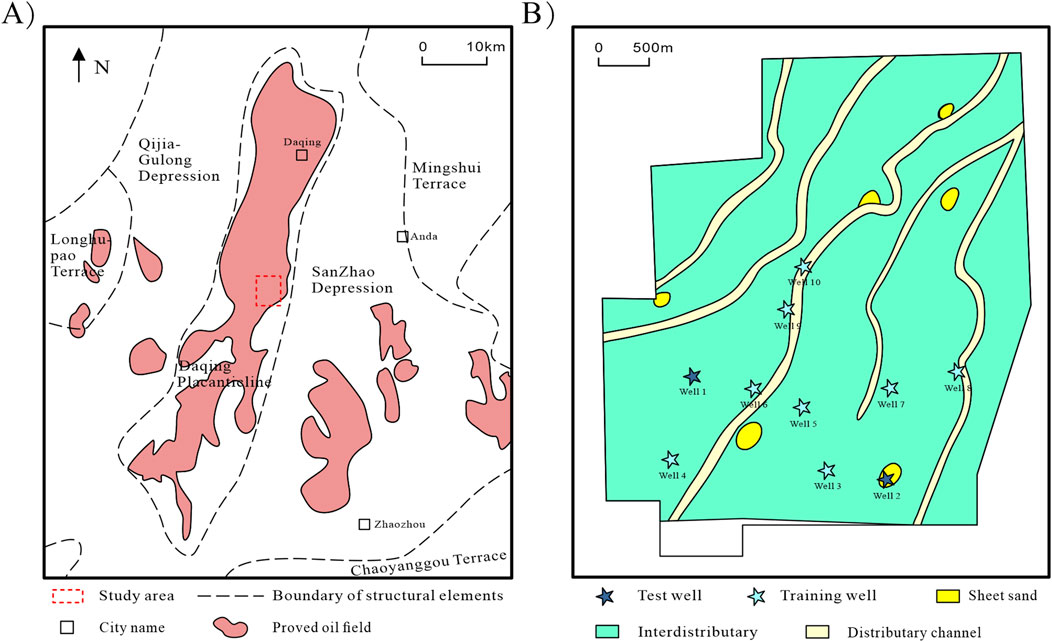
Figure 1. Geology and location of the wells. (A) Structural units division and study area location; (B) Sedimentary facies of the target interval and distribution of training/test wells in the study area (modified from Xu et al., 2023).

Table 1

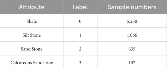
Table 1. Lithology attribute and samples.

In this study, well-logging data and lithological records from ten wells were utilized to evaluate the predictive performance of the proposed model. Based on the sensitivity relationships between lithologies and well log curves, we selected six curves for lithology identification (AC, GR, RLLD, RLLS, RMG, and RMN curves). The well log curve data were obtained from actual logging operations and digitized at a sampling interval of 0.125 m. Gamma ray (GR) logging, which measures natural radioactivity, plays a critical role in distinguishing between lithologies such as shale and non-shale formations (Wang et al., 2023). The acoustic (AC) curve provides information on formation porosity and lithology, aiding in the differentiation of various rock types. In addition, the deep laterolog resistivity (RLLD) and shallow laterolog resistivity (RLLS) curves are used together to assess formation resistivity at different depths, thereby enabling more accurate lithology interpretation. Furthermore, medium electrode spacing resistivity logging (RMG) and near electrode spacing resistivity logging (RMN) are combined to further refine lithology interpretation and enhance the ability to distinguish between different lithologies. Detailed information regarding the well log curves and lithologies can be found in Zhu et al., 2020 and will not be reiterated here. No seismic data were incorporated in the current work, demonstrating the potential of extracting rich geological information solely from well log measurements.

3 Methodology

The main workflow and neural network framework of this study are shown in Figure 2: First, multi-scale wavelet decomposition is applied to each well log curve, dividing it into components at different scales. The decomposed curves undergo normalization and other preprocessing steps. The processed data are then input into the proposed network model, where geological features are extracted by 2D convolution kernels, and temporal features are captured by the long short-term memory (LSTM) structure. The extracted features are flattened by a fully connected layer and finally passed through a Softmax function to output lithology identification results.

Figure 2

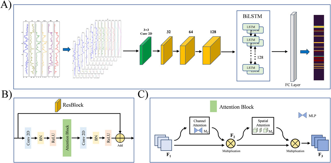
Figure 2. The framework of the proposed method for lithology identification (A). The network mainly includes a residual module (B), an attention module (C), and a BiLSTM module. Each logging curve is decomposed into multi-scale sub-curves through wavelet decomposition, which serves as the input data for the network, with the training target being the true logging lithology.

3.1 Multiresolution wavelet decomposition

In recent years, wavelet transform, as a multi-scale analysis tool, has been increasingly applied in well log data processing. By decomposing well logs into components across different frequency bands, hidden details in the data can be better revealed (Zhang et al., 2018). Unlike Fourier transform, wavelet transform provides simultaneous signal information in both the time and frequency domains. Therefore, in well log data processing, wavelet decomposition is particularly effective in capturing lithological variations.

From the perspective of high-resolution sequence stratigraphy, well log curves are not random series but are records of geological history, controlled by the cyclic rise and fall of the base level over different time scales. These base-level cycles, which can be categorized into long-term, mid-term, and short-term orders, govern the formation of depositional sequences and their internal stacking patterns (e.g., fining-upward or coarsening-upward trends). Multiresolution wavelet decomposition provides a powerful mathematical tool to deconstruct the well log signal into various frequency components that can be directly correlated with these different orders of geological cycles (Yu et al., 2023). The low-frequency components (smooth curves) capture the broad trends associated with long-term cycles, reflecting major changes in depositional environments. Conversely, the high-frequency components (detailed curves) highlight localized, rapid variations corresponding to short-term cycles, such as thin interbeds or sharp lithological contacts. Therefore, by transforming the 1D log into a 2D multi-scale representation, we are not just augmenting the data but are explicitly engineering features that align with established geological principles, providing the deep learning model with a geologically constrained input. Figure 3 illustrates a commonly used approach in geology, utilizing wavelet transform to analyze sedimentary cycles and stratify well logs. Decomposing raw curves into multi-scale sub-curves serves as an effective data augmentation method, enriching geological information such as stratigraphic sequences and sedimentary cycles, and enhancing deep learning models’ ability to extract features and improve accuracy.

Figure 3

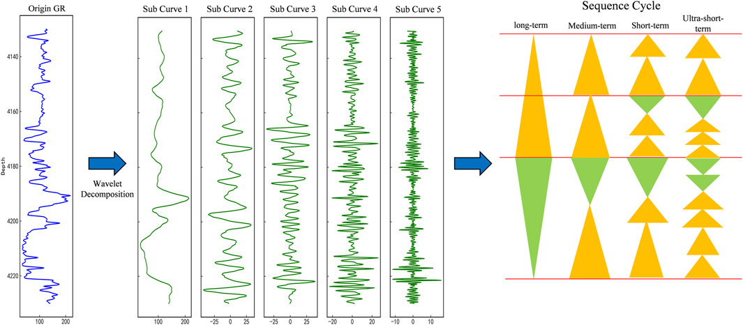
Figure 3. Analysis of stratigraphic depositional cycles based on wavelet-transformed logging curves. The original GR curve is decomposed into several sub-curves of different scales through wavelet transform. The low-frequency curve corresponds to long-term cycles, the medium-frequency curve corresponds to medium-term cycles, and the high-frequency curve corresponds to short-term cycles. The yellow upright triangle represents the positive cycle, while the green inverted triangle represents the negative cycle.

We employ the discrete wavelet transform (DWT) in conjunction with a multiresolution analysis (MRA) framework (Akansu and Haddad, 2001). For a given signal f(t), its representation at different resolution levels is constructed using wavelet functions and scaling functions to capture both detailed and abstract features. The fundamental principle of wavelet transform is to decompose a signal into components at various scales (frequencies). By selecting an appropriate wavelet basis function $\psi \left(t\right)$, the signal f(t) can be decomposed into low-frequency components (representing trends) and high-frequency components (representing details), the one-dimensional formula of discrete wavelet transform is given by Equation 1:

$\mathit{f}\left(\mathit{t}\right)={\displaystyle \sum _{\mathit{n}}}{C}_n{\psi }_n\left(t\right)(1)$

Where $c_n$ is the wavelet coefficient and ${\psi }_n\left(t\right)$ is the wavelet basis function of different scales. Multiresolution analysis builds upon this concept by progressively analyzing the signal at varying scales, from coarse to fine. At each scale, the signal is decomposed into a low-frequency component, capturing the overall trend, and a high-frequency component, representing fine-grained details. For a signal f(t), the multiresolution decomposition process can be described by Equation 2:

$f\left(t\right)={\displaystyle \sum _j}{\displaystyle \sum _k}{c}_{j,k}{\psi }_{j,k}\left(t\right)(2)$

where $c_{j,k}$ are the wavelet coefficients of the multiresolution analysis, and ${\psi }_{j,k}\left(t\right)$ is the wavelet basis function at scale j and position k. The signal f(t) is decomposed into low-frequency and high-frequency components at each level j. Assuming they are represented by $f{}_a{}^j\left(t\right)$ and $f{}_d{}^j\left(t\right)$, the original signal can be expressed as Equation 3:

$f\left(t\right)={\displaystyle \sum _j^J}{\displaystyle \sum _k}f{}_a{}^j\left(t\right)+{\displaystyle \sum _k}f{}_d{}^j\left(t\right)(3)$

In this study, the Daubechies ‘db4’ wavelet was selected as the basis function. The reason for this choice is its favorable properties for analyzing geological signals like well logs. The ‘db4’ wavelet is compactly supported and orthogonal, providing a good balance between time and frequency localization. Its shape is also well-suited for detecting abrupt changes and discontinuities in the log data, which often correspond to lithological boundaries or key stratigraphic surfaces. This makes it effective for decomposing the logs into components that are geologically meaningful.

This decomposition is based on wavelet coefficients and wavelet basis functions, used to separate components of different frequency bands in the signal, thereby analyzing the signal at different resolutions. Through layer-by-layer decomposition, the original signal can be reconstructed into multiple smooth curves, each representing the low-frequency characteristics of the signal at different resolutions. Then, we retain specific levels of components in the wavelet decomposition results and set the coefficients $c_{j,k}$ of other scales to zero. At this point, it can be used as a low-pass filter with resolution j. Further processing through the low-pass filter yields smooth curves with different time resolutions.

Through this method, the original logging curves are transformed into a multi-layer structure containing information at different scales, and the dimensionality of the input data changes from two-dimensional to three-dimensional (Figure 4). It should be noted that the training and validation sets in this study are based on single well, so there is no issue of data leakage.

Figure 4

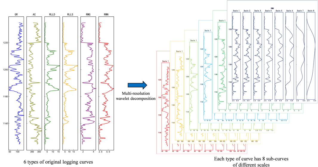
Figure 4. Decomposition of each original logging curve into multi-scale sub-curves using multiresolution wavelet decomposition. The training data is transformed from two-dimensional to three-dimensional.

The change of lithology is usually the comprehensive response of a section of logging curve (Park et al., 2022). The deep learning network model receives a sequence of length n as input, including continuous logging parameters such as resistivity and gamma ray. These parameters together constitute a multi-dimensional eigenvector that changes continuously with time. The goal of the model is to understand the pattern of these characteristics changing with time, and to predict the main lithology in the time period represented by the sequence. In order to more intuitively explain our model architecture and data processing process, Figure 5 shows how to divide the continuous logging data into multiple sequences with length N, and input each sequence as an independent sample into the LSTM network. Each sequence corresponds to a label, that is, the lithology predicted in this time period. In this way, our model can improve the accuracy and reliability of lithologic identification by using local patterns and global trends in time series.

Figure 5

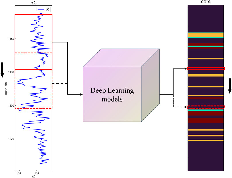
Figure 5. Mapping of logging time series segments to corresponding lithology labels through a deep learning model. When constructing the training set, a window of length n slides downward each time, and the lithology at the depth corresponding to the bottom of the window is used as the label.

3.2 Network structure

We propose a hybrid framework integrating 2DCNN and RNN, consisting of a channel-spatial attention-based residual network structure and a BiLSTM network. Two-dimensional convolutional neural networks are typically used in image processing tasks, while 1D convolutional kernels are commonly applied to time-series tasks to extract sequential features. Residual network (ResNet) are an innovative network structure in the field of deep learning in recent years, named after the introduction of skip connections (He et al., 2016). Compared to traditional two-dimensional convolutional neural networks, ResNet exhibits stronger expressive power in processing deep features. Through “skip connections” (Figure 6A), ResNet effectively alleviates the vanishing gradient problem in deep network training, allowing the network to learn deeper features without significantly increasing computational complexity. In logging lithology identification, logging curves after wavelet decomposition often exhibit complex nonlinear and hierarchical features. Using the ResNet model can more accurately extract these details. In contrast, traditional 2DCNN models may face information attenuation when processing deep features, while ResNet ensures information transmission through residual structures, thereby improving model classification accuracy and generalization ability.

Figure 6

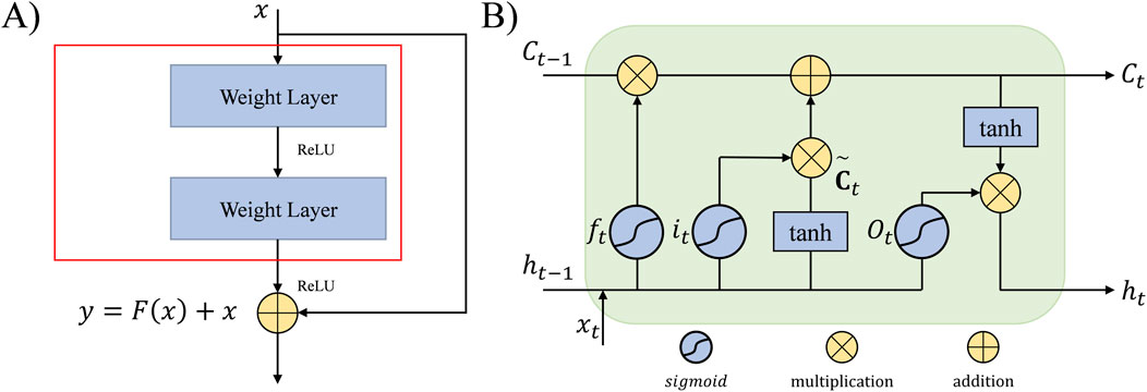
Figure 6. The structure of network: (A) residual network and (B) LSTM network.

For a given layer input x, with the output after two convolutional layers and activation as F(x), the output of the residual block is defined as Equation 4 (He et al., 2016):

$y=\mathrm{F}\left(x\right)+x(4)$

where F(x) represents the learned feature map, and x is the input carried over as the “shortcut connection.” This structure allows gradients to propagate efficiently, even in deep networks, reducing the risk of vanishing gradients.

To enhance global feature extraction in 2DCNN, we inserted a channel-spatial attention mechanism (CA) module between the two convolutional layers of the residual module (Liu N et al., 2021). The channel attention module amplifies cross-dimensional interactions, fully capturing different information for different logging curves, while the spatial attention module enhances the residual network’s ability to extract global features from multi-scale logging curves (Figure 2C). Here, M_c and M_s are the channel attention map and spatial attention map, respectively, F1 is the input feature, F2 is the intermediate state, and F3 is the output feature, defined as Equation 5 and Equation 6 (Liu Y et al., 2021):

${\mathrm{F}}_2={\mathrm{M}}_c\left({\mathrm{F}}_1\right)\otimes {\mathrm{F}}_1(5)$

${\mathrm{F}}_3={\mathrm{M}}_s\left({\mathrm{F}}_2\right)\otimes {\mathrm{F}}_2(6)$

Where $\otimes$ denotes element-wise multiplication. We constructed a three-layer residual neural network structure (Figure 6A). Unlike ResNet18 (He et al., 2016), considering the relatively small amount of input data from logging curves in the experiments, we chose 3 × 3 convolutional kernels for the convolutional layers, with a stride of 1 and padding of 1, replacing the original 7 × 7 large convolutional kernels, and the input feature maps are not downsampled. Additionally, the max-pooling layer was removed to retain as much original information as possible.

The long-term and short-term memory network (Hochreiter, 1997) is a special cyclic neural network (Figure 6B), which is specially used to process and learn the long-term dependence in sequential data. Traditional recurrent neural networks (RNN) are prone to vanishing or exploding gradients during backpropagation, but LSTM effectively solves this problem by introducing memory cells and gating mechanisms, allowing the network to “remember” or “forget” key information, thereby maintaining information flow in long sequence data. LSTM networks are used to process sequence data and remember important information over multiple time steps through gating mechanisms. The LSTM unit includes an input gate ${\mathrm{i}}_t$, a forget gate $f_t$, and an output gate $o_t$, with the following equations (Hochreiter, 1997):

${\stackrel{\sim }{\mathrm{C}}}_t=\tanh \left({\mathrm{W}}_C·\left[{\mathrm{h}}_{t-1},{\mathrm{x}}_t\right]+{\mathrm{b}}_C\right)(7)$

${\mathrm{C}}_t=\sigma \left({\mathrm{W}}_f·\left[{\mathrm{h}}_{t-1},{\mathrm{x}}_t\right]+{\mathrm{b}}_f\right)\times {\mathrm{C}}_{t-1}+\sigma \left({\mathrm{W}}_i·\left[{\mathrm{h}}_{t-1},{\mathrm{x}}_t\right]+{\mathrm{b}}_i\right)\times {\stackrel{\sim }{\mathrm{C}}}_t(8)$

${\mathrm{h}}_t=\sigma \left({\mathrm{W}}_o·\left[{\mathrm{h}}_{t-1},{\mathrm{x}}_t\right]+{\mathrm{b}}_o\right)\times \tanh \left({\mathrm{C}}_t\right)(9)$

In Equations 7–9, ${\mathrm{C}}_t$ and ${\mathrm{h}}_t$ represent the current cell state and hidden state, respectively, while ${\mathrm{C}}_{t-1}$ and ${\mathrm{h}}_t$ represent the cell state and hidden state from the previous time step. ${\stackrel{\sim }{\mathrm{C}}}_t$ denotes the current candidate cell state. W represents the weight matrices for the gates, and b represents the bias terms for the gates. σ and tanh denote the sigmoid activation function and the hyperbolic tangent activation function, respectively.

The BiLSTM network structure (Schuster and paliwal, 1997) is selected. It is composed of two LSTM layers, which extract temporal features from the positive and negative directions respectively, better grasp the long-term dependence of temporal features, and make up for the deficiency of two-dimensional convolution kernel of ResNet network. From the perspective of geological sedimentology, the strata are deposited from old to new, and the log lithology interpretation using BiLSTM network is more in line with the law of geological deposition. The parameters used in this study are shown in Figure 2A, including one BiLSTM layer with 128 hidden units.

3.3 Experiments

To prevent information leakage after applying wavelet transform, we divided the dataset into 8 training wells and 2 test wells, ensuring that the wells used for training and testing are independent. Additionally, since the ranges of each logging curve vary, it is necessary to normalize the six types of curves before training. In this study, we used the min-max normalization method (Equation 10), X represents the original data values to be normalized, such as the measured values in each well log curve, and min(X) and max(X) refer to the minimum and maximum values of the dataset, respectively. $X^{\prime }$ represents the normalized values, which will be scaled to between 0 and 1.

$X^{\prime }=\frac{X-X_{\mathit{min}}}{X_{\mathit{max}}-X_{\mathit{min}}}(10)$

During the training of the neural network model, we used the cross-entropy loss function, selected Adam as the optimizer, set the initial learning rate to 0.001, batch size to 16, and trained for 200 epochs (Table 2). The GPU was NVIDIA GeForce RTX 4060 Ti. To comprehensively evaluate the superiority of the proposed model, we designed four comparison models, described in Table 3, and compared the results of these five models. The comparison models included a Res-BiLSTM model without attention mechanisms, ResNet, BiLSTM, and LSTM models. Except for the architectural differences, the parameters of these comparison models were consistent with the proposed model. Note that BiLSTM and LSTM models used raw well log curves without wavelet decomposition as input, meaning the input data is two-dimensional.

Table 2

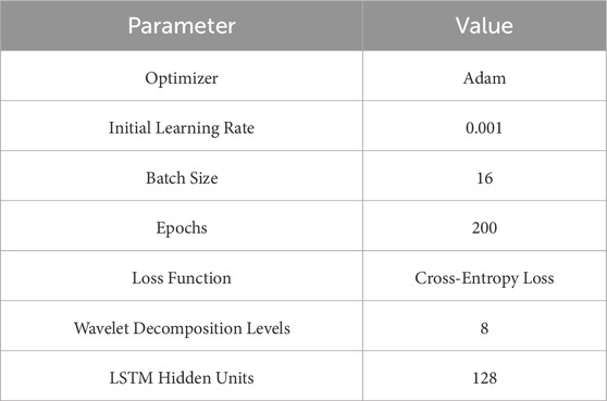
Table 2. Hyperparameters for the CA-HybridNet model training.

Table 3

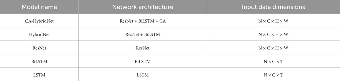
Table 3. Description of the proposed model and comparison models.

In machine learning experiments, the commonly used model evaluation indicators include accuracy, recall, F1 score and root mean square error (RMSE). For logging lithology interpretation task, precision and recall indexes of network model is equally important, so F1 score is used as the final evaluation index of the model, and its formula is as Equation 11:

$\mathrm{F}1-\mathrm{S}\text{cor}\mathrm{e}=\frac{2\times TP}{2\times TP+FP+FN}(11)$

Where TP represents the number of correctly classified positive samples, TN represents the number of correctly classified negative samples, FP represents the number of incorrectly classified negative samples, and FN represents the number of incorrectly classified positive samples. It is important to note that this study exclusively utilizes well log data for lithology identification.

4 Results

As shown in Figure 7, the training loss and accuracy curves of the five networks indicate that the three models incorporating the 2DCNN module (CA-HybridNet, HybridNet without the attention mechanism, and ResNet) exhibit significantly lower loss values compared to the BiLSTM and LSTM network models. Moreover, these three models achieve an accuracy rate of over 95% on the validation set. Further comparison of the performance of the two temporal network structures reveals that BiLSTM outperforms the LSTM network. This result fully demonstrates that the multi-scale logging curves processed by wavelet decomposition contain richer geological information. Using this data as training data for deep learning enables the network models to better extract the mapping relationships between logging curves and lithology. Compared to the BiLSTM and LSTM time series prediction models, the performance has been significantly improved. We counted the F1 scores of five models on the identification results of two wells, and the results showed that the performance of our proposed method was the best in both test wells.

Figure 7

Figure 7. Training loss (A) and accuracy (B) curves of the proposed and compared models. In both subplots, the red solid line, blue dashed line, green dotted line, orange dash-dot line, and purple solid line represent the CA-HybridNet, HybridNet, ResNet, BiLSTM, and LSTM models, respectively. The results demonstrate that the models incorporating 2DCNN modules converge faster and to lower loss values.

In the lithology identification results for Well 1 (Figure 8), CA-HybridNet, HybridNet, and ResNet achieved high accuracy. In the lithological interval from 1210 m to 1270m, these models demonstrated over 95% accuracy, particularly excelling in lithology transition zones (e.g., 1235–1245 m). Notably, ResNet failed to identify thin layers between 1275 and 1285 m, while HybridNet misclassified two thin layers at 1275 m. By contrast, CA-HybridNet accurately identified four thin layers at the bottom of Well 1, showcasing its superior capability in capturing thin-layer lithological features. Confusion matrix results further revealed that CA-HybridNet and HybridNet performed better in identifying siltstone and sandstone, whereas ResNet, lacking temporal sequence modules, had lower accuracy for shale predictions (Figure 9).

Figure 8

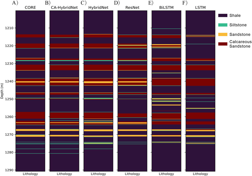
Figure 8. True lithology and prediction lithology results of five models on well 1: (A) True lithology, (B) CA-HybridNet, (C) HybridNet, (D) ResNet, (E) BiLSTM, and (F) LSTM.

Figure 9

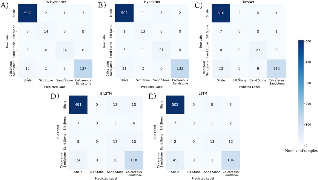
Figure 9. Confusion matrix of five models on well 1: (A) CA-HybridNet, (B) HybridNet, (C) ResNet, (D) BiLSTM, and (E) LSTM.

In Well 2, where thin layers were more prevalent (Figure 10), the performance differences between models became more pronounced. CA-HybridNet maintained the highest prediction accuracy despite some misclassifications near 1250 m. Overall, it outperformed other models, underscoring its strong lithology identification capabilities. The other four models exhibited significant errors in thin-layer regions, particularly in the 1,270–1300 m interval, where ResNet and LSTM performed poorly. These results highlight the superiority of CA-HybridNet in handling complex stratigraphic structures. For example, CA-HybridNet correctly identified nearly half of the siltstone samples, whereas the other four models showed poor performance, with a 0% success rate for siltstone identification in their confusion matrices (Figure 11).

Figure 10

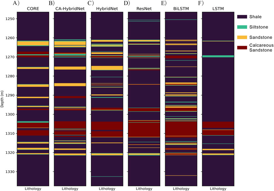
Figure 10. True lithology and prediction lithology results of five models on well 2: (A) True lithology, (B) CA-HybridNet, (C) HybridNet, (D) ResNet, (E) BiLSTM, and (F) LSTM.

Figure 11

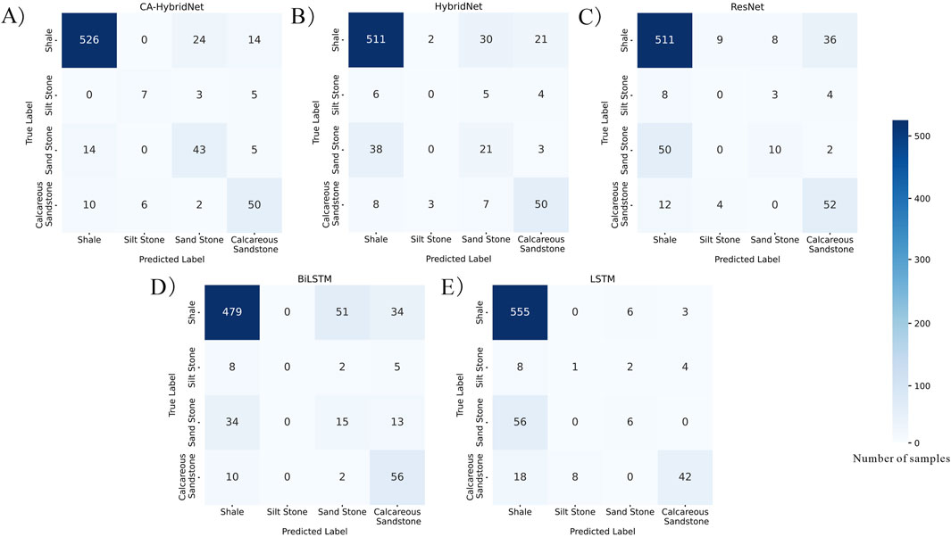
Figure 11. Confusion matrix of five models on well 2: (A) CA-HybridNet, (B) HybridNet, (C) ResNet, (D) BiLSTM, and (E) LSTM.

The imbalance in lithology sample distribution in the training and testing sets was also examined (Figure 12). In the training set and Well 1, shale accounted for approximately 72% of the samples, increasing to 80% in Well 2. Additionally, the proportion of sandstone and calcareous sandstone samples in Well 2 differed significantly from those in the training set and Well 1.

Figure 12

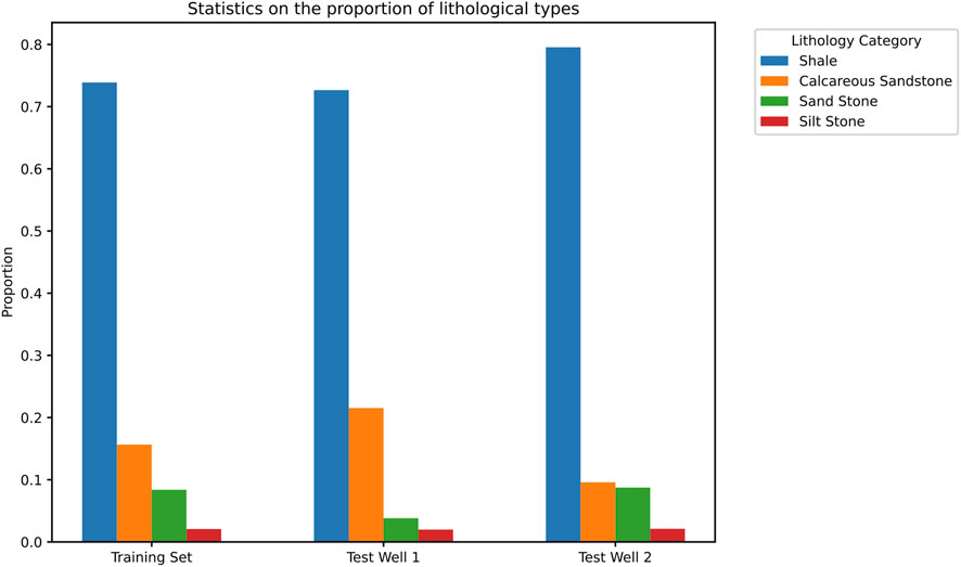
Figure 12. Proportion of lithology samples in the training set and testing wells. In the training set, well1 and well2, the number of samples from shale accounts for the vast majority. The number of samples from calcareous sandstone and sand stone ranges from 10% to 20%, while the number of samples from silt stone accounts for less than 5%. The proportion of lithological samples is highly imbalanced.

To investigate the impact of the number of well log curves generated by the multi-scale wavelet decomposition method on the results, additional experiments were conducted to examine the lithology interpretation accuracy when the well log curves were decomposed into 3 to 10 curves. As shown in Table 4, the model’s F1 score gradually increased with an increasing number of decomposed curves. Figure 13 presents the lithology identification results for different numbers of decomposed curves. The observations reveal that when fewer than 6 curves are decomposed, the model exhibits a higher error rate, with a noticeable error at 1,250 m; whereas, with more than 6 curves, this error is effectively mitigated. Notably, although using 10 decomposed curves resulted in improved lithology identification between 1,304 m and 1,312 m, it also led to an increased misclassification of lithologies as shale.

Table 4

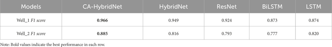
Table 4. F1 score of lithology prediction in two test wells using different models.

Figure 13

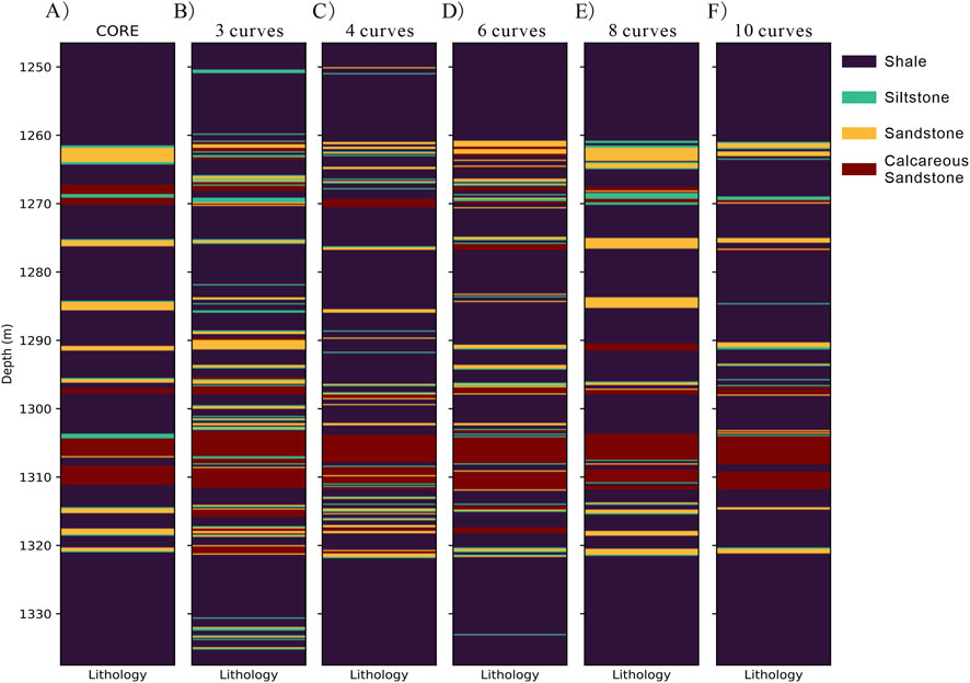
Figure 13. True lithology and prediction lithology results of different decomposition curves on well 2: (A) True lithology, (B) 3 curves, (C) 4 curves, (D) 6 curves, (E) 8 curves, and (F) 10 curves.

5 Discussion

These results demonstrate that the proposed CA-HybridNet significantly outperforms other baseline models, particularly in identifying thin-bedded lithologies and navigating complex stratigraphic transitions. This performance advantage can be attributed to the synergistic architecture: the wavelet decomposition provides a rich, multi-scale feature set, the 2D ResNet extracts geological patterns from these features, the bidirectional LSTM captures the crucial depth-dependent context, and the attention mechanism focuses the model on the most informative features. The bidirectional nature of the LSTM is particularly vital, as it allows the model to leverage both underlying and overlying strata information for prediction, mimicking how a geologist interprets logs within a stratigraphic sequence.

This study is conducted within a specific geological context of the Sanzhao Depression. We acknowledge that the model’s robustness has not yet been validated on data from entirely different geological basins, which remains an important direction for future work. However, the performance difference between Well 1 and Well 2 provides a valuable insight into the model’s generalization under conditions of ‘domain shift’. As shown in Figure 12, Well 2 exhibits a significantly different lithological distribution compared to the training set, with the proportion of shale increasing from 72% to 80%. This compositional shift explains the overall decrease in F1 scores for all models in Well 2. Critically, our proposed CA-HybridNet model demonstrated the most graceful degradation in performance and remained the top-performing model which F1 score is 0.885, significantly outperforming others. This suggests that by learning multi-scale geological features, our model has achieved a higher degree of robustness and is better equipped to handle natural geological variability compared to models that treat logs as simple 1D series.

Beyond the numerical improvement, it is important to interpret how the extracted “geological features” might reflect actual sedimentary processes. The wavelet-decomposed sub-curves provide a hierarchical view of the subsurface. The low-frequency components likely enable the model to identify macro-scale patterns, such as the gradual fining-upward sequence typical of a meandering channel migration, which might manifest as a slow, overarching trend in the logs. In contrast, the high-frequency components are essential for capturing sharp, localized events, such as the thin siltstone layers that represent crevasse splays or minor cyclic interfaces within a larger shale body. Traditional 1D models might smooth over these subtle, high-frequency details. Our hybrid architecture, by using a 2D CNN to process these multi-scale features, learns to recognize these complex patterns in a manner analogous to how a geologist interprets logs at different scales, thus moving beyond simple point-wise classification to a more context-aware interpretation. This aligns with recent advancements that leverage deep learning for complex subsurface characterization and reservoir performance prediction (Li et al., 2024; Deng et al., 2025).

Finally, the experiment on the number of decomposition curves (Table 5) indicates that more decomposition yields richer information up to a certain point (8 curves), after which performance may slightly decline due to potential redundancy or overfitting. This suggests that an optimal number of decomposition levels exists, likely related to the characteristic scales of geological heterogeneity in the study area. While our CA-HybridNet involves more parameters and higher training costs, the substantial improvement in accuracy and generalization, especially for economically significant thin reservoirs, justifies the additional computational expense. Future work could also explore integrating other data sources, such as seismic attributes or core data, leveraging techniques from related fields like rock physics (Zhang et al., 2024) and seepage characteristic analysis (Zhang et al., 2024), to further constrain the geological model and improve its physical realism.

Table 5

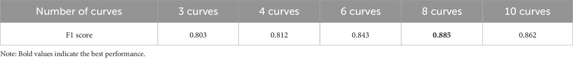
Table 5. F1 score of different decomposition curves on well 2.

6 Conclusion

This study proposes a novel geology-driven deep learning framework to address the critical challenge of accurately identifying thin-bedded lithologies from well logs. Our proposed CA-HybridNet architecture, designed around these geological principles, demonstrates superior performance over four baseline models in field data tests. This approach not only significantly improves identification accuracy but also exhibits enhanced generalization and robustness, maintaining high performance even on a test well that features a lithological distribution different from the training set. Overall, this work demonstrates that explicitly integrating geological principles into deep learning model design is a powerful strategy to improve lithology identification.

Data availability statement

The original contributions presented in the study are included in the article/supplementary material, further inquiries can be directed to the corresponding author.

Author contributions

LC: Methodology, Writing – original draft, Investigation, Data curation, Writing – review and editing, Conceptualization. XW: Supervision, Writing – review and editing, Conceptualization, Funding acquisition. ZL: Formal Analysis, Validation, Writing – original draft.

Funding

The author(s) declare that financial support was received for the research and/or publication of this article. This study is supported by National Natural Science Foundation of China (Grant No. 42074163).

Conflict of interest

The authors declare that the research was conducted in the absence of any commercial or financial relationships that could be construed as a potential conflict of interest.

Generative AI statement

The author(s) declare that no Generative AI was used in the creation of this manuscript.

Any alternative text (alt text) provided alongside figures in this article has been generated by Frontiers with the support of artificial intelligence and reasonable efforts have been made to ensure accuracy, including review by the authors wherever possible. If you identify any issues, please contact us.

Publisher’s note

All claims expressed in this article are solely those of the authors and do not necessarily represent those of their affiliated organizations, or those of the publisher, the editors and the reviewers. Any product that may be evaluated in this article, or claim that may be made by its manufacturer, is not guaranteed or endorsed by the publisher.

References

Akansu, A. N., and Haddad, R. A. (2001). Multiresolution signal decomposition: transforms, subbands, and wavelets. Academic Press.

Google Scholar

Ao, Y., Zhu, L., Guo, S., and Yang, Z. (2020). Probabilistic logging lithology characterization with random forest probability estimation. Comput. Geosciences 144, 104556. doi:10.1016/j.cageo.2020.104556

CrossRef Full Text | Google Scholar

Cao, Z., Xiong, Y., Xue, Y., Du, F., Li, Z., Huang, C., et al. (2025). Diffusion evolution rules of grouting slurry in mining-induced cracks in overlying strata. Rock Mech. Rock Eng., 1–20. doi:10.1007/s00603-025-04445-4

CrossRef Full Text | Google Scholar

Chang, J., Kang, Y., Zheng, W. X., Cao, Y., Wang, X. M., Lv, W., et al. (2021). Active domain adaptation with application to intelligent logging lithology identification. IEEE Trans. Cybern. 52 (8), 8073–8087. doi:10.1109/TCYB.2021.3049609

PubMed Abstract | CrossRef Full Text | Google Scholar

Deng, R., Dong, J., and Dang, L. (2025). Numerical simulation and evaluation of residual oil saturation in waterflooded reservoirs. Fuel 384, 134018. doi:10.1016/j.fuel.2024.134018

CrossRef Full Text | Google Scholar

Dev, V. A., and Eden, M. R. (2019). Formation lithology classification using scalable gradient boosted decision trees. Comput. Chem. Eng. 128, 392–404. doi:10.1016/j.compchemeng.2019.06.001

CrossRef Full Text | Google Scholar

dos Santos, D. T., Roisenberg, M., and dos Santos Nascimento, M. (2022). Deep recurrent neural networks approach to sedimentary facies classification using well logs. IEEE Geoscience Remote Sens. Lett. 19, 1–5. doi:10.1109/lgrs.2021.3053383

CrossRef Full Text | Google Scholar

Ehsan, M., Chen, R., Manzoor, U., Hussain, M., Abdelrahman, K., Khan, Z. U., et al. (2024). Unlocking thin sand potential: a data-driven approach to reservoir characterization and pore pressure mapping. Geomechanics Geophys. Geo-Energy Geo-Resources 10 (1), 160. doi:10.1007/s40948-024-00871-w

CrossRef Full Text | Google Scholar

Gao, Y., Tian, M., Grana, D., Xu, Z., and Xu, H. (2024). Attention mechanism-assisted recurrent neural network for well log lithology classification. Geophys. Prospect. 73, 628–649. doi:10.1111/1365-2478.13618

CrossRef Full Text | Google Scholar

He, K., Zhang, X., Ren, S., and Sun, J. (2016). “Identity mappings in deep residual networks,” in Computer Vision—eccv 2016. Editors B. Leibe, J. Matas, N. Sebe, and M. Welling (Cham, Switzerland: Springer International Publishing), 630–645. doi:10.1007/978-3-319-46493-0_38

CrossRef Full Text | Google Scholar

Hochreiter, S., (1997). Long short-term memory: neural computation MIT-press.

Google Scholar

Hong, Z., Yao, J., Li, K., and Hu, G. (2022). Conjunction of active and semi-supervised learning for wireline logs-based automatic lithology identification. IEEE Geoscience Remote Sens. Lett. 19, 1–5. doi:10.1109/LGRS.2022.3214929

CrossRef Full Text | Google Scholar

Hu, Q. H., Wang, C., Zhang, X., and Fan, J. J. (2015). Application of SOM neural network in lithology recognition. Appl. Mech. Mater. 713, 2169–2172. doi:10.4028/www.scientific.net/AMM.713-715.2169

CrossRef Full Text | Google Scholar

Jaikla, C., Devarakota, P., Auchter, N., Sidahmed, M., and Espejo, I. (2019). “FaciesNet: machine learning applications for facies classification in well logs,” in Conference on neural information processing systems (Vancouver: AAPG), 8–14.

Google Scholar

Jiang, C., Zhang, D., and Chen, S. (2021). Lithology identification from well-log curves via neural networks with additional geologic constraint. Geophysics 86 (5), IM85–IM100. doi:10.1190/geo2020-0676.1

CrossRef Full Text | Google Scholar

Kumar, T., Seelam, N. K., and Rao, G. S. (2022). Lithology prediction from well log data using machine learning techniques: a case study from talcher coalfield, eastern India. J. Appl. Geophys. 199, 104605. doi:10.1016/j.jappgeo.2022.104605

CrossRef Full Text | Google Scholar

Li, L., Wang, Z. Z., Yin, S. D., Wang, W. F., Yu, Z. C., Fan, W. T., et al. (2024). Selection and application of wavelet transform in high-frequency sequence stratigraphy analysis of coarse-grained sediment in rift basin. Petroleum Sci. 21 (5), 3016–3028. doi:10.1016/j.petsci.2024.06.020

CrossRef Full Text | Google Scholar

Li, Y., Jia, D., Wang, S., Qu, R., Qiao, M., and Liu, H. (2024). Surrogate model for reservoir performance prediction with time-varying well control based on depth generative network. Petroleum Explor. Dev. 51 (5), 1287–1300. doi:10.1016/S1876-3804(25)60541-6

CrossRef Full Text | Google Scholar

Lin, J., Li, H., Liu, N., Gao, J., and Li, Z. (2020). Automatic lithology identification by applying LSTM to logging data: a case study in X tight rock reservoirs. IEEE Geoscience Remote Sens. Lett. 18 (8), 1361–1365. doi:10.1109/LGRS.2020.3001282

CrossRef Full Text | Google Scholar

Liu N, N., Huang, T., Gao, J., Xu, Z., Wang, D., and Li, F. (2021). Quantum-enhanced deep learning-based lithology interpretation from well logs. IEEE Trans. Geoscience Remote Sens. 60, 1–13. doi:10.1109/TGRS.2021.3085340

CrossRef Full Text | Google Scholar

Liu Y, Y., Shao, Z., and Hoffmann, N. (2021). Global attention mechanism: retain information to enhance channel-spatial interactions. arXiv Prepr. arXiv:2112.05561. doi:10.48550/arXiv.2112.05561

CrossRef Full Text | Google Scholar

Lv, H., Ma, L., Li, H., Wen, X., Wu, B., and Gao, J. (2024). Strata-constrained gaussian window weighted-constrained long short-term memory network for logging lithology prediction. Interpretation 12 (3), SE15–SE24. doi:10.1190/INT-2023-0062.1

CrossRef Full Text | Google Scholar

Manzoor, U., Ehsan, M., Hussain, M., and Bashir, Y. (2024). Improved reservoir characterization of thin beds by advanced deep learning approach. Appl. Comput. Geosciences 23, 100188. doi:10.1016/j.acags.2024.100188

CrossRef Full Text | Google Scholar

Mohammadi, K., Mousavi, S. H. R., Hosseini-Nasab, S. M., and Shahbazi, M. (2025). Transforming petrophysical well-logs to images: leveraging deep learning for lithology recognition. Earth Sci. Inf. 18 (3), 457–23. doi:10.1007/s12145-025-01953-3

CrossRef Full Text | Google Scholar

Mukherjee, B., Kar, S., and Sain, K. (2024). Machine learning assisted state-of-the-art-of petrographic classification from geophysical logs. Pure Appl. Geophys. 181 (9), 2839–2871. doi:10.1007/s00024-024-03563-4

CrossRef Full Text | Google Scholar

Pang, Q., Chen, C., Sun, Y., and Pang, S. (2024). STNet: advancing lithology identification with a spatiotemporal deep learning framework for well logging data. Nat. Resour. Res. 34, 327–350. doi:10.1007/s11053-024-10413-6

CrossRef Full Text | Google Scholar

Park, G. T., Jeong, J., Emelyanova, I., Pervukhina, M., Esteban, L., and Yun, S. T. (2022). Data-driven sequence labeling methods incorporating the long-range spatial variation of geological data for lithofacies sequence estimation. J. Petroleum Sci. Eng. 208, 109345. doi:10.1016/j.petrol.2021.109345

CrossRef Full Text | Google Scholar

Ren, Q., Zhang, D., Zhao, X., Yan, L., and Rui, J. (2022). A novel hybrid method of lithology identification based on k-means++ algorithm and fuzzy decision tree. J. Petroleum Sci. Eng. 208, 109681. doi:10.1016/j.petrol.2021.109681

CrossRef Full Text | Google Scholar

Saporetti, C. M., da Fonseca, L. G., and Pereira, E. (2019). A lithology identification approach based on machine learning with evolutionary parameter tuning. IEEE Geoscience Remote Sens. Lett. 16 (12), 1819–1823. doi:10.1109/LGRS.2019.2911473

CrossRef Full Text | Google Scholar

Schuster, M., and Paliwal, K. K. (1997). Bidirectional recurrent neural networks. IEEE Trans. Signal Process. 45 (11), 2673–2681. doi:10.1109/78.650093

CrossRef Full Text | Google Scholar

Song, M. H., Won, C. D., Chae, C. H., and Paek, N. I. (2021). Spectral analysis based on wavelet transform maxima: identification of multi-order stratigraphic boundaries and cycles. Math. Geosci. 53, 969–997. doi:10.1007/s11004-020-09879-w

CrossRef Full Text | Google Scholar

Sun, S., Shu, L., Zeng, Y., Cao, J., and Feng, Z. (2007). Porosity–permeability and textural heterogeneity of reservoir sandstones from the Lower Cretaceous putaohua member of yaojia formation, weixing oilfield, songliao basin, northeast China. Mar. Petroleum Geol. 24 (2), 109–127. doi:10.1016/j.marpetgeo.2006.10.006

CrossRef Full Text | Google Scholar

Sun, L., Li, Z., Li, K., Liu, H., Liu, G., and Lv, W. (2023). Cross-well lithology identification based on wavelet transform and adversarial learning. Energies 16 (3), 1475. doi:10.3390/en16031475

CrossRef Full Text | Google Scholar

Teng, T., Chen, Y., Wang, Y., and Qiao, X. (2025). In situ nuclear magnetic resonance observation of pore fractures and permeability evolution in rock and coal under triaxial compression. J. Energy Eng. 151 (4), 04025036. doi:10.1061/jleed9.eyeng-6054

CrossRef Full Text | Google Scholar

Wang, J., and Cao, J. (2023). A lithology identification approach using well logs data and convolutional long short-term memory networks. IEEE Geoscience Remote Sens. Lett. 20, 1–5. doi:10.1109/LGRS.2023.3322677

CrossRef Full Text | Google Scholar

Wang, X., Yang, S., Zhao, Y., and Wang, Y. (2018). Lithology identification using an optimized KNN clustering method based on entropy-weighed cosine distance in Mesozoic strata of gaoqing field, jiyang depression. J. Petroleum Sci. Eng. 166, 157–174. doi:10.1016/j.petrol.2018.03.034

CrossRef Full Text | Google Scholar

Wang, J., Cheng, S., Tian, J., and Gao, Y. (2023). A 2D CNN-LSTM hybrid algorithm using time series segments of EEG data for motor imagery classification. Biomed. Signal Process. Control 83, 104627. doi:10.1016/j.bspc.2023.104627

CrossRef Full Text | Google Scholar

Wang, R., Wang, G., Zhao, G., Qian, M., Liu, Y., He, W., et al. (2023). Geological characteristics and resources potential of shale oil in chang 7 member of Upper Triassic yanchang formation in Fuxian area, southern ordos basin, Western China. Unconv. Resour. 3, 237–247. doi:10.1016/j.uncres.2023.06.001

CrossRef Full Text | Google Scholar

Wang, R., Liu, Y., Li, Z., Wang, D., Wang, G., Lai, F., et al. (2024). Microscopic pore structure characteristics and controlling factors of marine shale: a case study of Lower Cambrian shales in the southeastern Guizhou, upper yangtze platform, south China. Front. Earth Sci. 12, 1368326. doi:10.3389/feart.2024.1368326

CrossRef Full Text | Google Scholar

Wang, L., Zhang, W., Cao, Z., Xue, Y., and Xiong, F. (2025). Coupled effects of the anisotropic permeability and adsorption-induced deformation on the hydrogen and carbon reservoir extraction dynamics. Phys. Fluids 37 (6), 066608. doi:10.1063/5.0270765

CrossRef Full Text | Google Scholar

Xu, S., Chen, S., Xue, J., and Kong, L. (2023). Construction technology of superimposition patterns of sandbodies driven by well-seismic data and its application: taking the putaohua reservoir of yaojia formation in the northeastern WX oilfield as an example. Oil Geophys. Prospect. 58 (1), 178–189. doi:10.13810/j.cnki.issn.1000-7210.2023.01.019

CrossRef Full Text | Google Scholar

Yu, Z., Wang, Z., and Wang, J. (2023). Continuous wavelet transform and dynamic time warping-based fine division and correlation of glutenite sedimentary cycles. Math. Geosci. 55 (4), 521–539. doi:10.1007/s11004-022-10039-5

CrossRef Full Text | Google Scholar

Zhang, G., Wang, Z., and Chen, Y. (2018). Deep learning for seismic lithology prediction. Geophys. J. Int. 215 (2), 1368–1387. doi:10.1093/gji/ggy344

CrossRef Full Text | Google Scholar

Zhang, L., Luo, L., Pan, J., Li, X., Sun, W., and Tian, S. (2024). Seepage characteristics of coal under complex mining stress environment conditions. Energy and Fuels 38 (17), 16371–16384. doi:10.1021/acs.energyfuels.4c02870

CrossRef Full Text | Google Scholar

Zhang, L., Yuan, X., Luo, L., Tian, Y., and Zeng, S. (2024). Seepage characteristics of broken carbonaceous shale under cyclic loading and unloading conditions. Energy and Fuels 38 (2), 1192–1203. doi:10.1021/acs.energyfuels.3c04160

CrossRef Full Text | Google Scholar

Zhu, L., Li, H., Yang, Z., Li, C., and Ao, Y. (2020). Intelligent logging lithological interpretation with convolution neural networks: petrophysics: the SPWLA journal of formation. Eval. Reserv. Descr. 59 (6), 799–810. doi:10.30632/PJV59N6-2018a5

CrossRef Full Text | Google Scholar