Abstract
Introduction:
Rocks are subjected to pressure and temperature underground. In situ mechanical properties of organic shales are of principal importance in unconventional reservoir exploration and production, CO2 sequestration, and geothermal energy exploitation.
Methods:
To better understand the combined effects of temperature and confining pressure on anisotropic mechanical properties, we perform a series of triaxial tests on two pairs of organic shales at temperatures ranging from 25 °C to 105 °C and confining pressures varying from 5 MPa to 45 MPa. Both static and dynamic mechanical properties (Young’s modulus and Poisson’s ratio) are investigated.
Results:
The experimental results suggest that the increasing confining pressure and temperature increase and decrease dynamic Young’s moduli, respectively, but jointly increase the apparent static Young’s moduli. The temperature effect on dynamic properties is weakened, while that on static properties is increased by the increasing confining pressure. In contrast, an increase in temperature increases confining pressure effects on both dynamic and static properties. Additionally, due to the existence of bedding planes, compaction and thermal expansion caused by the increasing confining pressure and temperature are anisotropic. With increased confining pressure, the anisotropy of dynamic properties decreases while that of static properties increases, with a tendency to approach each other at the maximum confining pressure. However, the anisotropies of dynamic and static properties tend to diverge from each other with increasing temperature. Moreover, although dynamic properties are characteristically greater than static ones, the correlation coefficients between dynamic and static Young’s moduli are highly affected by the applied confining pressure and temperature. Ignoring either effect would result in an overestimation of the correlation coefficient.
Discussion:
The findings provide an innovative approach to jointly evaluate the effects of temperature and confining pressure effects on dynamic–static correlations in anisotropic shales, although limited samples and measurement constraints might create limitations in geoengineering applications.
1 Introduction
Understanding the in situ mechanical properties of organic-rich reservoir shales is of considerable significance in numerous geoengineering applications, such as unconventional reservoir exploration and production (Zhao et al., 2016), environmental geomechanics (Castelletto et al., 2013), geothermal energy, greenhouse gas sequestration (Arif et al., 2017), and deep mining. Mechanical properties of rock materials, like Young’s modulus and Poisson’s ratio, could be determined by either the stress–strain relation (i.e., static measurement) or the propagating elastic wave velocities (i.e., dynamic measurement). Both dynamic and static properties are sensitive to the ambient environment subjected to rocks, such as confining pressure and temperature (Vernik and Nur, 1992; Niandou et al., 1997; Sone and Zoback, 2013; Blake and Faulkner, 2016). The primary focus of this study is to systematically explore the combined effects of confining pressure and temperature on both dynamic and static properties of anisotropic shales.
The pressure and temperature effects on rock properties have long been investigated from the dynamic (Mobarak and Somerton, 1971; Timur, 1977; Johnston, 1987; Wang and Nur, 1988) or static (Jones and Nur, 1983; Hassanzadegan et al., 2012; Masri et al., 2014; Zhang et al., 2015; Herrmann et al., 2018) perspective. From a dynamic aspect, a general conclusion is that ultrasonic velocities or dynamic moduli increase with increasing confining pressure and decrease with increasing temperature. The pressure dependence of dynamic properties is typically attributed to microcrack closure and changes in grain-to-grain contact (King, 1966; Wang et al., 2020a), whereas the temperature dependence is caused by softening of mineral grains or grain boundaries (Kern, 1978; Wang and Nur, 1988; Hassanzadegan et al., 2012). Nevertheless, the confining pressure and temperature dependencies of static mechanical properties are complex. Masri et al. (2014) conducted triaxial compression tests on Tournemire shales at different confining pressures while increasing temperatures up to 250 °C. They observed significant decreases in the static Young’s modulus with increasing temperature. Herrmann et al. (2018) performed deformation tests on Posidonia and Bowland shales at both ambient and in situ conditions. They found that the static Young’s modulus and compressive strength are strongly dependent on the confining pressure, while the rising temperature only has a minor influence on them.
Correlations between in situ dynamic and static mechanical properties are of great significance in many geoengineering applications, like wellbore stability, hydraulic fracturing, and reservoir modeling (Barree et al., 2009; Sone and Zoback, 2013; Vernik, 2016). Many scholars focus on investigating the mismatch between dynamic and static properties. The differences between dynamic and static elasticity are frequently attributed to the variations in strain amplitude (Walsh, 1965; Ong et al., 2016; Fjær, 2019; Gong et al., 2019; Wang et al., 2020a; Wang et al., 2020b). The strain amplitude induced by the applied stress during static tests ranges from 10−5 to 10−3, which is greater than that produced by propagating elastic waves (10−8 to 10−6) by several orders of magnitude (Fjær, 2019). However, little data address the combined pressure–temperature effects on the dynamic–static mechanical relationships. To precisely establish dynamic–static property correlations in the laboratory, two significant factors associated with geological processes, confining pressure and temperature, should be considered. Many researchers (Asef and Najibi, 2013; Meléndez-Martínez and Schmitt, 2016; Ramos et al., 2019; Blake et al., 2020) have discussed the potential roles of the applied confining pressure in dynamic–static property correlations. However, little research has been conducted in relation to temperature effects on dynamic–static property correlations, let alone the combined effects of confining pressure and temperature.
Organic shales are anisotropic, with a finely laminated texture with clay platelets, microcracks, and lenticular kerogen particles (Vernik and Nur, 1992; Dewhurst and Siggins, 2006; Zhao et al., 2016; Ramos et al., 2019). The presence of laminae or beddings in shales would result in pronounced anisotropy in both mechanical and thermal behaviors. Meléndez-Martínez and Schmitt (2016) measured anisotropic Young’s moduli of four shale samples at confining pressures up to 60 MPa and concluded that the Young’s modulus perpendicular to the bedding plane is more pressure-sensitive than that parallel to the bedding plane. With the increased confining pressure, the anisotropy degree gradually decreases to an asymptotic value, which defines the intrinsic anisotropy (Vernik, 2016). Additionally, some previous studies have demonstrated that the thermal expansion of rocks is anisotropic due to different mineral compositions and the presence of bedding planes (Somerton, 1992; Ding et al., 2020; Gabova et al., 2020). One consensus is that the axial expansion coefficient of samples with horizontal foliation is larger than that of samples with vertical foliation (Zhang et al., 2015; Herrmann et al., 2018; Gabova et al., 2020). These unequal expansions can be expected to cause microcracks preferentially in the direction along bedding planes (Zhou et al., 2016). As a result, due to the complex structure of anisotropic shales, the anisotropy degree will inevitably vary with the applied confining pressure and temperature.
To our best knowledge, no measurements, whether dynamic or static, have been performed to quantify the anisotropy evolution with temperature and confining pressure simultaneously. Ignoring the effects of anisotropy will give rise to significant errors in seismic surveys, well-log interpretations, and micro-seismic monitoring (Sone and Zoback, 2013), as well as geomechanical applications in drilling and hydraulic-fracture designing (Vernik, 2016).
In this study, a suite of triaxial tests is performed on two pairs of organic shales at varied confining pressure and temperature conditions. We aim to discuss the combined effects of confining pressure and temperature on the mechanical properties of anisotropic shales from both dynamic and static aspects. Additionally, the combined pressure–temperature effects on mechanical properties in directions perpendicular and parallel to bedding planes are comparatively analyzed, intending to evaluate the anisotropy evolution with varied confining pressure and temperature. Moreover, the nature of physical mechanisms responsible for the thermomechanical properties of organic shales is investigated via analysis of thin sections and scanning electron microscopy (SEM). Finally, we discuss correlations between dynamic and static Young’s modulus and potential errors caused by ignoring the confining pressure or temperature effect.
2 Experiments and methods
2.1 Sample characterizations
Two full-diameter (6-inch) shale cores, defined as #Y3 and #Y4, were acquired from an unconventional oil shale play with a lacustrine depositional environment, located in Northeastern China. The burial depth of #Y3 and #Y4 shales was 2,557.86 m and 2,554.96 m, respectively. The cores have visible depositional bedding planes. To investigate the anisotropic mechanical properties of organic shales, two cylindrical specimens (Figure 1) were cut from each full-diameter core with directions perpendicular (“V”) and parallel (“H”) to the bedding plane, respectively. The ends of each specimen were ground flat. According to the ISRM suggested methods in 1983 (Kovari et al., 1983), all four cylindrical specimens (“#Y3_V”, “#Y3_H”, “#Y4_V”, “#Y4_H”) were machined to have a diameter of 2.54 cm and a length–diameter ratio of 2.0. The clay content of the selected shales is beyond 25%, as shown in Table 1. Adsorbed inter-layer and inter-particle bonded water of clay minerals are unavoidable, which might result in pore pressure buildup during the fast stress loading and subsequent overestimation of the mechanical properties (Ewy, 2018; Schuster et al., 2021; Crisci et al., 2022). In the current study, we dried four shale specimens in an electric vacuum oven at 60 °C for ∼24 h (ISRM, 2007; Kiuru et al., 2023). The rock mass was recorded every 4 h until the variation of rock mass was within ±0.01 g. The bulk density was derived from the dry specimen weight and volume. The bulk density is 2.48 g/cm3 and 2.47 g/cm3 for #Y3_V and #Y3_H, respectively, and 2.45 g/cm3 and 2.44 g/cm3 for #Y4_V and #Y4_H, respectively. The grain density and porosity were measured with the helium porosimeter based on Boyle–Mariott’s law. Porosities in two directions are 4.2% and 4.4% for #Y3, and 5.3% and 5.1% for #Y4. The similarity of bulk density and porosity in two orthogonal directions indicates that the selected pairs of shale samples are relatively homogeneous. Additionally, the residual cutting shale powders were used for the X-ray diffraction (XRD) analysis, which revealed that the selected shale is a mixture of quartz, feldspar, calcite, dolomite, pyrite, and clay. The total carbon content (TOC) was obtained via the pyrolysis test, as shown in Table 1.
FIGURE 1

Coring principle from a full-diameter shale sample with a transversely isotropic structure. In the X1/X2/X3 coordinate system, strains and velocities measured on vertical (V) and horizontal (H) specimens are shown.
TABLE 1
| Sample | Clay (vol.%) | Quartz (vol.%) | Feldspar (vol.%) | Calcite (vol.%) | Dolomite (vol.%) | Pyrite (vol.%) | TOC (wt.%) |
|---|---|---|---|---|---|---|---|
| #Y3 shale | 27.5 | 32 | 29.5 | 3.5 | 5.5 | 2 | 1.73 |
| #Y4 shale | 28.6 | 24.8 | 7.3 | — | 38.1 | 1.2 | 1.93 |
Mineral compositions of #Y3 and #Y4 shales according to the XRD analysis.
Figures 2, 3 show the thin section and scanning electron microscopy (SEM) images for #Y3 and #Y4 in directions perpendicular and parallel to bedding planes, respectively. Figures 2b, 3b show that clay minerals constitute the main matrix of the rock, while solid grains are distributed in a dispersed manner. Figures 2a,c, 3a,c show that the solid grains of #Y3 shale are dominated by siliceous minerals, like quartz or feldspar, while dolomite minerals can be seen in #Y4 shale, which is in accordance with the results of XRD analysis in Table 1. As shown in Figures 2d, 3d, clay minerals are aligned in the direction sub-parallel to bedding planes, indicating a transversely isotropic structure (Wang et al., 2021a). Black organic matter is intertwined with clay and solid grains and shows a preferred orientation along the bedding plane. The kerogen exhibits a lenticular texture with visible organic pores. Additionally, although shales are quite consolidated, it is unavoidable to create intergranular or intragranular microcracks during core recovery due to stress relief and cooling (Li and Schmitt, 1998). Such microcracks in the selected shales are preferentially aligned in directions sub-parallel to bedding planes.
FIGURE 2

Thin-section images for (a) the vertical and (b) the horizontal #Y3 shale sample; SEM images for (c) the vertical and (d) the horizontal #Y3 shale sample. Note: both thin-section and SEM images are taken from the top surface of cylindrical samples.
FIGURE 3

Thin-section images for (a) the vertical and (b) the horizontal #Y4 shale sample; SEM images for (c) the vertical and (d) the horizontal #Y4 shale sample. Note: both thin-section and SEM images are taken from the top surface of cylindrical samples.
2.2 Experimental setups
We employ a servo-controlled triaxial testing system (AutoLab 1500, manufactured by the New England Research) to conduct dynamic and static tests simultaneously at various confining pressures and temperatures. As shown in Figure 4, the experimental setup is composed of a stress–strain measurement system, an ultrasonic velocity measurement system, and a temperature measurement system (Wang et al., 2021b).
FIGURE 4

Schematic of the servo-hydraulically controlled triaxial testing system.
Axial load is measured using an internal load cell with a maximum capacity of 832 kN. Axial stresses calculated from measured forces are corrected from the previous calibration runs with a standard aluminum. The confining pressure is applied by pumping hydraulic oil into the vessel. The pressure can be increased to 68 MPa by a servo-controlled high-pressure generator. As shown in Figure 4, the rock sample is fixed together with two titanium stacks using a Viton rubber jacket. The axial strain (εa) is recorded by mounting a pair of linear variable differential transformers (LVDTs) between the top and bottom platens. The radial strain (εr) is measured by placing another LVDT at the middle of the sample. The precision of strain measurements is approximately 0.01 μm. At the very beginning, the LVDTs and strains are calibrated, considering that the triaxial framework would create strains during the axial compression. Given that the selected shales have a transversely isotropic structure, as shown in Figure 1, the axial strains measured in the vertical and horizontal samples are perpendicular and parallel to bedding planes, defined as εa3 and εa1, respectively. The radial strain in the vertical sample is parallel to the bedding plane, defined as εr1. While measuring the horizontal sample, the radial LVDT is fixed in the direction perpendicular to the bedding plane. In this case, the measured radial strain is defined as εr3. It is pertinent to mention that errors in axial strain induced by titanium stacks have been calibrated by measuring a standard aluminum before measuring rock samples.
Ultrasonic velocity measurements are achieved by embedding tablet-shaped piezoelectric transducers (PZTs) inside the top and bottom platens, acting as transmitters and receivers, respectively. As shown in Figure 4, the acoustic PZTs include a pair of P-wave transducers with a central frequency of 0.75 MHz and two pairs of S-wave transducers (e.g., pure-shear mode (SH) and quasi-shear mode (SV)) with a central frequency of 0.45 MHz. Before the measurements, the travel times created by the platen buffers are calibrated by keeping the two platens in contact. Accordingly, P- and S-wave velocities are calculated with the strain-calibrated sample length divided by the P- and S-wave first arrivals from the pulse transmission signals. The precision of velocity measurements is approximately ±1% and ±2% for P- and S-waves, respectively. P-wave velocities measured in the vertical and horizontal samples are defined as vP (0°) and vP (90°), respectively, as shown in Figure 1. The S-wave velocity measurement made in the vertical sample represents a pure SH mode propagating perpendicular to the bedding plane and polarizing parallel to the bedding plane, defined as vS (0°). In the horizontal sample, two S-wave measurements represent a pure SH mode polarizing in the bedding-parallel and an SV mode polarizing in the bedding-normal directions, respectively, referred to as vSH(90°) and vSV(90°), respectively.
The heating of the sample is executed using three heater bands around the external wall of the confining cell, as shown in Figure 4. A thermocouple is mounted in the vicinity of the heater bands to record the temperature. The heating system has a temperature capacity of 120 °C. The confining cell with heater elements is jacketed with an insulation layer during the measurements. Three heater bands heat the hydraulic oil inside the cell, which in turn heats the sample. To precisely control the temperature inside the confining vessel, a second thermocouple is installed in the vicinity of the sample, as shown in Figure 4. The recorded temperature by the second thermocouple is fed back to the data acquisition system. The uncertainty of the recorded temperature is ±1 °C.
2.3 Experimental procedures and methods
After placing the sample assemblage inside the confining cell, a series of multi-stage compressive tests to collect experimental measurements is conducted at five temperature levels: 25 °C, 45 °C, 65 °C, 85 °C, and 105 °C. At each temperature, the confining pressure is stepwise loaded to 5 MPa, 15 MPa, 25 MPa, 35 MPa, and 45 MPa, respectively, with a loading rate of 0.689 MPa/s. At each confining pressure level, two deviatoric cycling tests with a stress magnitude of 10 MPa are carried out with a loading rate of 0.345 MPa/s at five confining pressure conditions. It should be noted that the ultrasonic velocities are measured at five confining pressure conditions before the deviatoric stresses are applied. Having completed measurements at a temperature level, the temperature is stepwise increased to the next level. The maximum confining pressure (45 MPa) and temperature (105 °C) are set to roughly simulate in situ conditions at a 2–3 km depth. The temperature, confining pressure, deviatoric stress, and axial and radial strains are continuously recorded, taking #Y3 shale in Figure 5 for example. The recorded strains are caused by variations of both stress and temperature.
FIGURE 5
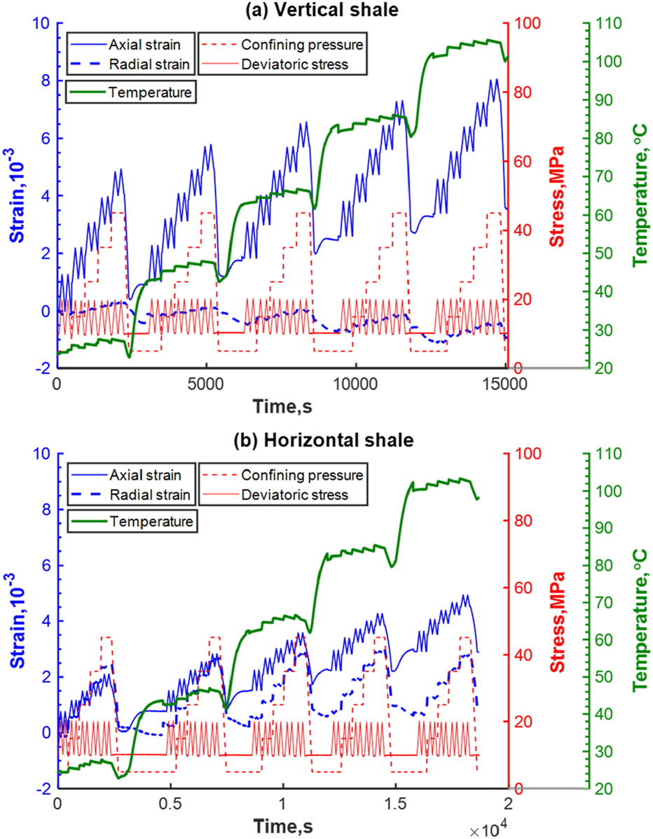
Evolutions of confining pressure (pc), deviatoric stress (σd), axial strain (εa), radial strain (εr), and temperature (T) with time, taking (a) the vertical and (b) the horizontal #Y3 shale as the example.
When the deviatoric stress is initially applied, the stress–strain curves would show some nonlinearity given the closure of microcracks or compliant pores (Wang et al., 2020b; Ren et al., 2021). In addition, hysteresis of the stress–strain curves (black symbols in Figure 6) between stress load and unload is unavoidable, which would subsequently affect the determination of static elastic properties (Wang et al., 2022). As a result, we set two deviatoric stress cycles with a stress amplitude of 10 MPa to minimize the effects of nonlinearity and hysteresis. The static Young’s modulus is derived by linearly fitting the axial strain–stress curve in the second deviatoric stress cycle (blue circles in Figure 6a) at each temperature and confining pressure level. The static Poisson’s ratio is determined in a similar way using curves between radial and axial strains (blue squares in Figure 6b). Additionally, static elastic modulus in rock mechanics is defined as the relationship between the applied stress and the strain induced by the applied stress. In the current study, the static elastic modulus describes the relation between the applied stress and the strain caused by both the applied stress and the temperature. Therefore, the static elastic properties are defined as “the apparent static elastic properties” in the current study. The apparent static Young’s moduli are expressed with E33stapparent and E11stapparent, whereas the apparent static Poisson’s ratios are defined as ν31stapparent and ν13stapparent for vertical and horizontal shales, respectively.
FIGURE 6

Methods for deriving static Young’s modulus (a) and Poisson’s ratio (b), respectively, taking #Y3_V shale at the confining pressure of 45 MPa and the temperature of 85 °C as the example. The slopes of linearly fitting εa-σd and εa-εr curves in cycle 2 are considered to be the static Young’s modulus and Poisson’s ratio.
Additionally, Young’s modulus and Poisson’s ratio of rock materials could be determined by the measured bulk density and elastic wave velocities. For shales with transversely isotropic structure, the relationship between stresses and strains can be characterized with five independent stiffness constants (c11, c33, c44, c66, and c13) according to the anisotropic Hooke’s law (Lo et al., 1986; Mavko et al., 2009). Subsequently, two dynamic Young’s moduli (i.e., E33dyn and E11dyn) and three dynamic Poisson’s ratios (i.e., ν31dyn, ν13dyn, and ν12dyn) are expressed with five stiffnesses according to Equations 1–5:
To obtain five stiffnesses for the complete identification of the transversely isotropic tensor, at least one P-wave velocity in the non-principal direction (e.g., at 45° to the symmetry axis X3) is necessary, in addition to P- and S-wave velocities at 0° and 90° to the X3-axis (Vernik, 2016). c11, c33, c44, c66 are calculated according to Equations 6–9. Limited by the acoustic measurement system in this study, no off-axis P-wave velocity can be measured. Yan et al. (2019) proposed an empirical c13 prediction model, which uses data points from classical literature (Thomsen, 1986; Johnston and Christensen, 1995; Wang, 2002; Sone and Zoback, 2013; Vernik, 2016). Data points used for modeling are also checked by the upper and lower bounds proposed by Chichinina and Vernik (2018). Hence, we use Equation 10 (the empirical c13 prediction equation) to realize the calculations of the complete set of mechanical parameters.
3 Experimental results
3.1 Dynamic properties of anisotropic shales
Figure 7 shows P-wave velocities (vP (0°) and vP (90°)) and S-wave velocities (vS (0°) and vSH(90°)) as functions of the confining pressure (pc) and temperature (T) for two pairs of shale samples (#Y3 and #Y4 shale). Overall, for each pair of shales, vP (90°) > vP (0°) and vSH (90°) > vS (0°) are always satisfied at any confining pressure or temperature levels, indicating the transversely isotropic structure for the selected shales. Four ultrasonic velocities linearly increase with the increasing confining pressure at any temperature condition without exhibiting the curvature normally seen in sandstones (Johnston, 1987). The velocity increase over the applied pressure range tends to increase somewhat with the elevated temperature. The velocity decrements at five temperatures are averaged to compare the temperature dependence of directional velocities. vP (0°) increases by 7.0% for #Y3 shale and by 7.1% for #Y4 shale; vP (90°) increases by 2.7% for Y3 shale and by 3.3% for #Y4 shale; vS (0°) increases by 4.4% for #Y3 shale and by 5.4% for #Y4 shale; vSH (90°) increases by 2.3% for both #Y3 and #Y4 shales. Apparently, for both pairs of shales, vP (0°) is more sensitive to the applied confining pressure than vP (90°). vS (0°) is more pressure-sensitive than vSH (90°). The directional pressure dependence of velocities, to some extent, might be attributed to the preferred orientation of microcracks along bedding planes (Wang et al., 2021a).
FIGURE 7

P- and S-wave velocities (vP (0°), vP (90°), vS (0°), and vSH(90°)) as functions of the confining pressure (pc) and temperature (T) for (a) and (b) #Y3 shale and (c) and (d) #Y4 shale.
Additionally, at a specific confining pressure, four ultrasonic velocities exhibit decreasing trends when the temperature rises from 25 °C to 105 °C. Over the temperature range, the velocity decrement slightly decreases with the increasing confining pressure. The velocity decreases at five confining pressures are averaged to compare the pressure dependence of directional velocities. vP (0°) drops by 5.7% for #Y3 shale and by 4.4% for #Y4 shale; vP (90°) decreases by 4.4% for Y3 shale and by 4.8% for #Y4 shale; vS (0°) decreases by 6.1% for #Y3 shale and by 5.4% for #Y4 shale; vSH(90°) decreases by 5.1% for #Y3 shale and by 5.2% for #Y4 shale.
Two dynamic Young’s moduli (E33dyn and E11dyn) and three dynamic Poisson’s ratios (ν31dyn, ν13dyn, and ν12dyn) are calculated with the measured velocities and bulk density. It is noteworthy that only two dynamic Poisson’s ratios (ν31dyn, ν13dyn) correspond to static measurements. Figure 8 shows the dynamic Young’s moduli as functions of the confining pressures (pc) and temperatures (T) for #Y3 and #Y4 shales. Overall, E11dyn is larger than E33dyn at any confining pressure or temperature level. The ratio between two Young’s moduli (E11dyn/E33dyn) can reach as high as 2.32 and 2.26 for #Y3 and #Y4 shales, respectively, indicating strong Young’s modulus anisotropy. At any temperature conditions, both E33dyn and E11dyn linearly increase with the increasing confining pressure. E33dyn exhibits more pressure sensitivity than E11dyn over the entire pressure range. At 25 °C, E33dyn increases by 12.2% for #Y3 shale in Figure 8a and by 12.7% for #Y4 shale in Figure 8b, whereas E11dyn increases by 4.3% for #Y3 shale and by 5.0% for #Y4 shale, when the confining pressure increases from 5 MPa to 45 MPa. Furthermore, the increase of the dynamic Young’s modulus with increasing pressure tends to increase with rising temperature.
FIGURE 8

Two dynamic Young’s moduli (E33dyn, E11dyn) as functions of the confining pressure (pc) and temperature (T) for (a) #Y3 and (b) #Y4 shales.
Additionally, E33dyn and E11dyn are negative functions of the elevated temperature at a certain confining pressure. At a confining pressure of 5 MPa, E33dyn decreases by 14.3% for #Y3 shale in Figure 8a and by 10.8% for #Y4 shale in Figure 8b, whereas E11dyn drops by 10.6% for #Y3 shale and by 10.8% for #Y4 shale when the temperature rises from 25 °C to 105 °C. Moreover, the temperature sensitivity of dynamic moduli decreases with increasing confining pressure.
As shown in Figure 9, there is a general relationship among three dynamic Poisson’s ratios: ν31dyn > ν12dyn > ν13dyn at any confining pressure and temperature condition. The ratio between two Poisson’s ratios (ν13dyn/ν31dyn) can reach as high as 2.32 and 2.26 for #Y3 and #Y4 shale, respectively. At all temperature levels, ν31dyn linearly increases with an average increase of 6.8% for #Y3 shale and 10.5% for #Y4 shale over the applied confining pressure range. For #Y3 shale in Figure 9a, when increasing confining pressure from 5 MPa to 45 MPa, ν13dyn remains approximately constant at 25 °C temperature but exhibits decreasing trends at other temperature levels with an average decrease of 1.8%. However, for #Y4 shale in Figure 9b, ν13dyn initially increases until it reaches a maximum, after which it slowly decreases by displaying a tendency to increase over the applied pressure range. The average increase of ν13dyn at five temperature levels is 2.8%. Additionally, ν12dyn for #Y3 shale remains almost constant over the applied confining pressure range, while ν12dyn for #Y4 shale slightly increases with the increasing confining pressure.
FIGURE 9
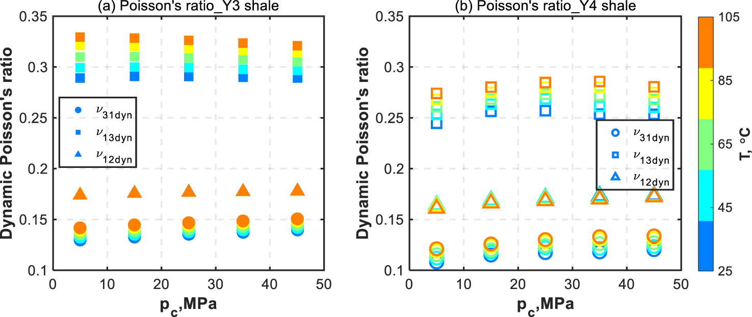
Three dynamic Poisson's ratios (ν31dyn, ν13dyn, ν12dyn) as functions of the confining pressure (pc) and temperature (T) for (a) #Y3 and (b) #Y4 shales.
Additionally, both ν31dyn and ν13dyn are positive functions of the applied temperature at any confining pressure condition. At 5 MPa confining pressure, ν31dyn increases by 9.2%, whereas ν13dyn increases by 13.9% over the entire temperature range for #Y3 shale, as shown in Figure 9a. The increasing degree of both Poisson’s ratios with temperature generally decreases with the increasing confining pressure. However, for #Y4 shale shown in Figure 9b, the increase of Poisson’s ratio with rising temperature reaches the maximum when the confining pressure is 35 MPa. In contrast to ν31dyn and ν13dyn, temperature almost has no effect on ν12dyn.
3.2 Static properties of anisotropic shales
Figure 10 shows evolutions of the apparent static Young’s moduli (E33stapparent, E11stapparent) with the confining pressure (pc) and temperature (T) for two pairs of shale samples. Overall, both E33stapparent and E11stapparent exhibit increasing trends with the increasing confining pressure at any temperature level. The increase of the apparent static Young’s modulus over the entire pressure range is somewhat dependent on the temperature magnitude. For #Y3 shale shown in Figure 10a, the average increase with pressure is 40.3% for E33st and 64.8% for E11stapparent. For #Y4 shale shown in Figure 10b, the average increase with pressure is 15.9% for E33st and 56.0% for E11stapparent. E11stapparent is more sensitive to the confining pressure than E33stapparent.
FIGURE 10

Two apparent static Young’s moduli (E33stapparent, E11stapparent) as functions of the confining pressure (pc) and temperature (T) for (a) #Y3 and (b) #Y4 shales.
At a specific confining pressure, both E33stapparent and E11stapparent increase with the rising temperature. The increase over the applied temperature range depends on the confining pressure magnitude. For #Y3 shale shown in Figure 10a, the average increase with temperature is 14.9% for E33stapparent and 11.5% for E11st. For #Y4 shale shown in Figure 10b, the average increase with temperature is 18.4% for E33stapparent and 9.4% for E11stapparent. E11stapparent is more sensitive to the rising temperature than E33stapparent. In addition, E11st is larger than E33st at any confining pressure or temperature condition. As a result, E11stapparent/E33stapparent can reach as high as 2.1 for #Y3 shale and 1.99 for #Y4 shale.
Figure 11 exhibits the evolution of the apparent static Poisson’s ratios (ν31stapparent, ν13stapparent) with the confining pressure (pc) and temperature (T) for #Y3 and #Y4 shales. For #Y3 shale shown in Figure 11a, ν13stapparent is systematically greater than ν31st at any confining pressure or temperature conditions, whereas ν13stapparent is smaller at lower temperature levels but larger at higher temperature levels than ν31stapparent for #Y4 shale shown in Figure 11b. Overall, with the increased confining pressure at any temperature levels, both ν31stapparent and ν13stapparent continuously increase or increase to a maximum, after which they slowly decrease. For the temperature dependence, both static Poisson’s ratios exhibit very small temperature dependence.
FIGURE 11

Two apparent static Poisson’s ratios (ν31stapparent, ν13stapparent) as functions of the confining pressure (pc) and temperature (T) for (a) #Y3 and (b) #Y4 shales.
4 Discussion
4.1 Combined effects of confining pressure and temperature
4.1.1 Confining pressure dependence
For a shale sample with a transversely isotropic structure, the increase of the confining pressure tends to preferentially close microcracks aligned in the bedding planes and make the compaction of adjacent thin beds better. As a result, dynamic properties (i.e., velocities, Young’s modulus, and Poisson’s ratio) exhibit more pressure sensitivity in the bedding-normal direction than in the bedding-parallel direction, as seen in Figures 7–9. These results are consistent with many previous works on different types of shales (Meléndez-Martínez and Schmitt, 2016). In addition, the dynamic properties of the selected shales are less sensitive to pressure than sandstones with similar porosity. For instance, the P-wave velocity increase is typically larger than 10% for sandstones (Han et al., 1986), whereas the increase is less than 7.0% at the temperature of 25 °C for the selected shales shown in Figure 7. For sandstones, the solid grain framework and pore structure dominate the pressure dependence of velocities (King, 1966; Mobarak and Somerton, 1971; Wang et al., 2020a), while in shales, the pressure dependence of velocities is closely related to the clay-supported framework, which is relatively unaffected by the confining pressure (Johnston, 1987).
However, from a static perspective, the effects of the increased confining pressure can be characterized by the ability to restrain the axial compaction and radial expansion. Given the weak cohesive strength of bedding planes and the preferred alignment of microcracks, the increased confining pressure is more prone to play an inhibitory role in the direction perpendicular to bedding planes when measuring horizontal samples. As a result, bedding-parallel static properties (E11stapparent, ν13stapparent) are more sensitive to the applied confining pressure than bedding-normal ones (E33stapparent, ν31stapparent), as seen in Figures 10, 11.
4.1.2 Temperature dependence
As shown in Table 1 and Figure 2, the selected shales are mixtures of solid grains, soft clays, and kerogen. With increased temperature, the rock material would thermally expand (Zhang et al., 2015; Herrmann et al., 2018; Ding et al., 2020). Thermal expansion coefficients of rock materials frequently vary with their mineralogical compositions. For example, the volumetric thermal expansion coefficients of quartz (Palciauskas and Domenico, 1982) and feldspar (Bass, 1995; Ghabezloo and Sulem, 2009) are 33.4 × 10⁻⁶ K−1 and 11.1 × 10⁻⁶ K−1, respectively. Different from the solid grain expansion, the soft clay has the risk of exhibiting thermal expansion or contraction behavior in the process of heating, which might be caused by the dehydration of clay-bound water (Li and Wong, 2017; White et al., 2017; Gabova et al., 2020). In addition, as an essential component of organic shales, the presence of kerogen might play a role in the temperature-dependent properties. From one aspect, the thermal expansion coefficient of kerogen (∼3.4 × 10⁻⁴ K−1, as denoted by Smith and Johnson (1976)) is more than two orders of magnitude larger than that of rock-forming minerals (Gabova et al., 2020). From the other aspect, kerogen would be converted to oil and gas when the temperature is high enough (∼350 °C, as denoted by Bai et al. (2017)). However, as in this study, phase changes of kerogen have no effects on the temperature-dependent properties, as the maximum temperature, 105 °C, is too low to decompose kerogen.
Another important characteristic of organic shales is the presence of thin bedding planes, which, in turn, would influence the temperature-dependent properties of shales. Gabova et al. (2020) measured the linear thermal expansion coefficient of organic-rich shales in both directions parallel and perpendicular to rock beddings within a temperature range from 25 °C to 300 °C. The conclusion is that higher thermal expansion coefficients can be found in the direction perpendicular to bedding planes for transversely isotropic shales. The unequal expansion in the orthogonal directions is expected to create thermal cracks in the preferred orientation parallel to bedding planes, as demonstrated by Zhou et al. (2016) using SEM images after the bedded sandstone is heated and damaged.
The anisotropic and distinct expansion behaviors of the shale components alter the internal structure of the rock mass in the process of heating, which further leads to changes in rock elastic or mechanical properties. From a dynamic perspective, porosity is the first-level influencing factor for the ultrasonic velocities. On the one hand, thermal expansion of solid grains causes grain rearrangement and crack propagation, increasing porosity (Hassanzadegan et al., 2014; Li and Wong, 2017; Gabova et al., 2020). On the other hand, solid grains and their contacts are thermally softened in the process of increasing temperature (Wang and Nur, 1988). Both factors contribute to the decrease in ultrasonic velocity with increasing temperature (Figure 7). Subsequently, the calculated dynamic Young’s moduli and Poisson’s ratio (see Figures 8, 9) demonstrate decreasing and increasing trends with the increasing temperature, respectively, if the bulk density changes in the process of heating are ignored. When mentioning the apparent static elastic properties, as shown in Figure 12, when applying an axial load to the rock sample, the static Young’s modulus is the ratio between the applied axial stress and the induced axial strain at room temperature. However, when the temperature increases, the rock will expand, which induces a thermal strain in the opposite direction of the compression. The servo-controlled system will maintain the axial stress at a constant value, but the recorded strain is the sum of strains induced by axial load and strains induced by thermal expansion. Thus, the static Young’s modulus is reduced compared with that at room temperature (Figure 10). In the radial direction, the radial strain induced by the axial load and the thermal strain induced by thermal expansion have the same direction. Thus, the apparent static Poisson’s ratio would increase with increasing temperature (Figure 11).
FIGURE 12

Schematic of the effects of temperature on static Young’s modulus.
4.1.3 Combined effects of confining pressure and temperature
When applying the above findings to practical interpretations, special care should be taken in considering the mechanical properties with the increasing burial depth. Figure 13 schematically exhibits the combined pressure and temperature effects on dynamic and static Young’s moduli, with the vertical axis as the schematic burial depth. It is pertinent to mention that this highlights the coupling effects of confining pressure and temperature as a function of depth, without considering other geological factors (e.g., porosity, organic matter, mineral composition) affecting the mechanical properties of organic shales.
FIGURE 13

Schematic of the coupling effects of confining pressure (pc) and temperature (T) on dynamic and static Young’s moduli of organic shales. Note: the vertical axis schematically indicates the burial depth.
First, increased confining pressure and temperature oppositely affect dynamic Young’s moduli, as shown in Figure 13. Although the two effects can offset each other to a certain degree over the applied temperature and confining pressure ranges, the temperature effect predominates. The same conclusion can be applied to the results of ultrasonic velocities shown in Figure 7, which is significant in estimating the reservoir properties. Effects of temperature appear to be too large to be ignored in estimating reservoir properties from acoustic logs. Mobarak and Somerton (1971) reported that ignoring the effects of temperature on acoustic velocities could result in an overestimation of porosity by nearly one-third. In addition, different from effects on velocities and Young’s moduli, increased pressure and temperature tend to increase the dynamic Poisson’s ratios shown in Figure 7 collectively. These could be attributed to the compaction effect from increased pressure and the softening effect from rising temperature.
Second, the effects of temperature on dynamic properties shown in Figures 7–9 are less pronounced at higher confining pressure. This finding for selected shales is consistent with results from many peer researchers (Timur, 1977) in sandstones. On the contrary, the effects of confining pressure on dynamic properties are increased at higher temperature levels. These can be attributed to the thermal softening of grain boundaries and the thermally induced cracks. At higher confining pressure, the generated cracks do not remain open to decrease temperature effects, whereas at a higher temperature, the thermal softening and induced cracks would enlarge the compressibility of rock materials.
Third, increased temperature and pressure affect static Young’s moduli shown in Figure 13 in the same manner, namely, increasing effects. In contrast, the increase of apparent static Young’s moduli contributed from increased confining pressure is systematically greater than that from increased temperature, regardless of the direction perpendicular or parallel to bedding planes. As shown in Figure 10, the increased confining pressure would increase temperature effects on static properties exactly as the rising temperature contributes to pressure effects. At lower confining pressure, thermal expansion of minerals would fill compliant pores or grain boundaries without increasing rock volume. However, at higher confining pressure, the compliant pores and boundaries are well compacted. The thermal expansion of minerals with temperature would increase rock volume, giving rise to a larger increase in the static Young’s modulus with temperature at higher confining pressure. Moreover, as shown in Figure 9, the increasing confining pressure generally increases the static Poisson’s ratio, whereas the rising temperature affects the apparent static Poisson’s ratio in a complex manner. At higher pressure, there exists a somewhat increasing trend of the static Poisson’s ratio with the rising temperature. However, overall, the temperature effect on the apparent static Poisson’s ratio is minor compared to the pressure effect.
4.2 Combined pressure-temperature effects on anisotropy evolution
We use E11/E33 and ν13/ν31 as indicators to investigate the evolution of anisotropy degrees for two pairs of shales with varied confining pressure and temperature, as shown in Figure 14. From a dynamic perspective, E11/E33 presents a generally decreasing trend with the increasing pressure, which denotes that E33dyn is more sensitive to the applied confining pressure than E11dyn. Dynamic ν13/ν31 exhibits the same value and trend as dynamic E11/E33 because E11/E33 equals ν13/ν31, which is always satisfied for the transverse isotropic medium within the regime of elasticity (Mavko et al., 2009; Wang et al., 2021b). However, from the static perspective, the applied confining pressure influences E11stapparent more than E33stapparent (Figure 13). As a result, static E11/E33 reveals an increasing trend with increasing confining pressure to approach the dynamic E11/E33 at the maximum confining pressure. A comparison shows that the static anisotropy indicator, E11/E33, is more sensitive to the confining pressure than the dynamic one. For the static ν13/ν31, there is a big jump when the temperature increases from 45 °C to 65 °C, as shown in Figures 14c,d. After carefully analyzing the evolution of static ν13/ν31 with confining pressure at temperatures of 65 °C, 85 °C, and 105 °C, the static ν13/ν31 generally displays a first increasing and then decreasing trend with the increased confining pressure for both samples.
FIGURE 14

Dynamic and static anisotropy degree, E11/E33, as functions of the confining pressure and temperature for (a) #Y3 and (b) #Y4 shales; ν13/ν31 as functions of the confining pressure and temperature for (c) #Y3 and (d) #Y4 shales.
For the temperature-dependent anisotropy evolutions, dynamic E11/E33 essentially increases with the rising temperature for the #Y3 shale shown in Figure 14a but nearly remains constant for #Y4 shale over the applied temperature range shown in Figure 14b. The different behaviors of the two shales might be attributed to the compositional differences and the internal heterogeneity. The increasing anisotropy degree for #Y3 shale can be explained by the more softening effects in the direction perpendicular to bedding planes in the process of heating. However, the static E11/E33 decreases to its minimum at 85 °C, after which it increases for #Y3 shale shown in Figure 14a, while the static E11/E33 presents an overall decreasing trend over the temperature range for #Y4 shale shown in Figure 14b. The anisotropic thermal expansion can easily explain these decreasing trends in transversely isotropic shales; that is, a higher thermal expansion coefficient can be found in the bedding-normal direction to increase E33stapparent with a greater magnitude. The subsequent increase of static E11/E33 when the temperature is increased from 85 °C to 105 °C in #Y3 shale might be caused by the internal heterogeneity. For static ν13/ν31 at temperatures of 65 °C, 85 °C, and 105 °C, the effect of increasing temperature on static ν13/ν31 is tiny.
Figures 14a,b show that increased confining pressure and temperature have opposite influences on the anisotropy evolution for the dynamic and static Young’s moduli. The increased confining pressure tends to close microcracks along bedding planes and compact more in the direction perpendicular to bedding planes, whereas the increased temperature attempts to create thermal cracks along bedding planes and expand more in the direction perpendicular to bedding planes. In contrast to the static E11/E33, the static ν13/ν31 at higher temperature levels (65 °C, 85 °C, and 105 °C) shown in Figures 14c,d is a weaker function of the confining pressure and temperature. This might be explained by the fact that the pressure compaction or thermal expansion affects axial and radial strains in the same manner, which can offset their effects on the static ν13/ν31.
4.3 Combined pressure-temperature effects on dynamic–static correlations
By comparing Figures 8–11, the dynamic Young’s modulus and Poisson’s ratio substantially exceed the static ones at varied confining pressure and temperature conditions. Difference in strain amplitude is frequently considered to be the major cause of the differences between dynamic and static elastic properties (Walsh, 1965; Tutuncu et al., 1998; Fjær, 2019; Wang et al., 2022). In addition, as stated by Fjær et al. (2013), the strain rate induced during the rock mechanical laboratory test corresponds to that induced by a passing elastic wave with a frequency of approximately 1 Hz, which is within the seismic frequency range. The dynamic and static elastic properties might be equal if dynamic moduli are derived from seismic velocities (Fjær, 2019). It is well established that dynamic elastic properties are frequency-dependent. The rock would behave in a stiffer manner under ultrasonic frequency than under seismic frequency (Batzle et al., 2006; Borgomano et al., 2019; Gallagher et al., 2022). Given that the dynamic properties are derived from ultrasonic velocities, the difference between dynamic and static elastic properties might be overestimated.
Due to uncertainties in measuring static Poisson’s ratios, Figure 15 only exhibits correlations between dynamic and static Young’s moduli over the applied confining pressure and temperature ranges, intending to uncover the coupled thermomechanical effects on dynamic–static property correlations. The size of the scatter shown in Figure 15 is scaled with respect to the confining pressure, with a bigger size representing a higher confining pressure. The maximum confining pressure and temperature in the measurements are, to some extent, to simulate the in situ effective horizontal stress and temperature subjected to a reservoir with 2–3 km burial depth. It is pertinent to mention that, given the limitations of the pseudo-triaxial testing system, the axial stress must be equal to or greater than the radial confining stress during laboratory measurements. When measuring a horizontal shale plug, the applied axial stress more closely represents the maximum horizontal stress, as is the case in a thrust fault. The uniform radial confining stress must represent both the vertical overburden stress and the minimum horizontal stress, which are far from equal in the field condition (Zoback et al., 2003; Barree et al., 2009). If the in situ stress state corresponds to the case of a normal fault, the radial stress normal to bedding when measuring a horizontal shale plug is far less than the vertical overburden stress. As a result, it is impossible to precisely simulate the in situ stress for a horizontal shale sample.
FIGURE 15

Dynamic and static Young’s modulus correlations over the applied pressure and temperature ranges for (a) #Y3 and (b) #Y4 shales. The size of the scatters represents the pressure magnitude, with larger scatters indicating higher pressures.
As shown in Figure 15, the increased pressure increases both dynamic and static Young’s moduli, with larger increases for the static Young’s modulus. If the effects of confining pressure are ignored, the dynamic–static correlation coefficient in the bedding-normal direction (E33) would be overestimated by 28.9% for #Y3 shale and 6.2% for #Y4 shale, whereas an overestimation of more than 50% for the dynamic–static correlation coefficient in the bedding-parallel direction (E11) would result. Additionally, the rising temperature has opposite effects on dynamic and static properties by decreasing dynamic moduli and increasing static moduli. Ignoring the temperature effect would induce a general overestimation of the dynamic–static correlation coefficient by approximately 35% for E33 and about 25% for E11. More importantly, with the combined effects of pressure and temperature, the dynamic–static correlation coefficient would move from 5:2 (close to surface conditions) to 3:2 (close to in situ conditions) for E33 and move from 7:2 to 3:2 for E11.
4.4 Implications and limitations
It is acknowledged that differences between dynamic and static elastic parameters exist (Fjær, 2019). Establishing an accurate dynamic-to-static transformation model is critical for many geoengineering applications. However, with respect to the dynamic–static elasticity mismatch, most previous investigations focus on the effects of stress/pressure (Sone and Zoback, 2013; Ong et al., 2016; Ramos et al., 2019; Wang et al., 2021a; Han et al., 2021; Wang et al., 2025). Little research investigates the temperature effects on the dynamic–static mechanical relationships, let alone the combined pressure-temperature effects. To reveal the mechanism for dynamic–static elasticity differences under in situ conditions, we innovatively provide an experimental procedure to jointly evaluate temperature-pressure effects on dynamic–static relationships in anisotropic shales. The findings have significant implications for many geo-applications, like reservoir evaluation, hydraulic fracturing design, and stimulation strategies. The law of “convergence of dynamic and static modulus anisotropy at high pressure and divergence at high temperature” revealed by the experimental data provides a valuable in situ parameter correction benchmark for cross-scale geoengineering modeling and effective reservoir stimulation.
It should be noted that such laboratory-scale findings still have limitations in direct field applications. First, the cylindrical samples have limitations in capturing the cross-scale heterogeneity in the real shale formations, potentially failing in reflecting the field-scale dynamic and static properties. Second, the pseudo-triaxial rock mechanics testing system used in the current study is restricted to obtaining the full stiffness tensor for transversely isotropic shales, especially the parameter of c13. The use of inferred c13 from empirical relations might create potential errors in calculating dynamic Young’s modulus and Poisson’s ratio. Third, other in situ factors, like pore fluids, organic matter maturity, and mineralogical variations, are less considered due to the limited sample amounts. This might create limitations in fully reflecting the in situ conditions. Nevertheless, the dynamic–static elasticity gap and the corresponding mechanism revealed in this study remain meaningful for geoengineering interpretations. The focus of future work will be on enhancing the applicability in cross-scale geoengineering evaluation by establishing robust dynamic–static correlations approaching real in situ conditions.
5 Conclusion
In this study, we perform a suite of triaxial tests on two pairs of organic shales with transversely isotropic texture to explore the combined effects of confining pressure and temperature on mechanical properties from both dynamic and static aspects. The experiments are conducted at varied temperatures from 25 °C to 105 °C and confining pressures from 5 MPa to 45 MPa. Through analyzing the laboratory data, we draw the following conclusions.
An increase in confining pressure and temperature affects dynamic Young’s moduli in an opposite manner by showing increasing and decreasing trends, respectively, but jointly increases the apparent static Young’s modulus. The dynamic Poisson’s ratio increases with the increasing confining pressure and temperature, whereas the apparent static Poisson’s ratio exhibits non-uniform relations to pressure and temperature. A temperature increment increases pressure effects on both dynamic and static properties, while the confining pressure increment weakens temperature effects on dynamic properties but increases temperature effects on static properties.
Dynamic and static Young’s modulus anisotropy (E11/E33) evolutions are oppositely affected by the increased confining pressure and temperature, which can be attributed to the fact that both pressure compaction and thermal expansion are anisotropic due to the existence of bedding planes. With the increasing confining pressure, dynamic and static E11/E33 tend to approach each other at the maximum confining pressure, whereas dynamic and static E11/E33 tend to diverge from each other with the rising temperature.
Over the applied confining pressure and temperature ranges, the dynamic Young’s modulus and Poisson’s ratio are systematically greater than the static ones. However, the correlation coefficients between dynamic and static Young’s modulus are largely influenced by the varied confining pressure and temperature conditions. Ignoring either effect would result in an overestimation of the dynamic–static Young’s modulus correlation coefficient.
Statements
Data availability statement
The raw data supporting the conclusions of this article will be made available by the authors, without undue reservation.
Author contributions
LH: Conceptualization, Investigation, Supervision, Writing – original draft, Writing – review and editing. XD: Investigation, Methodology, Writing – original draft. XW: Data curation, Formal Analysis, Validation, Writing – review and editing. YW: Formal Analysis, Investigation, Methodology, Writing – original draft.
Funding
The author(s) declare that financial support was received for the research and/or publication of this article. This work was supported by the National Natural Science Foundation of China (grant no. 42430810) and the SINOPEC Key Laboratory of Geophysics.
Conflict of interest
Authors LH, XD, and XW were employed by SINOPEC Geophysical Corporation. Author YW was employed by SINOPEC Geophysical Research Institute and SINOPEC Zhongyuan Oilfield Company.
The authors declare that this study received funding from SINOPEC Key Laboratory of Geophysics. The funder had the following involvement in the study: experiment design, data collection, and data interpretation.
Generative AI statement
The author(s) declare that no Generative AI was used in the creation of this manuscript.
Any alternative text (alt text) provided alongside figures in this article has been generated by Frontiers with the support of artificial intelligence and reasonable efforts have been made to ensure accuracy, including review by the authors wherever possible. If you identify any issues, please contact us.
Publisher’s note
All claims expressed in this article are solely those of the authors and do not necessarily represent those of their affiliated organizations, or those of the publisher, the editors and the reviewers. Any product that may be evaluated in this article, or claim that may be made by its manufacturer, is not guaranteed or endorsed by the publisher.
References
1
Arif M. Lebedev M. Barifcani A. Iglauer S. (2017). Influence of shale-total organic content on CO2 geo-storage potential. Geophys. Res. Lett.44 (17), 8769–8775. 10.1002/2017GL073532
2
Asef M. R. Najibi A. R. (2013). The effect of confining pressure on elastic wave velocities and dynamic to static Young’s modulus ratio. Geophysics78 (3), D135–D142. 10.1190/geo2012-0279.1
3
Bai F. Sun Y. Liu Y. Guo M. (2017). Evaluation of the porous structure of Huadian oil shale during pyrolysis using multiple approaches. Fuel187, 1–8. 10.1016/j.fuel.2016.09.012
4
Barree R. D. Gilbert J. V. Conway M. W. (2009). Stress and rock property profiling for unconventional reservoir stimulation. In: Society of Petroleum Engineers–SPE Hydraulic Fracturing Technology Conference; 2009 January 19–21; The Woodlands, Texas. p. 9–26.
5
Bass J. D. (1995). Elasticity of minerals, glasses, and melts. In: ThomasJ. A., editor. Mineral physics and crystallography: a handbook of physical constants. Washington, DC: American Geophysical Union Online Reference Shelf, Vol. 2. p. 45–63. 10.1029/rf002p0045
6
Batzle M. L. Han D. H. Hofmann R. (2006). Fluid mobility and frequency-dependent seismic velocity-direct measurements. Geophysics71 (1), N1–N9. 10.1190/1.2159053
7
Blake O. O. Faulkner D. R. (2016). The effect of fracture density and stress state on the static and dynamic bulk moduli of westerly granite. J. Geophys. Res. Sol. Ea.121 (4), 2382–2399. 10.1002/2015JB012310
8
Blake O. O. Ramsook R. Faulkner D. R. Iyare U. C. (2020). The effect of effective pressure on the relationship between static and dynamic Young’s moduli and Poisson’s ratio of naparima hill formation mudstones. Rock Mech. Rock Eng.53, 3761–3778. 10.1007/s00603-020-02140-0
9
Borgomano J. V. M. Pimienta L. X. Fortin J. Guéguen Y. (2019). Seismic dispersion and attenuation in fluid-saturated carbonate rocks: effect of microstructure and pressure. J. Geophys. Res. Sol. Ea.124 (12), 12498–12522. 10.1029/2019JB018434
10
Castelletto N. Gambolati G. Teatini P. (2013). Geological CO2 sequestration in multi-compartment reservoirs: geomechanical challenges. J. Geophys. Res. Sol. Ea.118 (5), 2417–2428. 10.1002/jgrb.50180
11
Chichinina T. Vernik L. (2018). Physical bounds on c13 and δ for organic mudrocks. Geophysics83 (5), A75–A79. 10.1190/geo2018-0035.1
12
Crisci E. Ferrari A. Laloui L. Schuster V. Rybacki E. Bonnelye A. et al (2022). Discussion on “Experimental Deformation of Opalinus Clay at Elevated Temperature and Pressure Conditions: mechanical Properties and the Influence of Rock Fabric” of Schuster, V., Rybacki, E., Bonnelye, A., Herrmann, J., schleicher, A.M., Dresen, G. Rock Mech. Rock Eng.55, 463–465. 10.1007/S00603-021-02654-1
13
Dewhurst D. N. Siggins A. F. (2006). Impact of fabric, microcracks and stress field on shale anisotropy. Geophys. J. Int.165 (1), 135–148. 10.1111/j.1365-246X.2006.02834.x
14
Ding C. Hu D. Zhou H. Lu J. Lv T. (2020). Investigations of P-Wave velocity, mechanical behavior and thermal properties of anisotropic slate. Int. J. Rock Mech. Min.127, 104176. 10.1016/j.ijrmms.2019.104176
15
Ewy R. T. (2018). Practical approaches for addressing shale testing challenges associated with permeability, capillarity and brine interactions. Geomech. Energy Envir.14, 3–15. 10.1016/J.GETE.2018.01.001
16
Fjær E. (2019). Relations between static and dynamic moduli of sedimentary rocks. Geophys. Prospect.67 (1), 128–139. 10.1111/1365-2478.12711
17
Fjær E. Stroisz A. M. Holt R. M. (2013). Elastic dispersion derived from a combination of static and dynamic measurements. Rock Mech. Rock Eng.46, 611–618. 10.1007/s00603-013-0385-8
18
Gabova A. Chekhonin E. Popov Y. Savelev E. Romushkevich R. Popov E. et al (2020). Experimental investigation of thermal expansion of organic-rich shales. Int. J. Rock Mech. Min.132, 104398. 10.1016/j.ijrmms.2020.104398
19
Gallagher A. Fortin J. Borgomano J. (2022). Seismic dispersion and attenuation in fractured fluid-saturated porous rocks: an experimental study with an analytic and computational comparison. Rock Mech. Rock Eng.55 (1-2), 4423–4440. 10.1007/s00603-022-02875-y
20
Ghabezloo S. Sulem J. (2009). Stress dependent thermal pressurization of a fluid-saturated rock. Rock Mech. Rock Eng.42 (1), 1–24. 10.1007/s00603-008-0165-z
21
Gong F. Di B. Wei J. Ding P. Tian H. Han J. (2019). A study of the anisotropic static and dynamic elastic properties of transversely isotropic rocks. Geophysics84 (6), C281–C293. 10.1190/geo2018-0590.1
22
Han D. H. Nur A. Morgan D. (1986). Effects of porosity and clay content on wave velocities in sandstones. Geophysics51 (11), 2093–2107. 10.1190/1.1442062
23
Han T. Yu H. Fu L. Y. (2021). Correlations between the static and anisotropic dynamic elastic properties of lacustrine shales under triaxial stress: examples from the Ordos Basin, China. Geophysics86 (4), MR191–MR202. 10.1190/geo2020-0761.1
24
Hassanzadegan A. Blöcher G. Zimmermann G. Milsch H. (2012). Thermoporoelastic properties of flechtinger sandstone. Int. J. Rock Mech. Min.49, 94–104. 10.1016/j.ijrmms.2011.11.002
25
Hassanzadegan A. Blöcher G. Milsch H. Urpi L. Zimmermann G. (2014). The effects of temperature and pressure on the porosity evolution of flechtinger sandstone. Rock Mech. Rock Eng.47 (2), 421–434. 10.1007/s00603-013-0401-z
26
Herrmann J. Rybacki E. Sone H. Dresen G. (2018). Deformation experiments on bowland and posidonia shale—part I: strength and Young’s modulus at ambient and in situ pc-T conditions. Rock Mech. Rock Eng.51 (12), 3645–3666. 10.1007/s00603-018-1572-4
27
ISRM (2007). The complete ISRM suggested methods for rock characterization, testing and monitoring: 1974–2006. In: UlusayR.HudsonJ. A., editors. Suggested methods prepared by the commission on testing methods. Ankara: International Society for Rock Mechanics, Compilation Arranged by the ISRM Turkish National Group.
28
Johnston D. H. (1987). Physical properties of shale at temperature and pressure. Geophysics52 (10), 1391–1401. 10.1190/1.1442251
29
Johnston J. E. Christensen N. I. (1995). Seismic anisotropy of shales. J. Geophys. Res.100, 5991–6003. 10.1029/95JB00031
30
Jones T. Nur A. (1983). Velocity and attenuation in sandstone at elevated temperatures and pressures. Geophys. Res. Lett.10 (2), 140–143. 10.1029/gl010i002p00140
31
Kern H. (1978). The effect of high temperature and high confining pressure on compressional wave velocities in quartz-bearing and quartz-free igneous and metamorphic rocks. Tectonophysics44 (1-4), 185–203. 10.1016/0040-1951(78)90070-7
32
King M. S. (1966). Wave velocities in rocks as a function of changes in overburden pressure and pore fluid saturants. Geophysics31 (1), 50–73. 10.1190/1.1439763
33
Kiuru R. Nieman P. Rinne M. (2023). Evaluation of the performance of the ISRM suggested methods for measuring density and porosity when applied to low-porosity rocks. IOP Conf. Ser. Earth Environ. Sci.1124, 012020. 10.1088/1755-1315/1124/1/012020
34
Kovari K. Tisa A. Einstein H. H. Franklin J. A. (1983). Suggested methods for determining the strength of rock materials in triaxial compression: revised version. Int. J. Rock Mech. Min. and Geomech. Abs.20 (6), 285–290. 10.1016/0148-9062(83)90598-3
35
Li Y. Schmitt D. R. (1998). Drilling-induced core fractures and in situ stress. J. Geophys. Res. Sol. Ea.103 (B3), 5225–5239. 10.1029/97JB02333
36
Li B. Wong R. C. K. (2017). Modeling anisotropic static elastic properties of soft mudrocks with different clay fractions. Geophysics82 (1), MR27–MR37. 10.1190/geo2015-0575.1
37
Lo T. W. Coyner K. B. Toksöz M. N. (1986). Experimental determination of elastic anisotropy of Berea sandstone, chicopee shale, and Chelmsford granite. Geophysics51, 164–171. 10.1190/1.1442029
38
Masri M. Sibai M. Shao J. F. Mainguy M. (2014). Experimental investigation of the effect of temperature on the mechanical behavior of tournemire shale. Int. J. Rock Mech. Min.70, 185–191. 10.1016/j.ijrmms.2014.05.007
39
Mavko G. Mukerji T. Dovorkin J. (2009). The rock physics handbook - tools for seismic analysis of porous media. Cambridge: Cambridge University Press. 2nd Edition.
40
Meléndez-Martínez J. Schmitt D. R. (2016). A comparative study of the anisotropic dynamic and static elastic moduli of unconventional reservoir shales: implication for geomechanical investigations. Geophysics81 (3), D245–D261. 10.1190/geo2015-0427.1
41
Mobarak S. A. Somerton W. H. (1971). The effect of temperature and pressure on wave velocities in porous rocks. In: Society of petroleum engineers–fall meeting of the society of petroleum engineers of AIME; October 3–6, 1971; New Orleans, Louisiana: OnePetro. 10.2118/3571-MS
42
Niandou H. Shao J. F. Henry J. P. Fourmaintraux D. (1997). Laboratory investigation of the mechanical behaviour of tournemire shale. Int. J. Rock Mech. Min.34 (1), 3–16. 10.1016/s0148-9062(96)00053-8
43
Ong O. N. Schmitt D. R. Kofman R. S. Haug K. (2016). Static and dynamic pressure sensitivity anisotropy of a calcareous shale. Geophys. Prospect.64 (4), 875–897. 10.1111/1365-2478.12403
44
Palciauskas V. V. Domenico P. A. (1982). Characterization of drained and undrained response of thermally loaded repository rocks. Water Resour. Res.18 (2), 281–290. 10.1029/WR018i002p00281
45
Ramos M. J. Espinoza D. N. Laubach S. E. Torres-Verdín C. (2019). Quantifying static and dynamic stiffness anisotropy and nonlinearity in finely laminated shales: experimental measurement and modeling. Geophysics84 (1), MR25–MR36. 10.1190/geo2018-0032.1
46
Ren J. Wang Y. Han D. H. Zhao L. Long T. Tang S. (2021). Determining crack initiation stress in unconventional shales based on strain energy evolution. J. Geophys. Eng.18 (5), 642–652. 10.1093/jge/gxab041
47
Schuster V. Rybacki E. Bonnelye A. Herrmann J. Schleicher A. M. Dresen G. (2021). Experimental deformation of opalinus clay at elevated temperature and pressure conditions: mechanical properties and the infuence of rock fabric. Rock Mech. Rock Eng.54, 4009–4039. 10.1007/s00603-021-02675-w
48
Smith J. W. Johnson D. R. (1976). Mechanisms helping to heat oil-shale blocks. Am. Chem. Soc. Div. Fuel Chem.21 (6).
49
Somerton W. H. (1992). Thermal properties and temperature-related behavior of rock/fluid systems. Amsterdam, Netherlands: Elsevier.
50
Sone H. Zoback M. D. (2013). Mechanical properties of shale-gas reservoir rocks - part 1: static and dynamic elastic properties and anisotropy. Geophysics78 (5), D381–D392. 10.1190/geo2013-0050.1
51
Thomsen L. (1986). Weak elastic anisotropy. Geophysics51 (10), 1954–1966. 10.1190/1.1442051
52
Timur A. (1977). Temperature dependence of compressional and shear wave velocities in rocks. Geophysics42 (5), 950–956. 10.1190/1.1440774
53
Tutuncu A. N. Podio A. L. Gregory A. R. Sharma M. M. (1998). Nonlinear viscoelastic behavior of sedimentary rocks, part I: effect of frequency and strain amplitude. Geophysics63 (1), 184–194. 10.1190/1.1444311
54
Vernik L. (2016). Seismic petrophysics in quantitative interpretation. Houston, Texas: Society of Exploration Geophysicists.
55
Vernik L. Nur A. (1992). Ultrasonic velocity and anisotropy of hydrocarbon source rocks. Geophysics57 (5), 727–735. 10.1190/1.1443286
56
Walsh J. B. (1965). The effect of cracks on the uniaxial elastic compression of rocks. J. Geophys. Res.70 (2), 399–411. 10.1029/JZ070i002p00399
57
Wang Z. (2002). Seismic anisotropy in sedimentary rocks - part 2: laboratory data. Geophysics67 (5), 1423–1440. 10.1190/1.1512743
58
Wang Z. Nur A. (1988). Effect of temperature on wave velocities in sands and sandstones with heavy hydrocarbons. SPE Res. Eng.3 (1), 158–164. 10.2118/15646-PA
59
Wang Y. Han D. H. Li H. Zhao L. Ren J. Zhang Y. (2020a). A comparative study of the stress-dependence of dynamic and static moduli for sandstones. Geophysics85 (4), MR179–MR190. 10.1190/geo2019-0335.1
60
Wang Y. Zhao L. Han D. H. Qin X. Ren J. Wei Q. (2020b). Micro-mechanical analysis of the effects of stress cycles on the dynamic and static mechanical properties of sandstone. Int. J. Rock Mech. Min.134 (1), 104431. 10.1016/j.ijrmms.2020.104431
61
Wang Y. Zhao L. Han D. H. Mitra A. Li H. Aldin S. (2021a). Anisotropic dynamic and static mechanical properties of organic-rich shale: the influence of stress. Geophysics86 (2), C51–C63. 10.1190/geo2020-0010.1
62
Wang Y. Long T. Zhao L. Zhang Y. Han D. H. (2021b). Coupling effects of pressure and temperature on mechanical properties of organic shale. SEG-Society Explor. Geophys.2021 (1-IMAGE21), 2313–2317. 10.1190/segam2021-3580826.1
63
Wang Y. Zhao L. Han D. H. Wei Q. Zhang Y. Yuan H. et al (2022). Experimental quantification of the evolution of the static mechanical properties of tight sedimentary rocks during increasing-amplitude load and unload cycling. Geophysics87 (2), MR73–MR83. 10.1190/geo2021-0232.1
64
Wang Y. Zhao L. Yan D. Ma L. Cai Z. Zhu B. et al (2025). Anisotropic dynamic-static elasticity correlations in lacustrine shales: experimental insights for in situ stress estimation. Int. J. Rock Mech. Min.193, 106182. 10.1016/j.ijrmms.2025.106182
65
White J. A. Burnham A. K. Camp D. W. (2017). A thermoplasticity model for oil shale. Rock Mech. Rock Eng.50 (3), 677–688. 10.1007/s00603-016-0947-7
66
Yan F. Vernik L. Han D. H. (2019). Relationships between the anisotropy parameters for transversely isotropic mudrocks. Geophysics84 (6), MR195–MR203. 10.1190/geo2019-0088.1
67
Zhang P. Mishra B. Heasley K. A. (2015). Experimental investigation on the influence of high pressure and high temperature on the mechanical properties of deep reservoir rocks. Rock Mech. Rock Eng.48 (6), 2197–2211. 10.1007/s00603-015-0718-x
68
Zhao L. Qin X. Han D. H. Geng J. Yang Z. Cao H. (2016). Rock-physics modeling for the elastic properties of organic shale at different maturity stages. Geophysics81 (5), D527–D541. 10.1190/geo2015-0713.1
69
Zhou H. Liu H. Hu D. Yang F. Lu J. Zhang F. (2016). Anisotropies in mechanical behaviour, thermal expansion and P-Wave velocity of sandstone with bedding planes. Rock Mech. Rock Eng.49, 4497–4504. 10.1007/s00603-016-1016-y
70
Zoback M. D. Barton C. A. Brudy M. Castillo D. A. Finkbeiner T. Grollimund B. R. et al (2003). Determination of stress orientation and magnitude in deep wells. Int. J. Rock Mech. Min.40 (7-8), 1049–1076. 10.1016/j.ijrmms.2003.07.001
Summary
Keywords
anisotropic shales, in situ property, Young’s modulus, Poisson’s ratio, dynamic-static correlation
Citation
Hu L, Dong X, Wang X and Wang Y (2025) Static and dynamic mechanical responses of organic shales under combined temperature and confining pressure conditions. Front. Earth Sci. 13:1671172. doi: 10.3389/feart.2025.1671172
Received
22 July 2025
Revised
28 September 2025
Accepted
14 October 2025
Published
13 November 2025
Volume
13 - 2025
Edited by
Juntao Liu, Lanzhou University, China
Reviewed by
Lei Gao, Hohai University, China
Weichen Zhan, The University of Texas at Austin, United States
Updates
Copyright
© 2025 Hu, Dong, Wang and Wang.
This is an open-access article distributed under the terms of the Creative Commons Attribution License (CC BY). The use, distribution or reproduction in other forums is permitted, provided the original author(s) and the copyright owner(s) are credited and that the original publication in this journal is cited, in accordance with accepted academic practice. No use, distribution or reproduction is permitted which does not comply with these terms.
*Correspondence: Yang Wang, ywang0630@hotmail.com
Disclaimer
All claims expressed in this article are solely those of the authors and do not necessarily represent those of their affiliated organizations, or those of the publisher, the editors and the reviewers. Any product that may be evaluated in this article or claim that may be made by its manufacturer is not guaranteed or endorsed by the publisher.