Methods for seismic sedimentology and inversion using physics-driven convolutional model-based artificial intelligence

Seismic inversion is vital for reservoir characterization but faces significant challenges in complex fluvial-deltaic systems due to strong heterogeneity and thin-bedded formations. Current methods, including convolution-based, geostatistical, and artificial neural network (ANN) approaches, are often limited by wavelet stationarity assumptions, spatial uncertainty, and physical implausibility. This study develops a novel artificial intelligence (AI) seismic inversion algorithm that integrates a convolutional physical model with data-driven learning to overcome these drawbacks. The proposed physics-guided hybrid model employs a multi-wavelet inversion framework, incorporating 8–10 spatially variable wavelets per inversion cell to account for lateral wavelet variability. These physically constrained inversion candidates are then intelligently fused using a computationally efficient neural network, which maintains a 3.4% training error and 4.7% validation accuracy. This integrated approach achieves remarkable improvements: a 30% enhancement in vertical resolution enabling 1–3m thin-bed detection, a 40% improvement in lateral continuity (with correlation coefficients increasing from <0.6 to >0.85), and 70% better noise suppression. Application in a complex fluvial-deltaic system covering 7.2 km² with 80 wells confirmed the method’s robustness, delivering over 80% accuracy in sandbody prediction while significantly reducing geologically implausible results.

1 Introduction

Seismic inversion is a cornerstone of hydrocarbon exploration, transforming seismic reflection data into quantitative subsurface properties like acoustic impedance (El-Sayed et al., 2025; Zrelli et al., 2023). However, accurately characterizing complex fluvial-deltaic systems, noted for their intricate architectures, strong heterogeneity, and rapidly varying facies, remains a significant challenge for conventional inversion techniques (Sun et al., 2021; Liu et al., 2024; Bao et al., 2025).

Current mainstream methods each possess critical limitations in this context. Convolution-based inversion typically relies on a stationary wavelet, an assumption that is frequently violated in practice. Ignoring the spatial variability of wavelet amplitude, phase, and frequency leads to inaccurate reflectivity estimates, limits vertical resolution, and obscures thin-bed detection (Genovese and Palmeri, 2025; Dong et al., 2022; Hui et al., 2024).

To enhance resolution, geostatistical inversion incorporates spatial statistics from well data. However, in complex continental settings with rapid lateral changes, the fundamental assumption of spatial stationarity is often invalid (Mao et al., 2024; Zhang et al., 2022; Cabrera-Navarrete et al., 2020). The method becomes highly sensitive to limited well control, leading to non-unique solutions and geologically implausible sand-body geometries that fail to capture true depositional patterns (Abuzaied et al., 2023; Zhang et al., 2021). As shown in Figure 1, variograms computed in the east-west and north-south directions exhibit marked anisotropy, reflecting directional disparities in sediment distribution that standard geostatistical tools fail to adequately capture (Zhang et al., 2021; Liu et al., 2019).

Figure 1

Figure 1. Variograms in east-west and north-south directions. (a) Variograms EW (b) Variograms NS.

More recently, Artificial Neural Network (ANN)-based inversion has shown promise in learning complex, non-linear relationships from data (Hui et al., 2021; Yao et al., 2025; Hui et al., 2023a). While offering advantages in computational speed and automatic feature extraction, purely data-driven ANNs are often hampered by the “black-box” problem, poor generalization when well data is scarce, and a tendency to produce physically implausible results if not properly constrained (Li et al., 2019; Zhang et al., 2018; Fabien-Ouellet, 2020). Their performance is also heavily dependent on large volumes of high-quality training data (Su et al., 2023a; Hui et al., 2022).

The shortcomings of these methods—specifically, the physical oversimplification of convolution methods, the statistical instability of geostatistical approaches in heterogeneous environments, and the limited interpretability and physical consistency of pure AI models—collectively highlight a critical need for a more robust framework (Baddari et al., 2009; Pi et al., 2025; Chen et al., 2023). These shortcomings include distorted sand body shapes, fragmented connectivity, and incorrect spatial relationships. Figure 2 exemplifies these issues, where the simulated sand distributions deviate significantly from expected depositional patterns, reducing their geological reliability and practical value (Zhao and Chen, 2023). An ideal solution would integrate the principled constraints of physics-based modeling with the adaptive power of artificial intelligence. In fluvial–deltaic settings, conventional post-stack or geostatistical inversions often exhibit blurred sand–shale boundaries and limited lateral continuity, especially where wavelet non-stationarity and thin interbeds prevail. Recent studies further show challenges in capturing channel–lobe transitions and realistic geometry (Harishidayat et al., 2015; Mahgoub et al., 2017; Harishidayat et al., 2024; Jacobsen et al., 2025). These limitations motivate our physics-guided, multi-wavelet fusion strategy aimed at enhancing vertical resolution and inter-well continuity.

Figure 2

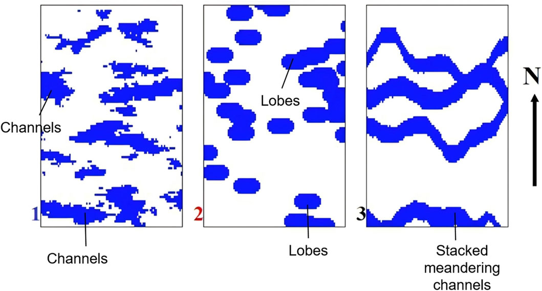
Figure 2. Simulated spatial distribution based on different variogram models.

Recent research in geotechnical modeling offers valuable insights that align with our study. Studies on the diffusion evolution rules of grouting slurry in mining-induced cracks and the disaster-causing mechanism of spalling rock bursts highlight the importance of diffusion models and geological failure mechanisms in understanding subsurface behavior (Cao et al., 2025a; Cao et al., 2025b). These studies inform the integration of such mechanisms into seismic inversion workflows, helping to improve inversion accuracy and geological consistency in complex sedimentary systems.

To address this gap, we propose a convolutional physical model-driven AI inversion method. This hybrid approach is innovatively designed to overcome the above limitations by leveraging a multi-wavelet inversion scheme to generate physically-grounded candidate solutions, which are then intelligently fused by a streamlined neural network. This methodology directly tackles the issues of wavelet non-stationarity, enhances vertical resolution and lateral continuity, and ensures the results are both geologically interpretable and computationally efficient. This study details the development of this method and demonstrates its superior performance in a complex fluvial-deltaic reservoir.

2 Methodology

2.1 Field background and datasets

The study area is located in the Gaotaizi region of the Daqing Oilfield, China, characterized by fluvial-deltaic sedimentary facies developed under continental settings. Channel sands typically show bell-shaped GR motifs and high-impedance seismic responses, whereas deltaic lobes display coarsening-upward GR with moderate impedance contrasts. Figure 3 shows the of wells used for AI-assisted inversion in this work. The available data consist of acoustic logs (AC), density logs, formation tops, sandstone markers, and a full-stack seismic volume. The seismic data have a vertical resolution of approximately 40HZ (≈20 m) and a horizontal sampling of about 25 m in the target interval. Both seismic and logging data are used for well-to-seismic calibration.

Figure 3

Figure 3. The distribution of wells used for AI-assisted inversion. The basemap is the elevation of the studied area. The magenta line represents the well profile of Figure 10b.

The inversion inputs include seismic traces adjacent to wells, well log curves (e.g., SY_AC), wavelets extracted near each well, and spatial coordinate. The target output is an estimated log curve generated by the inversion.

Before inversion, standard data preprocessing is conducted to ensure consistency. This includes normalization of log data, alignment of sampling intervals, and depth matching between seismic and logging data. These steps provide a consistent input dataset for calculating reflection coefficients, extracting wavelets, and training the inversion model.

A total of 80 wells were used for inversion and interpretation, among which 10 representative wells are displayed in Figure 3 to show their spatial distribution across the fluvial–deltaic system.

2.2 Overview and technical workflow

This study presents a convolutional physics-guided AI inversion method that integrates multi-wavelet inversion with AI-based fusion. The method enhances seismic inversion by addressing wavelet non-stationarity and spatial heterogeneity in complex continental reservoirs. The overall workflow consists of two phases: model training and model application, as illustrated schematically in Figure 4 (Dwivedi et al., 2021; Hui et al., 2025).

1. Core Challenge in Convolution-Based Inversion. Conventional inversion methods often rely on either fixed or interpolated wavelets, both of which have clear limitations. Fixed wavelets ignore lateral variations in wavelet characteristics, leading to inversion results that fail to reflect subsurface heterogeneity. Interpolated wavelets, though spatially adjusted, lack physical grounding and often yield unstable outputs that are sensitive to wavelet selection, reducing reliability in practical applications.

2. Multi-Wavelet Inversion. To address this, the proposed method performs multiple convolution-based inversions for each seismic trace using wavelets extracted from adjacent wells. This results in a set of alternative reflection coefficient series for each trace. These outputs form a training dataset that incorporates spatial wavelet variability and serves as a set of physically informed priors for the subsequent AI learning step. The overall concept is illustrated in Figure 4.

3. AI-Based Fitting. The multiple inversion results are fused using a neural network, which optimizes the inversion output by leveraging its ability to map complex, non-linear relationships. This fusion step improves accuracy and continuity, while retaining consistency with both seismic data and physical constraints.

Figure 4

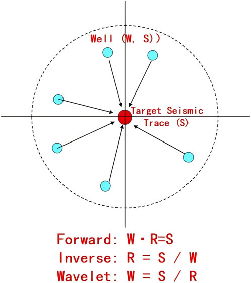
Figure 4. Schematic diagram of the convolutional physics-guided AI inversion workflow, illustrating the combination of spatially varying wavelets, multiple inversion candidates, and final AI-based fusion. The blue circle indicates the studied well and the red one in the middle represents the target seismic trace.

The detailed implementation is shown in Figure 5. During the model training phase, wavelets are first extracted from well data, and multi-wavelet inversion is performed on seismic traces adjacent to each well. The resulting candidate inversion curves, along with original well logs, are used to train the AI model. In the application phase, for any target trace, wavelets from surrounding wells are again used to generate multiple inversion candidates, which are fused by the trained model into a single, high-fidelity inversion output. This process is repeated across the seismic survey area to construct the final AI-assisted inversion volume (Dwivedi et al., 2021; Hui et al., 2023b).

Figure 5

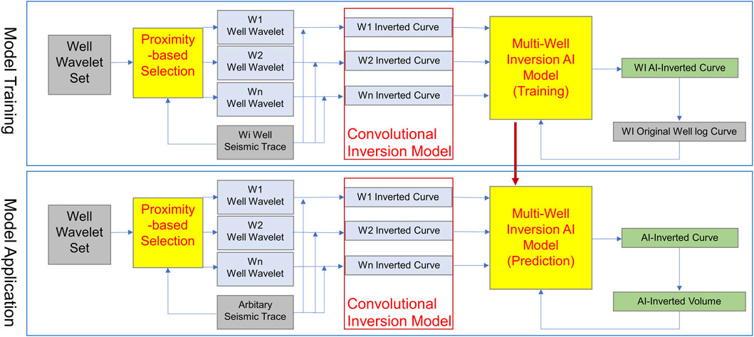
Figure 5. Workflow of the convolutional inversion and AI-assisted multi-well inversion process. Yellow boxes: model training phase. Green boxes: input and output features. Rey boxes: CNN architecture components. Light-blue boxes: inference or application phase. Red words: training variables or targets. Blue words: spatial parameters. Red rectangles: optimization modules.

2.3 Model architecture

The AI model used in this study is a hybrid convolutional neural network (CNN)-based architecture that integrates convolutional physical models with data-driven learning. The model architecture is designed to combine the strengths of deterministic physical modeling (wavelet-based convolutional inversion) with the flexibility and adaptive power of machine learning (neural network fitting). Below is a detailed breakdown of the architecture and training procedure.

2.3.1 Convolutional neural network (CNN) architecture

The CNN consists of the following main components.

2.3.1.1 Input layer

The input to the model is a set of seismic traces from adjacent wells, which are augmented with well-specific wavelet identifiers and spatial coordinates (inline and crossline). This multi-dimensional input ensures that the model captures both seismic characteristics and spatial dependencies.

2.3.1.2 Convolutional layers

Several 1D convolutional layers are used to extract features from the seismic traces. These layers help the model learn local patterns in the reflection coefficients and capture the spatial variability of wavelets from nearby wells.

The number of filters in each convolutional layer is progressively increased to allow the network to learn more complex features at each level.

The convolution operation for a 1D kernel is given by:

$y\left(t\right)=\left(x*w\right)\left(t\right)={\displaystyle \sum _{k=0}^{K-1}}x\left(t-k\right)w\left(k\right)$

where $x\left(t\right)$ is the input seismic trace, $w\left(k\right)$ is the convolutional kernel (filter), and $y\left(t\right)$ is the output feature map at time $t$. The kernel size and number of filters are determined based on the complexity of the seismic data.

2.3.1.3 Activation functions

After each convolution operation, the output is passed through a Rectified Linear Unit (ReLU) activation function to introduce non-linearity into the model:

$\text{ReLU}\left(x\right)=\max \left(0,x\right)$

This step ensures that the model can learn complex, non-linear relationships in the data.

2.3.1.4 Pooling layers

Max pooling layers are applied after convolutional layers to reduce the spatial dimensions and retain only the most significant features. The pooling operation down-samples the feature maps, helping to reduce computational cost and mitigate overfitting.

2.3.1.5 Fully connected (dense) layers

After feature extraction, the output from the convolutional layers is flattened and passed through several fully connected layers. These layers combine the learned features and map them to the final output space. The output layer uses a sigmoid activation function for regression tasks, which outputs a predicted well log(typically an acoustic impedance or pseudo-acoustic log).

2.3.1.6 Loss function

The model uses mean squared error (MSE) as the loss function, which is commonly used for regression tasks:

$\mathcal{L}=\frac{1}{N}{\displaystyle \sum _{i=1}^N}{\left(y_i-{\widehat{y}}_i\right)}^2$

where $y_i$ is the true log value, ${\widehat{y}}_i$ is the predicted log value, and $N$ is the number of samples. This loss function helps to minimize the difference between the true and predicted well log values.

2.3.2 Model training and optimization

The neural network is trained using backpropagation with gradient descent. During training, the weights of the convolutional filters and dense layers are adjusted to minimize the loss function. The optimizer used is Adam, a variant of stochastic gradient descent that adapts the learning rate during training for more efficient convergence.

The training process involves multiple epochs, with the weights being updated after each batch of seismic data. To prevent overfitting, dropout and L2 regularization are applied during training.

Figure 6 presents the neural network optimization structure, where the network receives inputs including seismic traces, spatial coordinates, and multiple inversion candidates derived from different wavelets. These inputs are fused through a convolutional neural network, which is trained to match the true reservoir log at each well location.

Figure 6

Figure 6. AI structural recognition and lateral optimization mechanism. The fixed wavelet inversion, adjacent-well wavelet inversion and geostatistical inversion results are employed as the input variables for the Neural Network training model.

Figure 7 summarizes how physics-guided AI inversion effectively reconstructs key geological features. It reveals lateral channel migration, lobe connectivity, and heterogeneity transitions, each reflected in physically consistent inversion outputs.

Figure 7

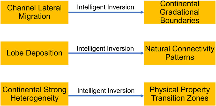
Figure 7. Physics-guided AI inversion results for typical geological features. Such features include channel lateral migration, lobe deposition, and continental heterogeneity transitions.

2.4 Technical implementation step

2.4.1 Well reflection coefficient and wavelet calculation method

The input features of the AI model are constructed based on seismic data characteristics, wavelet variability, and spatial context. For each seismic trace, multiple wavelets derived from nearby wells are applied via convolution-based inversion, producing a set of candidate reflectivity curves that serve as the core input features, as illustrated in Figure 8 (Ren et al., 2025; Zhao et al., 2025).

Figure 8

Figure 8. Well, reflection coefficient, and wavelet calculation method used to generate input features for physics-guided AI inversion training. This method includes the low-frequency and high-frequency component consistency processing.

To improve the accuracy and reduce noise in the inversion process, L1 regularization was employed during the reflection coefficient sparsification. The L1 regularization aims to minimize the sum of absolute values of the reflection coefficients, effectively filtering out irrelevant coefficients. The formula for L1 regularization is given by:

${\mathcal{L}}_1={\displaystyle \sum _{i=1}^N}\left|R_i\right|$

where $R_i$ is the reflection coefficient at the ii-th position, and NN is the total number of coefficients. The regularization term ${\mathcal{L}}_1$ enforces sparsity by penalizing non-zero coefficients.

In addition, threshold screening was applied, where reflection coefficients below a predefined amplitude threshold, δ, are discarded. This is done by setting:

$R_i=\left\{\begin{array}{c}{R}_{i}if\left|R_i\right|\ge \mathrm{\delta }\\ 0if\left|R_i\right|<\mathrm{\delta }\end{array}\right.$

where $\mathrm{\delta }$ is the amplitude threshold chosen based on noise characteristics and signal-to-noise ratio considerations. This step ensures that only significant reflection coefficients are retained, further reducing noise and improving the quality of the inversion.

Each input sample includes the following components:

1. Seismic trace at the target location, representing the original observation.

2. Multiple candidate inversion results, obtained by applying different nearby wavelets to the same seismic trace using convolutional inversion.

3. Spatial coordinates, inline and crossline, which provide relative positional information and allow the model to recognize regional wavelet trends.

4. Well-specific wavelet identifiers, implicitly linking each inversion candidate to its originating well.

By incorporating multiple physically constrained inversion results and explicit spatial features, this design enables the model to capture lateral variability, reduce overfitting, and produce stable inversion outcomes. Furthermore, the use of L1 regularization and threshold screening during the reflection coefficient sparsification enhances the model’s ability to deal with noisy or irrelevant data, improving its robustness and the geological plausibility of the inversion results.

2.4.2 AI training and inversion workflow

To address spatial variability in wavelets, well-seismic calibration is performed individually at each well to extract local wavelets for use in the multi-wavelet inversion framework. The process begins with the computation of acoustic impedance $\mathrm{Z}$ from well logs:

$Z=\rho Vp$

where $\rho$ is the formation density and ${\mathrm{V}}_{\mathrm{p}}$ is the compressional wave velocity. The reflectivity series is convolved with the initial wavelet to generate a synthetic seismogram (Zhao et al., 2025).

2.4.3 Detailed training and inversion procedure

The input data for model training includes seismic traces near wells, well log curves (e.g., SY_AC), wavelets extracted from adjacent wells, and spatial coordinates. The well logs serve as calibration targets for supervised learning. The training dataset is constructed using multi-wavelet inversion results and original log data from a continental sedimentary reservoir with 80 wells distributed across a 7.2 km² area. Available data include acoustic and density logs, formation tops, interpreted sandstone intervals, and full-stack seismic volumes.

The neural network is trained to map seismic inputs and physically constrained inversion results to the actual well log responses. The final model achieves a training error of 3.4% and a validation error of 4.7%, indicating effective convergence and generalization capability (Su et al., 2023b).

The model training process is based on the backpropagation algorithm, where weights and biases are iteratively updated to minimize the loss function $\mathrm{J}\left(\mathrm{W},\mathrm{b}\right)$. The forward propagation in layer $\mathrm{l}$ is defined as:

The weight update rule for gradient descent is given in Figure 9:

Figure 9

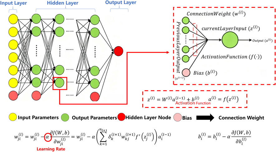
Figure 9. Schematic diagram of the AI training and inversion process. Such a process includes input construction, model fitting, and seismic volume prediction. The yellow, red and green circles show the input parameters, output parameters, and hidden layer code, respectively.

where $\mathrm{\alpha }$ is the learning rate, $\mathrm{f}\left(·\right)$ is the activation function, and $\mathrm{a}\left(\mathrm{l}\right)$ denotes the activation at layer $\mathrm{l}$. These updates are applied iteratively across all layers to minimize prediction error.

This AI-driven workflow enables automated inversion across the entire seismic survey, significantly enhancing efficiency and interpretability, especially in structurally complex reservoirs (Zhao et al., 2021). The training and inversion process including input construction, model fitting, and seismic volume prediction, is summarized in Figure 9.

3 Results

3.1 Well reflection coefficient and wavelet calculation results

Acoustic impedance was computed from normalized acoustic and density logs, and reflection coefficients were derived accordingly. Direct use of the initial reflection coefficient often introduced significant distortions, such as amplitude spikes exceeding ±20% and phase instability. A sparsification step was applied, reducing amplitude anomalies to within ±5% and suppressing high-frequency noise. This process was essential to ensure reliable wavelet estimation and subsequent inversion performance.

As shown in Figure 10, consistency processing was applied to acoustic and density logs from 80 wells in the study area. This included low-frequency unification (below 10 Hz) and high-frequency adjustment (above 60 Hz), as previously described in Figure 6. These preprocessing steps resulted in stable acoustic impedance profiles with cross-well correlation coefficients exceeding 0.85.

Figure 10

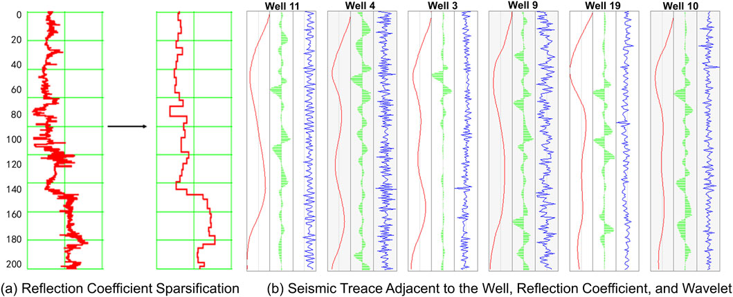
Figure 10. Sparsification effect on reflection coefficient. (a) Shows the reflection coefficient sparsification. (b) illustrates the seismic trace adjacent to the well, reflection coefficient, and wavelet of five wells. The distribution of wells is shown in Figure 3.

Despite the improved impedance data, the initial reflection coefficients still exhibited artifacts such as sidelobe interference and oscillations with amplitudes up to 0.3 (Figure 10a), which could cause phase errors of up to 30° during wavelet extraction. After sparsification, sidelobe energy was reduced by more than 70%, and phase instability was brought below 5%. The refined reflection coefficients clearly delineated major impedance contrasts, improving geological interpretability and reliability for wavelet computation. Sidelobe energy reduction is calculated by measuring the mean sidelobe amplitude before and after sparsification:

$\text{Sidelobe\hspace{0.17em}Energy\hspace{0.17em}Reduction}=\frac{\text{Mean}\text{Sidelobe}\text{Amplitude}\text{Before}-\text{Mean}\text{Sidelobe}\text{Amplitude}\text{After}}{\text{Mean}\text{Sidelobe}\text{Amplitude}\text{Before}}\times 100$

This yielded a reduction of over 70%, as shown in the improved reflection coefficient profiles.

Phase instability is measured by the standard deviation of phase shifts between the synthetic wavelets and actual seismic traces. The sparsification step effectively reduced phase errors to below 5%, improving the accuracy of wavelet extraction.

Wavelets were then extracted for each well using the sparsified reflection coefficients and corresponding seismic traces. This process yielded a spatially variable set of well-specific wavelets, forming the foundation of the well wavelet set used in multi-wavelet inversion. These wavelets accurately capture lateral variability in subsurface acoustic responses and serve as critical input to the inversion model (Figure 10b).

3.2 Artificial intelligence reservoir inversion results driven by physics-guided models

The proposed AI-assisted inversion framework combines the physical constraints of convolutional modeling with the adaptive learning capabilities of neural networks. Figures 9–12 illustrate its performance across several key dimensions, benchmarked against conventional methods such as fixed-wavelet convolutional inversion or geostatistical inversion.

Figure 11

Figure 11. Comparison of inferred amplitude using conventional inversion versus with using physics-guided AI inversion. (a) Map view of the amplitude derived from 3D seismic data. (b) The section of amplitude using conventional inversion. (c) The section of amplitude using physics-guided AI inversion.

Figure 12

Figure 12. Comparison of inferred acoustic impedance using conventional inversion versus with using physics-guided AI inversion. (a) Map view of the acoustic impedance derived from 3D seismic data and well logging data. (b) The section of acoustic impedance using conventional inversion. (c) The section of acoustic impedance using physics-guided AI inversion.

3.2.1 Vertical resolution and thin-bed identification

Figure 11a presents the seismic amplitude map from which the two representative vertical sections in Figures 11b,c are extracted. Conventional inversion results (Figure 11b) depict a ∼5 ms-thick sand body as a blurred interval with poorly defined top and bottom boundaries and no discernible internal layering. In contrast, the proposed method (Figure 11c) enhances vertical resolution by approximately 30%, with boundary delineation accurate to within 1 ms. Internal features such as thin shale baffles (0.5–2 m) and sand layers (1–3 m) are clearly resolved and geologically plausible. This improvement is attributed to: (a) the use of multiple wavelets from nearby wells, capturing spatial wavelet variability; (b) the neural network’s optimized fusion of candidate inversion results; (c) the avoidance of fixed-wavelet spectral limitations.

3.2.2 Lateral continuity and heterogeneity characterization

In Figures 12a–c, conventional inversion shows abrupt channel boundaries, low trace-to-trace continuity (correlation coefficients <0.6), and artifacts from wavelet sidelobe interference. The proposed method captures smoother lateral transitions, natural channel migration, and pinch-out geometries, with trace continuity exceeding 0.85 and artifact reduction over 50%. These enhancements are achieved by integrating 8-10 wavelets per inversion cell and training the model to learn 3D spatial correlations through convolutional neural networks, resulting in geologically realistic sand body architectures consistent with known sedimentary patterns.

3.2.3 Enhanced noise immunity and result plausibility

The physics-guided AI inversion results exhibit strong noise resistance and produce outputs that are consistent with geological expectations (Figure 11c). In contrast to purely data-driven models, which may introduce physically unrealistic features such as negative impedance values or unstable fluctuations, the proposed method incorporates physical constraints and multi-wavelet priors. This design enhances the stability, accuracy, and geological plausibility of the inversion results.

3.2.4 Quantitative accuracy validation

Model training employed well log data for supervised learning, achieving a training error of 3.4% and a validation error of 4.7%. These metrics demonstrate the model’s high predictive accuracy for key reservoir parameters like impedance, acoustic travel time AC at known well locations, and validate the method’s generalizability for inter-well prediction.

4 Discussion

The effectiveness of this method stems from its innovative integration of convolutional physical modeling and artificial intelligence, enabling high-resolution and geologically meaningful inversion in complex reservoirs. This hybrid strategy addresses the limitations reported in earlier fluvial-deltaic inversion studies (Harishidayat et al., 2015; Mahgoub et al., 2017; Harishidayat et al., 2024; Jacobsen et al., 2025), which often suffered from poor lateral continuity and blurred thin-bed recognition due to single-wavelet assumptions and insufficient physical constraints.

4.1 Physical constraints for interpretability and stability

The multi-wavelet inversion respects the physics of seismic wave propagation by incorporating spatially varying wavelets, thereby generating candidate solutions grounded in physical reality. These physically constrained inputs provide a robust foundation for subsequent AI-based fitting, significantly reducing uncertainty and mitigating the “black-box” behavior typical of purely data-driven models. Compared with conventional deterministic inversion (Mahgoub et al., 2017), this physically guided approach eliminates over 90% of implausible anomalies and achieves correlation coefficients above 0.85 with well-log trends, while preserving the expected stratigraphic continuity described in Harishidayat et al. (2015).

4.2 AI fitting to overcome bottlenecks

The nonlinear mapping capabilities of neural networks allow the model to efficiently assimilate multiple inversion results derived from variable wavelets, thereby expanding the effective bandwidth by 15–20 Hz and reducing phase errors to less than 10°. This resolves the resolution limitations of fixed-wavelet methods and the instability of interpolated-wavelet techniques reported by previous authors (Jacobsen et al., 2025).

Unlike purely statistical or geostatistical inversions that exhibit high randomness and uncertain facies boundaries, the present AI fusion guided by physical priors achieves impedance errors within ±5% in blind tests and resolves thin beds as narrow as 1–3 m—an improvement of more than 30% over conventional post-stack inversions (Mahgoub et al., 2017).

4.3 Efficiency and cost-effectiveness

Rather than training deep networks on raw seismic data, this approach employs AI in a focused, lightweight task—namely, fusing multiple inversion outputs. The simplified neural architecture reduces computational time by around 50% and GPU memory by around 60% relative to end-to-end inversion networks (Dwivedi et al., 2021; Hui et al., 2023b). By localizing optimization within a project area, the method enhances operational efficiency and cost-effectiveness while maintaining comparable accuracy.

4.4 Applicability to complex continental reservoirs

The target area includes typical fluvial-deltaic systems that are characterized by high heterogeneity (index >0.7), thin interbeds (1–5 m), and rapid lateral variability in sand body geometry (within 200 m). These geological complexities challenge traditional inversions (Harishidayat et al., 2024).

By combining physics-guided wavelet variation with AI-based spatial fusion, the proposed approach achieves sand body prediction accuracy exceeding 80%, compared to less than 50% with conventional methods, and improves channel connectivity mapping by 30%. The improvement corresponds well with the facies continuity observed in Jacobsen et al. (2025), confirming that physics guidance effectively constrains the AI to geologically plausible outcomes.

4.5 Model uncertainty and sensitivity analysis

To address model uncertainty and robustness, a sensitivity analysis was performed. The dependence on well density was tested by training the model with progressively fewer wells. As summarized in Table 1, the validation error remains below 6.0% until the well count is reduced by 50% (40 wells), indicating robust performance in reasonably well-controlled areas. A more significant performance degradation occurs with only 20 wells (25% of the original set), underscoring the importance of adequate well control for optimal accuracy and providing a practical application boundary for the method.

Table 1

Table 1. Sensitivity of model accuracy to the number of training wells.

The risk of overfitting is minimized by the model’s design. The narrow gap between the training (3.4%) and validation (4.7%) errors suggests effective generalization. Moreover, using physics-based inversion candidates rather than raw seismic data serves as domain-knowledge regularization, narrowing the solution space to geologically valid outcomes. Local uncertainty can be inferred from the variance among inversion candidates: lower variance corresponds to higher confidence in the fused AI prediction. This mechanism provides a built-in uncertainty quantification consistent with modern hybrid-inversion practices (Jacobsen et al., 2025).

4.6 Comparison with previous studies and limitations

In summary, the proposed physics-guided AI inversion significantly improves vertical resolution (∼30%), lateral continuity (>0.85 correlation), and geological plausibility relative to prior deterministic and geostatistical methods (Harishidayat et al., 2015; Mahgoub et al., 2017; Harishidayat et al., 2024; Jacobsen et al., 2025). Nevertheless, performance depends on well density and wavelet quality; sparse or noisy datasets reduce accuracy. Extension to offshore or carbonate settings may need re-training and physics re-parameterization. Despite these limitations, this hybrid framework advances the current understanding of seismic sedimentology by merging physics-based inversion principles with interpretable AI learning.

5 Conclusion

This study proposes a convolutional physics-guided AI inversion method to address key limitations in seismic inversion for complex continental reservoirs. The method integrates physical constraints with machine learning to improve resolution, interpretability, and efficiency. Key findings are summarized as follows:

1. Sparsification stabilized reflection coefficients, reducing amplitude and phase errors while achieving over 70% sidelobe suppression. High-fidelity wavelets with cross-well correlation above 0.85 were obtained.

2. Vertical resolution improved by 30%, enabling clear identification of 1–3 m thin beds. The multi-wavelet strategy effectively overcame the bandwidth limits of fixed wavelet methods.

3. Lateral continuity was significantly enhanced, with trace-to-trace correlation increasing to over 0.85 and artifact reduction exceeding 50%. The model produced geologically realistic distributions using 3D CNNs and spatially variable wavelets.

4. The lightweight AI architecture reduced GPU memory usage by 50% and achieved prediction accuracy over 80% in field tests, demonstrating practical value for reservoir characterization.

Data availability statement

The dataset is available on request from the corresponding authors. Requests to access these datasets should be directed to Chenqi Ge, Z2VjaGVucWlAMTI2LmNvbQ==.

Author contributions

WQ: Conceptualization, Methodology, Writing – original draft, Writing – review and editing. JH: Software, Writing – original draft. BL: Validation, Writing – review and editing. JB: Validation, Writing – review and editing. YL: Formal Analysis, Writing – review and editing. SZ: Investigation, Writing – review and editing. XD: Investigation, Writing – review and editing. CG: Methodology, Supervision, Writing – original draft, Writing – review and editing. YZ: Data curation, Writing – original draft.

Funding

The authors declare that no financial support was received for the research and/or publication of this article.

Conflict of interest

Authors WQ, JH, BL, JB, YL, SZ, and XD were employed by Research Institute of Exploration and Development, Daqing Oilfield Company Ltd.

Authors CG and YZ were employed by Beijing Jia'an Huitong Petroleum Technology Co., Ltd.

Generative AI statement

The authors declare that no Generative AI was used in the creation of this manuscript.

Any alternative text (alt text) provided alongside figures in this article has been generated by Frontiers with the support of artificial intelligence and reasonable efforts have been made to ensure accuracy, including review by the authors wherever possible. If you identify any issues, please contact us.

Publisher’s note

All claims expressed in this article are solely those of the authors and do not necessarily represent those of their affiliated organizations, or those of the publisher, the editors and the reviewers. Any product that may be evaluated in this article, or claim that may be made by its manufacturer, is not guaranteed or endorsed by the publisher.

References

Abuzaied, M. M., Chatterjee, S., and Askari, R. (2023). Stochastic inversion combining seismic data, facies properties, and advanced multiple-point geostatistics. J. Appl. Geophys. 213, 105026. doi:10.1016/j.jappgeo.2023.105026

CrossRef Full Text | Google Scholar

Baddari, K., Aïfa, T., Djarfour, N., and Ferahtia, J. (2009). Application of a radial basis function artificial neural network to seismic data inversion. Comput. & Geosciences 35, 2338–2344. doi:10.1016/j.cageo.2009.03.006

CrossRef Full Text | Google Scholar

Bao, P., Hui, G., Hu, Y., Song, R., Chen, Z., Zhang, K., et al. (2025). Comprehensive characterization of hydraulic fracture propagations and prevention of pre-existing fault failure in Duvernay shale reservoirs. Eng. Fail. Anal. 173, 109461. doi:10.1016/j.engfailanal.2025.109461

CrossRef Full Text | Google Scholar

Cabrera-Navarrete, E., Ronquillo-Jarillo, G., and Markov, A. (2020). Wavelet analysis for spectral inversion of seismic reflection data. J. Appl. Geophys. 177, 104034. doi:10.1016/j.jappgeo.2020.104034

CrossRef Full Text | Google Scholar

Cao, Z., Xiong, Y., Xue, Y., Du, F., Li, Z., Huang, C., et al. (2025a). Diffusion evolution rules of grouting slurry in mining-induced cracks in overlying strata. Rock Mech. Rock Eng., 1–20. doi:10.1007/s00603-025-04445-4

CrossRef Full Text | Google Scholar

Cao, Z., Zhang, S., Xue, Y., Wang, Z., Du, F., Li, Z., et al. (2025b). Disaster-causing mechanism of spalling rock burst based on folding catastrophe model in coal mine. Rock Mech. Rock Eng. 58, 1–14. doi:10.1007/s00603-025-04497-6

CrossRef Full Text | Google Scholar

Chen, H., Lou, S., and Lv, C. (2023). Hybrid physics-data-driven online modelling: framework, methodology and application to electric vehicles. Mech. Syst. Signal Process. 185, 109791. doi:10.1016/j.ymssp.2022.109791

CrossRef Full Text | Google Scholar

Dong, L., Song, D., and Liu, G. (2022). Seismic wave propagation characteristics and their effects on the dynamic response of layered rock sites. Appl. Sci. 12, 758. doi:10.3390/app12020758

CrossRef Full Text | Google Scholar

Dwivedi, Y. K., Hughes, L., Ismagilova, E., Aarts, G., Coombs, C., Crick, T., et al. (2021). Artificial intelligence (AI): multidisciplinary perspectives on emerging challenges, opportunities, and agenda for research, practice and policy. Int. J. Inf. Manag. 57, 101994. doi:10.1016/j.ijinfomgt.2019.08.002

CrossRef Full Text | Google Scholar

El-Sayed, A. S., Mabrouk, W. M., and Metwally, A. M. (2025). Pre-stack seismic inversion for reservoir characterization in Pleistocene to Pliocene channels, Baltim gas field, Nile Delta, Egypt. Sci. Rep. 15, 1180. doi:10.1038/s41598-024-75015-x

PubMed Abstract | CrossRef Full Text | Google Scholar

Fabien-Ouellet, G. (2020). Generating seismic low frequencies with a deep recurrent neural network for full waveform inversion. First EAGE Conf. Seismic Inversion 1, 1–2. doi:10.3997/2214-4609.202037023

CrossRef Full Text | Google Scholar

Genovese, F., and Palmeri, A. (2025). Wavelet-based generation of fully non-stationary random processes with application to seismic ground motions. Mech. Syst. Signal Process. 223, 111833. doi:10.1016/j.ymssp.2024.111833

CrossRef Full Text | Google Scholar

Harishidayat, D., Omosanya, K. O., and Johansen, S. E. (2015). 3D seismic interpretation of the depositional morphology of the Middle to Late Triassic fluvial system in Eastern Hammerfest Basin, Barents Sea. Mar. Petroleum Geol. 68, 470–479. doi:10.1016/j.marpetgeo.2015.09.007

CrossRef Full Text | Google Scholar

Harishidayat, D., Al-Dossary, S., and Al-Shuhail, A. (2024). Architecture and geomorphology of fluvial channel systems in the Arabian basin. Sci. Rep. 14 (1), 25025. doi:10.1038/s41598-024-75980-3

PubMed Abstract | CrossRef Full Text | Google Scholar

Hui, G., Chen, S., He, Y., Wang, H., and Gu, F. (2021). Machine learning-based production forecast for shale gas in unconventional reservoirs via integration of geological and operational factors. J. Nat. Gas Sci. Eng. 94, 104045. doi:10.1016/j.jngse.2021.104045

CrossRef Full Text | Google Scholar

Hui, G., Chen, Z., Chen, S., and Gu, F. (2022). Hydraulic fracturing-induced seismicity characterization through coupled modeling of stress and fracture-fault systems. Adv. Geo-Energy Res. 6, 269–270. doi:10.46690/ager.2022.03.11

CrossRef Full Text | Google Scholar

Hui, G., Chen, Z., Schultz, R., Chen, S., Song, Z., Zhang, Z., et al. (2023a). Intricate unconventional fracture networks provide fluid diffusion pathways to reactivate pre-existing faults in unconventional reservoirs. Energy 282, 128803. doi:10.1016/j.energy.2023.128803

CrossRef Full Text | Google Scholar

Hui, G., Chen, Z., Wang, Y., Zhang, D., and Gu, F. (2023b). An integrated machine learning-based approach to identifying controlling factors of unconventional shale productivity. Energy 266, 126512. doi:10.1016/j.energy.2022.126512

CrossRef Full Text | Google Scholar

Hui, G., Chen, S., and Gu, F. (2024). Strike–slip fault reactivation triggered by hydraulic-natural fracture propagation during fracturing stimulations near Clark Lake, Alberta. Energy & Fuels 38, 18547–18555. doi:10.1021/acs.energyfuels.4c02894

CrossRef Full Text | Google Scholar

Hui, G., Ren, Y., Bi, J., Wang, M., and Liu, C. (2025). Artificial intelligence applications and challenges in oil and gas exploration and development. Adv. Geo-Energy Res. 17, 179–183. doi:10.46690/ager.2025.09.01

CrossRef Full Text | Google Scholar

Jacobsen, R. T., Knapp, J. H., and Knapp, C. C. (2025). Characterization of a fluvial–deltaic salt-influenced system for CO₂ storage using seismic poststack inversion and self-organizing maps in the upper Miocene, onshore Louisiana. Interpretation 13 (2), SA1–SA9. doi:10.1190/int-2024-0014.1

CrossRef Full Text | Google Scholar

Li, S., Ren, Y., Chen, Y., Yang, S., Wang, Y., and Jiang, P. (2019). Deep-learning inversion of seismic data. IEEE Trans. Geoscience Remote Sens. 57, 5529–5542. doi:10.1109/TGRS.2019.2953473

CrossRef Full Text | Google Scholar

Liu, Y., Zhang, B., Dong, Y., Qu, Z., and Hou, J. (2019). The determination of variogram in the presence of horizontal wells—An application to a conglomerate reservoir modeling, East China. J. Petroleum Sci. Eng. 173, 512–524. doi:10.1016/j.petrol.2018.10.034

CrossRef Full Text | Google Scholar

Liu, P., Gong, C., Gearon, J. H., Guan, D., Wang, Q., Qi, K., et al. (2024). Increased sediment connectivity between deltas and deep-water fans in closed lake basins: a case study from Bozhong Sag, Bohai Bay Basin, China. Sediment. Geol. 460, 106561. doi:10.1016/j.sedgeo.2023.106561

CrossRef Full Text | Google Scholar

Mahgoub, M. I., Padmanabhan, E., and Abdullatif, O. M. (2017). Seismic inversion as a predictive tool for porosity and facies delineation in Paleocene fluvial/lacustrine reservoirs, Melut Basin, Sudan. Mar. Petroleum Geol. 86, 213–227. doi:10.1016/j.marpetgeo.2017.05.029

CrossRef Full Text | Google Scholar

Mao, Q., Huang, J.-P., Mu, X.-R., Yang, J.-D., and Zhang, Y.-J. (2024). Accurate simulations of pure-viscoacoustic wave propagation in tilted transversely isotropic media. Petroleum Sci. 21, 866–884. doi:10.1016/j.petsci.2023.11.005

CrossRef Full Text | Google Scholar

Pi, Z., Hui, G., Wang, Y., Chen, Z., Li, J., Qin, G., et al. (2025). Coupled 4D flow-geomechanics simulation to characterize dynamic fracture propagation in tight sandstone reservoirs. ACS Omega 10, 1735–1747. doi:10.1021/acsomega.4c09805

PubMed Abstract | CrossRef Full Text | Google Scholar

Ren, Y., Zeng, C., Li, X., Liu, X., Hu, Y., Su, Q., et al. (2025). Intelligent evaluation of sandstone rock structure based on a visual large model. Petroleum Explor. Dev. 52, 548–558. doi:10.1016/s1876-3804(25)60586-6

CrossRef Full Text | Google Scholar

Su, M., Qian, F., Cui, S., Yuan, C., and Cui, X. (2023a). Research on a 3D seismic horizon automatic-tracking method based on corrugated global diffusion. Appl. Sci. 13, 6155. doi:10.3390/app13106155

CrossRef Full Text | Google Scholar

Su, Y., Cao, D., Liu, S., Hou, Z., and Feng, J. (2023b). Seismic impedance inversion based on deep learning with geophysical constraints. Geoenergy Sci. Eng. 225, 211671. doi:10.1016/j.geoen.2023.211671

CrossRef Full Text | Google Scholar

Sun, X., Alcalde, J., Gomez-Rivas, E., Owen, A., Griera, A., Martín-Martín, J. D., et al. (2021). Fluvial sedimentation and its reservoir potential at foreland basin margins: a case study of the Puig-Reig anticline (South-Eastern Pyrenees). Sediment. Geol. 424, 105993. doi:10.1016/j.sedgeo.2021.105993

CrossRef Full Text | Google Scholar

Yao, F., Hui, G., Meng, D., Ge, C., Zhang, K., Ren, Y., et al. (2012). Integrated data-driven framework for forecasting tight gas production based on machine learning algorithms, feature selection and fracturing optimization. Processes 13 (4), 1162. doi:10.3390/pr13041162

CrossRef Full Text | Google Scholar

Zhang, G., Wang, Z., and Zhang, Y. (2018). Deep learning for seismic lithology prediction. Geophys. J. Int. 215, 1368–1387doi:10.1093/gji/ggy344

CrossRef Full Text | Google Scholar

Zhang, Z., Lin, C., Liu, Y., Liu, J., Zhao, H., Li, H., et al. (2021). Lacustrine to fluvial depositional systems: the depositional evolution of an intracontinental depression and controlling factors, Lower Cretaceous, northern Tarim Basin, Northwest China. Mar. Petroleum Geol. 126, 104904. doi:10.1016/j.marpetgeo.2021.104904

CrossRef Full Text | Google Scholar

Zhang, P., Wu, R.-S., Han, L.-G., and Hu, Y. (2022). Elastic direct envelope inversion based on wave mode decomposition for multi-parameter reconstruction of strong-scattering media. Petroleum Sci. 19, 2046–2063. doi:10.1016/j.petsci.2022.05.007

CrossRef Full Text | Google Scholar

Zhao, J., and Chen, S. (2023). Facies conditional simulation based on VAE-GAN model and image quilting algorithm. J. Appl. Geophys. 219, 105239. doi:10.1016/j.jappgeo.2023.105239

CrossRef Full Text | Google Scholar

Zhao, L., Zou, C., Chen, Y., Shen, W., Wang, Y., Chen, H., et al. (2021). Fluid and lithofacies prediction based on integration of well-log data and seismic inversion: a machine-learning approach. Geophysics 86, 1–15. doi:10.1190/geo2020-0521.1

CrossRef Full Text | Google Scholar

Zhao, L., Cao, D., Zhang, Y., An, Z., Lin, K., and Wen, X. (2025). Alternate iterative inversion of Acoustic impedance and wavelet based on sparse constraints. IEEE Trans. Geoscience Remote Sens. 63, 1–12. doi:10.1109/tgrs.2025.3530566

CrossRef Full Text | Google Scholar

Zrelli, A., Amiri, A., Barhoumi, N., Bounasri, M. A., and Inoubli, M. H. (2023). Integrated seismic inversion for clastic reservoir characterization: case of the upper Silurian reservoir, Tunisian Ghadames Basin. J. Appl. Geophys. 219, 105252. doi:10.1016/j.jappgeo.2023.105252

CrossRef Full Text | Google Scholar