 Margaret F. J. Dolan
 Lilja R. Bjarnadóttir
- Earth Surface and Seabed Department, Geological Survey of Norway (NGU), Trondheim, Norway
Seamounts are a prime example of an ecologically relevant marine landform. They are internationally recognized by the OSPAR commission as a threatened and/or declining habitat yet estimates of their distribution in Norwegian waters are not adequately reported in databases used for ocean management. Here we describe mapping of the distribution of seamounts and related topographic highs, conducted for Norway’s offshore seabed mapping program MAREANO. We employ a combination of automated methods to detect, delineate and characterize peaks and associated areas of elevated terrain from the GEBCO global bathymetry data compilation. The resulting broad-scale (1:2,000 000) map includes seamounts (over 1,000 m high), lower knolls and mounds as well as many ridges, several of which are of comparable height to seamounts. Our results include hundreds of topographic highs not reported by previous studies as well as confirming and further characterizing many known features through geomorphometric analysis. This new information contributes to documentation of seabed geodiversity and provides timely data for international reporting and knowledge-based ocean management supporting sustainable development of offshore resources, following SDG14 (Life Below Water). The maps serve as baseline information for further scientific studies, including characterization of the associated benthic habitats which will ultimately help define appropriate management measures.
1 Introduction
Seamounts are commonly defined as subcircular topographic highs more than 1,000 m above the surrounding seabed (Dove et al., 2020; Stagpoole and Mackay, 2022) but sometimes include lower features and a variety of forms (Staudigel et al., 2010). They have been mapped by several global (Gevorgian et al., 2023; Harris et al., 2014; Kitchingman and Lai, 2004; Yesson et al., 2011; Yesson et al., 2021) and regional (Morato et al., 2013) studies which report occurrences in Norwegian waters. These estimates vary, and may over- or under-estimate the prevalence of seamounts in this area depending on the data, methods and definitions used.
From an ecological perspective, topographic features which extend higher into the water column are typically subject to different biophysical regimes than the surrounding seabed. Benthic habitats on these elevated features tend to reflect these variations (e.g., Hanz et al., 2021; Meyer et al., 2023; Roberts et al., 2018). The OSPAR1 commission is the intergovernmental organization coordinating efforts to protect the marine environment of the North-East Atlantic. OSPAR defines seamounts as undersea mountains with crests rising more than 1,000 m above the surrounding seabed (OSPAR, 2008), and recognizes them as a threatened and/or declining habitat. Currently less than ten seamounts are included in the OSPAR’s collated records of threatened and/or declining habitats in Norwegian waters (OSPAR, 2024a; OSPAR, 2024b). OSPAR-related reports (Kutti et al., 2019; OSPAR, 2010; 2022) nevertheless mention additional features over 1,000 m high in this area. Shaded relief images further indicate the presence of numerous topographic highs, particularly in the deep Norwegian Sea near the Arctic Mid-Ocean Ridge (AMOR). Some of these features are over the height threshold for OSPAR seamounts, while smaller features are important in a wider ecosystem and habitat context (Rogers, 2018) and fall within some seamount definitions (Staudigel et al., 2010).
Here we present the results of broad-scale (1:2,000 000) mapping of seamounts and related topographic highs from bathymetry data within all areas included in recent management plans for Norwegian sea areas (Ministry of Climate and Environment, 2020). These results are produced for Norway’s national offshore seabed mapping program–MAREANO (Bøe et al., 2020) which provides ecosystem relevant maps and data across the Norwegian shelf, slope and deep sea to support knowledge-based management. Interest in sustainable development of ocean resources (Ministry of Trade Industry and Fisheries, 2024) is especially high in large parts of our study area, particularly where designated vulnerable and valuable areas (Eriksen et al., 2021) overlap areas of fisheries interest (Ministry of Trade Industry and Fisheries, 2024) or those opened for seabed mineral related activities (Ministry of Energy, 2024). Our results provide timely information for national management, international reporting (e.g., OSPAR) and scientific study.
We employ a combination of automated methods for detection and delineation of seamounts and related topographic highs from compiled bathymetry data. Our analysis further discriminates between these elevated features based on depth attributes, morphology and the underlying data quality. Here we outline the workflows used and present selected results from the study to support online maps published by the Geological Survey of Norway for MAREANO.
2 Methods
2.1 Study area
The study area covers all areas included in recent management plans for Norwegian sea areas (Ministry of Climate and Environment, 2020), Figure 1. This includes areas claimed by Denmark and the newly ratified Faroese areas. The area includes several physiographic regions shaped by various geological processes through millions of years (Gaina et al., 2025), including multiple glaciations through the Quaternary ice ages (Ramberg et al., 2008). The deep parts of the Norwegian Sea, which extend to depths of nearly 6,000 m, consist of oceanic crust and are a result of the opening of the North Atlantic Ocean. Slow rifting, with accompanying volcanic and hydrothermal activity, is still occurring along the AMOR (Stubseid et al., 2023) which runs from Jan Mayen north and into the Arctic Ocean, while the Aegir Ridge to the southeast of Jan Mayen is inactive. The rugged AMOR is hundreds to thousands of meters high, with a rift valley at the center and sparsening topographic highs to either side. By comparison the Lofoten, Greenland, Nansen and Norwegian basins are relatively flat-bottomed. Meanwhile, the formerly glaciated continental shelves of the North Sea, Norwegian Sea and Barents Sea exhibit a dominance of glacial influence which is evident in the seabed stratigraphy and morphology. Banks, valleys, moraines and other glacial features are commonplace (Ottesen et al., 2005).
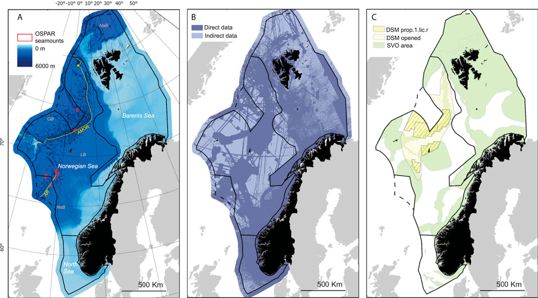
Figure 1. Overview maps of the study area showing (A) Color shaded relief GEBCO_2024 bathymetry and registered OSPAR seamounts (OSPAR, 2024b). (B) Reclassified GEBCO_2024 TID grid showing direct and indirect data. (C) Area designations for deep sea mineral activities (Ministry of Energy, 2024): DSM opened–the areas open for deep sea mineral activities; DSM prop.1.lic.r.: Proposed areas for the 1. licensing round for deep sea mineral exploration. SVO area–particularly vulnerable and valuable areas (Eriksen et al., 2021). Management areas (Ministry of Climate and Environment, 2020; Ministry of Climate and Environment, 2024) are outlined in black with the earlier boundary shown as a dashed line which includes areas no longer under Norway’s jurisdiction. The location of major sea areas is shown in (A) NaB, Nansen Basin; LB, Lofoten Basin; GB, Greenland Basin; NoB, Norwegian Basin. Spreading ridges including the Arctic Mid Ocean Ridge–AMOR and Aegir ridge AR are shown in yellow, source (Gevorgian et al., 2023 accompanying data). The yellow star indicates the position of Norway’s deepest point Molloy Deep (5,569 m). The 1,000 m depth contour is shown in blue for reference. Map projection: north pole stereographic.
2.2 Bathymetry data
Multibeam bathymetry data, facilitating the production of digital terrain models (≤50 m resolution) are available for large parts of Norway’s seabed, but do not cover all areas of interest for this study. We have therefore used the global bathymetry data compilation GEBCO (Mayer et al., 2018) as a basis for this broad-scale analysis. Specifically, we use the GEBCO_2024 15-arc second grid (GEBCO Compilation Group, 2024) which incorporates all MAREANO’s 2019 multibeam bathymetry in the deep Norwegian Sea as well as earlier data managed by the Norwegian Mapping Authority and other contributors. GEBCO_2024’s accompanying type identifier (TID) grid (Figure 1B) indicates the type of source data at each location, primarily separating between direct and indirect measurements or other unknown sources. To facilitate our analysis GEBCO_2024 data for the study area were projected to north pole stereographic projection and resampled to 500 m resolution. Although this resampling generalizes the topographic information from multibeam data, where available, the 500 m raster remains suitable for detection of features measuring at least 1 km (Tobler, 1987), which is smaller than the minimum feature size we aim to detect (Section 2.3.2).
2.3 Feature detection and delineation
We employ a combination of analysis tools to identify relevant topographic features and classify them by morphology and other attributes relevant to MAREANO’s end users. The complementary approaches used include raster analyses, feature delineation and filtering routines, each of which are outlined below and summarized in Figure 2 (see also Supplementary Material).
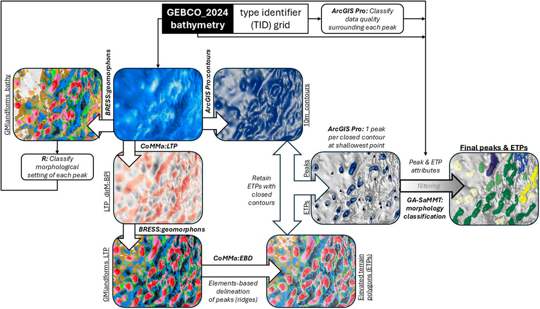
Figure 2. Overview of the detection and delineation workflow. Tools for the main workflows are shown in bold italics, other operations described in italics, intermediate and final datasets are underlined. In the geomorphons figures peaks (CoMMa:EBD core geomorphons) are shown in red and ridges (CoMMa:EBD subordinate geomorphons) are shown in pink, for colors of the remaining landforms see Supplementary Figure S3. See Figures 2, 3 for colors of final peaks and ETPs.
2.3.1 Preparatory raster analyses
2.3.1.1 Local topographic position
Using the CoMMa toolbox for ArcGIS Pro (Arosio et al., 2024; Gafeira et al., 2024) we generate a local topographic position (LTP) derivative from the bathymetry data which reports the height relative to a mean or median value within a local analysis neighborhood. When dealing with sloping terrain and complex length scales a directional median approach can offer a better estimate of relative position than standard median- or mean-based indices (Gafeira et al., 2024; Kim and Wessel, 2008). Here we create a Directional Median Bathymetry Position Index (dirM-BPI) LTP (Arosio et al., 2024; Gafeira et al., 2024), hereinafter referred to as LTP_dirM-BPI, which reports the height relative to the lowest (least biased) median value occurring in N “bow-tie” sectors within a circular analysis neighborhood (Kim and Wessel, 2008). Following Kim and Wessel’s (2008) recommendations we set the analysis neighborhood to have a diameter roughly twice the size of the expected size of most features of interest. Although our data indicates undersea mountains spanning a range of sizes within the study area, through visual assessment we confirmed that the 20 km radius analysis neighborhood used by Morato et al.’s (2013) study of seamounts in the NE Atlantic is a good general estimate. Consequently LTP_dirM-BPI was calculated using a 20 km radius and, as per the CoMMa v.1.2 implementation, with N = 8 sectors.
2.3.1.2 Geomorphons
As with previous seamount mapping studies, the first step is detection of peaks. Several approaches can be adopted, typically harnessing hydrological and/or neighborhood/focal statistics (e.g., Harris et al., 2014; Kitchingman and Lai, 2004; Morato et al., 2013; Yesson et al., 2011; Yesson et al., 2021). Geomorphons (Jasiewicz and Stepinski, 2013) is a machine vision approach to distinguishing morphometric features from elevation data based on principles of openness and pattern recognition. It is well suited to the current study and is computationally more efficient than neighborhood/focal approaches. Using geomorphons ten common landform elements (flat, peak, ridge, shoulder, slope, convex slope [spur], concave slope [hollow], footslope, valley and pit) are typically recognized. This classified output can be used to delineate areas of elevated terrain associated with the peaks, and to characterize their morphological setting.
Here we use the BRESS toolbox (Masetti et al., 2018; Masetti, 2024) implementation of the geomorphon algorithm. This incorporates Jasiewicz and Stepinski’s (2013) original method and includes some spatial generalization of the output landforms based on texton theory. Geomorphon outputs are dependent on several user-defined settings as well as the input data. Here we employ settings and data that facilitate emphasis of ridges and peaks since these are the landform elements most relevant for onward delineation of seamounts and related topographic highs.
To highlight these peaks and ridges we apply geomorphon analysis not to the bathymetry but to the LTP_dirM-BPI surface (Section 2.3.1.1), to produce the GMlandforms_LTP raster (Supplementary Table S1). This is an effective approach for delineating certain morphological features (Arosio et al., 2024) and can help overcome data artefacts (Gafeira et al., 2024). We use an analysis neighborhood with the same outer radius as for the LTP_dirM-BPI calculation. An inner radius of 5 km helps minimize (local-scale) artefacts while preserving relevant (broad-scale) features, and the flatness threshold is set at one. A second geomorphon analysis was applied to the bathymetry data directly (Supplementary Table S1), this time with a flatness threshold of two to strike a good balance between detection of real features and artefacts. This GMlandforms_bathy output indicates natural landform elements and is used to classify the mapped features in terms of their neighboring terrain, separating those occurring in otherwise flat areas from those in rugged areas. The onward use of each of these two geomorphons outputs is summarized in Figure 2.
2.3.2 Delineation of elevated terrain
The landform output (GMlandforms_LTP) from the BRESS analysis of the LTP_dirM-BPI derivative is used to delineate polygons, hereinafter referred to as Elevated Terrain Polygons (ETPs), encompassing connected areas of elevated terrain associated with each detected peak. We apply Elements-Based Delineation in CoMMa v.1.2 (CoMMa:EBD) to create polygons capturing this elevated terrain (see Supplementary Table S2 for settings applied). Selecting peaks as the core geomorphons and ridges as subordinate geomorphons we restrict the delineation to elevated areas directly associated with peaks. Including additional subordinate geomorphons (e.g., slopes) is counterproductive, resulting in large areas of connected elevated terrain being delineated rather than individual areas of elevated terrain directly associated with each peak. Additional settings restrict the dimensions and degree of polygon generalization applied such that we produce an output suitable for a 1:2,000 000 map product. Since our primary goal is to detect prominent topographic highs, while avoiding limitations associated with the compiled bathymetry data the minimum detectable height is set at 200 m, and the minimum width set at 2 km. This width setting is more conservative than the theoretically attainable (Tobler, 1987) minimum detectable feature size of 1 km (1:1,000 000) from 500 m raster data. This is because we add the condition that ETPs are at least 4 cells wide to ensure reliable detection and generalization, especially given the variation in the quality of the underlying bathymetry data.
2.3.3 Refining mapped features
2.3.3.1 Filtering ETPs
The output ETPs fulfill CoMMa:EBD settings and are linked to the flatness threshold and radii used in the geomorphon analysis. However, many ETPs are indistinct features and/or are not pertinent due to their location, form or dimensions. We first remove internal holes in the ETPs using a fixed area threshold suited to the 1:2,000 000 mapping scale. A series of filtering operations is then applied so that only relevant ETPs remain (Supplementary Material Section S1; Supplementary Table S3). To facilitate this filtering process, we use 10 m contours generated from the GEBCO_2024 bathymetry. Using spatial joins, we retain only ETPs containing closed contours. Dissolved versions of these closed contour polygons are then used for further filtering and creation of peak points.
2.3.3.2 Peak points
Rather than estimating peak locations using polygon centroids (e.g., Morato et al., 2013) we create points at the minimum depth for each dissolved contour polygon within the ETPs (Section 1). These peak points are used to summarize attributes of interest. Due to large variations in data quality within the study region, which affect both delineation and contouring, our peak positions are indicative only. They serve as a companion to the ETPs but may differ from the registered position of named features (IHO-IOC, 2025) or peaks reported by other studies.
2.4 Feature attributes
Characterization of the peaks and polygons provide information which helps to highlight similarities and differences between them. Here we describe some key attributes; see also Supplementary Material for more information on specific attributes and the summary information in Supplementary Tables S4, S5.
2.4.1 Height above the surrounding seabed
For each peak point and ETP we assign a measure of its height relative to the surrounding seabed. This relative height is later classified to separate mountains and ridges over 1,000 m high from lower features. Since the LTP_dirM-BPI inherently compares height relative to a base height represented by the lowest value of the directional median within the analysis neighborhood (Section 2.3.1.1) this gives a suitable indicator of height for the present study. By extracting the maximum value of LTP_dirM-BPI for each closed contour polygon (each of which contains a single peak point) we obtain an estimate of the height of each peak relative to the surrounding seabed. This approximation produces a reasonable height estimate for features occurring on sloping terrain, due to the directional approach (Kim and Wessel, 2008), without compromising estimates for flat terrain. It also minimizes issues with single spurious values which are often linked to artefacts in compiled datasets like GEBCO_2024. For polygons the relative height is taken as the maximum value of LTP_dirM-BPI within the entire ETP. See Supplementary Section S3, Figure S1 for further information and a discussion of alternative height metrics considered.
2.4.2 Peaks - source data quality
The quality of the underlying bathymetry is an important indicator of confidence in the mapped features. We use a reclassified version of the GEBCO_2024 TID grid (Section 2.1) with sub-codes for different measurement types merged to a 3-category raster–direct, indirect and unknown. This is analyzed using zonal statistics within a 20 km buffer around each peak point to summarize the majority, count and percentage of cells in each category. The unknown category is virtually absent within our study area and hence does not feature in our categorization. Each peak is then classified based on the majority value within the 20 km buffer and its percentage within the analysis neighborhood (Direct: >90% majority direct; Partial: 50%–90% majority direct; Indirect: majority (>50%) indirect). See Supplementary Material Section S4; Supplementary Figures S2 for further information on this topic.
2.4.3 Peaks - neighboring terrain classification
In geological and ecological contexts, it is useful to know if a seamount candidate is a distinct feature on an otherwise flat seabed, or if it occurs in rugged terrain. To produce a classification of the morphological setting of a peak in relation to its neighboring terrain we use the geomorphon landforms generated directly from the bathymetry (GMlandforms_bathy) (Section 2.3.1.1; Supplementary Table S2). We compute a composition signature of the percentage cover of each of the ten landform classes occurring in this raster within a 20 km buffer around each peak using the “motif” package (Nowosad, 2021) in R. This signature is then converted to a distance object using the Jensen-Shannon distance method and hierarchical clustering applied.
2.4.4 Polygons - morphology classification
The delineated ETPs comprise a variety of shapes and sizes. Basic attributes summarizing properties such as their width to length ratio is incorporated in the output from CoMMa:EBD. The toolbox also offers the possibility to generate further attributes which may be useful in characterizing features for onward interpretation (e.g., Arosio et al., 2023) but it currently stops short of performing a morphology classification per se. By contrast, the GA-SaMMT toolbox (Huang et al., 2023) includes routines specifically directed to characterizing and classifying morphology. It generates multiple attributes towards this end based on input polygons, bathymetry data and derivatives. Classification in GA-SaMMT v.1.2 is possible for a selection of morphological features from the two-part morphology/geomorphology classification system developed by the International Seabed Geomorphology Mapping working group (ISGM - formerly MIM-GA) (Dove et al., 2016; Dove et al., 2020; Nanson et al., 2023). We applied the various steps in GA-SaMMT for characterizing topographic highs and classifying their morphology, which takes a hierarchal rule-based approach (Huang et al., 2023). Slight modifications were made to the default settings and workflows (see Supplementary Material Section S2). Most importantly we use the relative heights from LTP_dirM-BPI at the morphology classification stage rather than simple depth ranges. This ensures that the morphological classifications are consistent with our other attributes for height above the surrounding seabed.
3 Results
Our analysis produces two datasets.
• Points representing the main peaks of topographic highs including seamounts, knolls, mounds and ridges.
• Polygons (ETPs) delineating the elevated terrain associated with each peak. Note that an ETP may contain several peaks representing the main topographic highs within the structure.
Here we present example maps and summary statistics to give an overview of the results and some key attributes (see also Data Availability Statement and Supplementary Material).
3.1 Peaks
3.1.1 Peak height
Our analysis identified 974 peaks occurring in 754 ETPs within the study area (Figure 3). They are distributed throughout the deep Norwegian Sea with the greatest densities close to the AMOR and several occurrences in the Barents Sea. All these features could be considered seamounts depending on the definition used (Staudigel et al., 2010). In this study features which exceed 1,000 m in height are of particular interest (OSPAR candidates), but lower features are also relevant. We therefore preserve and categorize lower peaks into those with relative heights of 500–1,000 m, and 200–500 m. Figure 3C illustrates how the peak points are distributed within the delineated polygons and closed contours. More than one peak may occur within a polygon, but only a single peak may occur for each closed contour group. From Figure 3B we see that over half the peaks are less than 500 m high, while few are over the 1000 m threshold. Further details per height class are shown in Figure 3D.
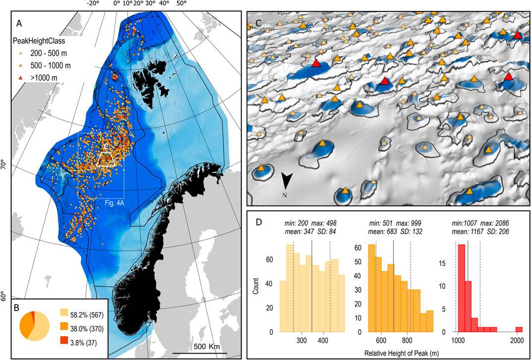
Figure 3. (A) Overview map showing peaks symbolized by height class with GEBCO_2024 color shaded bathymetry (depth range 0–5,931 m), Norway and management plan areas in black. Map projection: north pole stereographic. (B) Pie chart showing peak counts and percentages by height class. (C) Example 3D map extract (see A for location) showing closed contours (blue) and polygon outlines (black) with peaks superimposed–note varied detail of topography due to data quality (D) Histogram for relative heights of peaks per height class. Mean (solid line) and standard deviation (SD) (dotted line) values for each class are indicated and maximum and minimum values listed for each height class. The extent of Figure 4A is indicated for reference. Symbolization by other peak attributes is available in the online maps (see Data Availability Statement) with examples in Supplementary Material.
3.1.2 Neighboring terrain
Through hierarchical classification of geomorphon landform composition signatures we find that the first two clusters effectively separate distinct features from those occurring on rugged terrain (Supplementary Figure S3). The former may be more likely to differ in terms of environmental conditions from their surrounding seabed and includes a far greater proportion of flat seabed within the surrounding 20 km buffer.
3.1.3 Source data quality
At a regional level the quality issues related to the compiled GEBCO_2024 data have a relatively minor impact on our overall results but can lead to some features being missed, their shape being misclassified or their height estimate misleading. Due to the importance of this uncertainty for onward use of the output maps we summarize these uncertainties for end-users by attributing the peaks with the quality of the source data surrounding them (see Supplementary Material Section S4; Supplementary Figures S2 for further information) including visualization of mosaic plots (Meyer et al., 2006; Meyer et al., 2024) comparing data quality with peak height and neighboring terrain. Comparison with shaded relief images further highlights differences in data quality in terms of degree to which topographic features are resolved, as well as the potential influence of data artefacts. It is important to note that this uncertainty is also linked to the quality of the containing ETP.
3.2 Elevated Terrain Polygons (ETPs)
Figure 4A shows the ETPs for a portion of the study area, illustrating how the peak points complement the polygons, showing the location of the main summits within each ETP (Figure 4C). Across the entire study area, the proportions of ETPs in each height class are similar to those for the peaks, differing in numbers because some ETPs contain multiple peaks. Although GA-SaMMT’s morphology classification can currently discriminate between ten types of topographic highs, just four categories (mounds, knolls, seamounts and ridges) are recognized within our study area, based on our ETPs and the settings applied. The proportions of different morphological feature classifications within each height category (Figure 4B) confirm that over half of the highest features (>1,000 m relative height) are morphometrically classified not as seamounts, but as ridges due to their high length/width ratios.
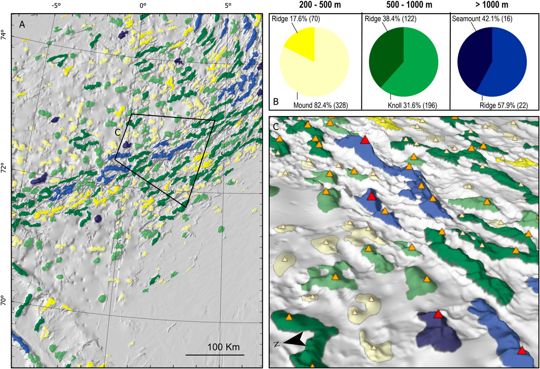
Figure 4. (A) Map extract (see Figure 3 for location) showing ETPs symbolized by their morphological classification (colors as per (B)). Map projection: north pole stereographic. (B) Pie charts showing relative proportions of each morphological feature per height class. (C) 3D map extract showing how peaks are located in relation to ETPs symbolized by morphology (see A for location).
4 Discussion
Our combined method effectively identifies, classifies and delineates the elevated terrain associated with the peaks of relevant undersea mountains where a single approach would have been less successful. Geomorphons offers a convenient and effective method for initial identification of candidate peaks and for characterizing the morphological setting of the mapped features. We adapted settings and applied preprocessing to avoid data-related issues as far as possible but cannot overcome the fact that the true topographic complexity of features is undetected in indirect data, and hence by geomorphons analysis. At locations where direct and indirect data meet, particularly where the direct data are single multibeam lines, challenging alignment of the depth values in the GEBCO_2024 grid leads to artefacts or unnaturally resolved features. These are detected as spurious landforms by geomorphons and related analyses. Our filtering routines helped to minimize the impact of such data on the final map.
Delineation of features was important here with a view to potential OSPAR reporting. Multiple approaches were tested for delineation of the ETPs with the aim of finding a method that does more than approximate the base area of each feature (e.g., Yesson et al., 2021), but which stops short of detailed delineation of individual geomorphological landforms (sensu Nanson et al., 2023). Combining geomorphons analysis and delineation routines, the CoMMa toolbox offers a convenient workflow. As with any automated approach, there is scope for improving the delineated features by manual editing, but this is beyond the scope of the present broad-scale study. The resulting 1:2,000 000 scale ETPs are well matched to the areal extent, underlying data and user needs. They effectively indicate the main areas of elevated terrain associated with peaks of seamounts and related topographic highs visible in the GEBCO_2024 data. These ETPs will appear generalized if viewed at finer map scales and/or together with higher resolution bathymetry data. Detailed delineation and geological interpretation are done separately as part of the Geological Survey of Norway’s regional scale (1:100,000–1:250,000) landform mapping for MAREANO within prioritized areas where multibeam data and supporting geological information are available. Additional in-situ information allows MAREANO to further characterize the associated benthic habitats.
Besides topographic complexity the true dimensions of topographic highs are often underestimated where they are detected within indirect or partial bathymetry data. Differences in data quality affect the reliability of LTPs and associated height estimates. Nevertheless, our selected metric of height above the seabed (LTP_dirM-BPI) works well for varying quality data across different types of terrain and where the data resolution is coarse with respect to the delineated polygons, (cf. Smith et al., 2009) see also Supplementary Section S3, Supplementary Figure S1. It is also in good general agreement with the IHO-IOC feature categorization for most existing named features. Our maps employ strict height categories relevant to widely used classifications, but the value of relative height as estimated by LTP_dirM-BPI is retained in the attribute table for flexibility. This is important since there is uncertainty associated with the height values, particularly in areas with indirect data. Furthermore, there is a lack of consensus on how ecologically relevant the somewhat arbitrary, yet practical, height thresholds for seamounts are. Additional depth attributes allow the peaks and polygons also to be assessed in relation to other data and ecological influences such as their relation to water masses (Jeansson et al., 2017) and other oceanographic processes (Hanz et al., 2021; Roberts et al., 2018) which may influence benthic habitats (Meyer et al., 2023).
4.1 Seamount candidates
It is important to strike a good balance between over- and under-estimating the prevalence of seamounts and related features, especially where the results will be used for conservation planning and sustainable management. Due consideration of the underlying data and methods employed is also important, e.g., now superseded data (Harris et al., 2014; Morato et al., 2013; Yesson et al., 2011); number of peaks reported per topographic high (Yesson et al., 2021). The recent global study by Gevorgian et al. (2023) based on the vertical gravity gradient (VGG) (Sandwell et al., 2021) has helped highlight seamount peaks as far north as 80° and is in good general agreement with our results. We nevertheless detect several hundred ETPs and associated peaks which are not documented in previous studies. Most of these newly mapped features have a relative height of under 500 m (none are over 1,000 m). We report 38 ETPs with a relative height of over 1,000 m which may be considered for inclusion in the OSPAR database. For all but one of these features (where the highest peak within the closed contour polygon was 996 m rather than 1,000 m within the entire ETP) the height classification matches that of the highest peak contained in the ETP. Nine of these 38 are currently registered in OSPAR including seven within the present Norwegian management area (Ministry of Climate and Environment, 2024), which is reduced in area from the earlier boundary delimiting our study area (see section 2.1). Eight additional ETPs are within 20 m of this height limit and could be considered if there is some flexibility in the threshold.
Several previously reported seamounts noted in OSPAR, (2022) coincide with our ridges over 1,000 m. ISGM morphology definitions (Dove et al., 2020) do not discriminate between ridges of different heights hence there is no separation of ridges by height in GA-SaMMT-based classification, nor can a feature be both a ridge and a seamount due to the hierarchical approach (Huang et al., 2023). Ridge-like seamounts are to be expected in a setting such as the AMOR where they are formed by geological processes in the rift zone (Stubseid et al., 2023). We therefore consider our ridge-ETPs over 1,000 m to be of interest, alongside the seamount-ETPs as OSPAR seamount candidates. Indeed, several already-registered OSPAR seamounts are represented by ridge-ETPs in our results. We see a similar proportion of ridge-shaped features of moderate (500–1,000 m) height but fewer lower features take this form. We expect ridges to be less prominent on older, more sedimented structures away from the rift zone, but indirect data are also more widespread in these areas with features poorly resolved.
Vector maps of the distribution of seamounts and related topographic highs provide important baseline information and help highlight and quantify these ecologically relevant landforms visible in shaded relief images. Since our analysis is based on automated methods the results may be readily updated to take advantage of new data incorporated in future revisions of GEBCO. This may include, but is not limited to, extensive multibeam data being acquired in the deep Norwegian Sea by The Norwegian Offshore Directorate 2024–2025. Our maps can inform follow-up scientific studies, ecodiversity estimates, conservation planning (e.g., Eriksen et al., 2021; Legrand et al., 2024), regional habitat (Ramirez-Llodra et al., 2024) and status assessments (OSPAR, 2022) as well as national red-listing of landforms and nature types (Artsdatabanken, 2018). More generally such landform maps contribute essential geodiversity information (Schrodt et al., 2019; Dolan et al., 2022). This is particularly important to support sustainable development in line with SDG 14, especially in regions where it is challenging to align the needs of industry and conservation against a background of incomplete knowledge.
Data availability statement
Publicly available (GEBCO_2024) bathymetry data were analyzed in this study: https://www.gebco.net/data-products-gridded-bathymetry-data/gebco2024-grid. The results from this study are available from Geonorge, Norway’s national repository for geospatial data: https://www.geonorge.no/en/. Please enter the search term "Undersea mountains" to access the data.
Author contributions
MD: Writing – review and editing, Formal Analysis, Writing – original draft, Methodology, Visualization, Conceptualization. LB: Project administration, Writing – review and editing, Methodology, Conceptualization.
Funding
The authors declare that financial support was received for the research and/or publication of this article. This work was supported by the MAREANO program and the Geological Survey of Norway.
Acknowledgements
We thank Aave Lepland for invaluable assistance with symbology and online publication of the results of this study. We also wish to thank the reviewers for constructive comments which helped improve this manuscript.
Conflict of interest
The authors declare that the research was conducted in the absence of any commercial or financial relationships that could be construed as a potential conflict of interest.
Generative AI statement
The author(s) declare that no Generative AI was used in the creation of this manuscript.
Any alternative text (alt text) provided alongside figures in this article has been generated by Frontiers with the support of artificial intelligence and reasonable efforts have been made to ensure accuracy, including review by the authors wherever possible. If you identify any issues, please contact us.
Publisher’s note
All claims expressed in this article are solely those of the authors and do not necessarily represent those of their affiliated organizations, or those of the publisher, the editors and the reviewers. Any product that may be evaluated in this article, or claim that may be made by its manufacturer, is not guaranteed or endorsed by the publisher.
Supplementary material
The Supplementary Material for this article can be found online at: https://www.frontiersin.org/articles/10.3389/feart.2025.1690996/full#supplementary-material
Footnotes
1OSPAR is named after the OSlo and PARis conventions of 1972 and 1974 respectively, now superseded by the 1992 OSPAR convention.
References
Arosio, R., Wheeler, A., Sacchetti, F., Guinan, J., Benetti, S., O'Keeffe, E., et al. (2023). The geomorphology of Ireland's Continental shelf. J. Maps 19 (1), 2283192. doi:10.1080/17445647.2023.2283192
Arosio, R., Gafeira, J., De Clippele, L., Wheeler, A., Huvenne, V., Sacchetti, F., et al. (2024). CoMMa: a GIS geomorphometry toolbox to map and measure confined landforms. Geomorphology 458, Article 109227. doi:10.1016/j.geomorph.2024.109227
Artsdatabanken (2018). Norsk rødliste for naturtyper 2018. Available online at: https://www.artsdatabanken.no/rodlistefornaturtyper (Accessed June 27, 2025).
Bøe, R., Bjarnadóttir, L. R., Elvenes, S., Dolan, M., Bellec, V., Thorsnes, T., et al. (2020). Revealing the secrets of Norway's seafloor–geological mapping within the MAREANO programme and in coastal areas, 505. London: Geological Society. doi:10.1144/SP505-2019-82
Dolan, M., Bøe, R., and Bjarnadóttir, L. R. (2022). Delivering seabed geodiversity information through multidisciplinary mapping initiatives: experiences from Norway. GEUS Bull. 52. doi:10.34194/geusb.v52.8325
Dove, D., Bradwell, T., Carter, G., Cotterill, C., Gafeira Goncalves, J., Green, S., et al. (2016). Seabed geomorphology: a two-part classification system. Br. Geol. SurvAvailable online at: https://nora.nerc.ac.uk/id/eprint/514946/1/Seabed_Geomorpholgy_classification_BGS_Open_Report.pdf
Dove, D., Nanson, R., Bjarnadóttir, L., Guinan, J., Gafeira, J., Post, A., et al. (2020). A two-part seabed geomorphology classification scheme:(v. 2). Part 1: morphology features glossary. doi:10.5281/zenodo.4071939
Eriksen, E., van der Meeren, G. I., Nilsen, B. M., von Quillfedt, C., and Johnsen, H. (2021). Særlig verdifulle og sårbare områder (SVO) i norske havområder - miljøverdi. En gjennomgang av miljøverdier og grenser i eksisterende SVO og forslag til nye områder. IMR Rep. 2021-26. Available online at: https://www.hi.no/hi/nettrapporter/rapport-fra-havforskningen-2021-26.
Gafeira, J., Arosio, R., and Laurence, D. C. (2024). ricarosio/CoMMa: Comma toolbox v1.2 (CoMMa1_2). doi:10.5281/zenodo.11109024
Gaina, C., Jakobsson, M., Straume, E. O., Timmermans, M. L., Boggild, K., Bünz, S., et al. (2025). Arctic Ocean bathymetry and its connections to tectonics, oceanography and climate. Nat. Rev. Earth and Environ. 6, 211–227. doi:10.1038/s43017-025-00647-0
Gevorgian, J., Sandwell, D. T., Yu, Y., Kim, S. S., and Wessel, P. (2023). Global distribution and morphology of small seamounts. Earth Space Sci. 10 (4), Article e2022EA002331. doi:10.1029/2022ea002331
Hanz, U., Roberts, E., Duineveld, G., Davies, A., van Haren, H., Rapp, H., et al. (2021). Long-term observations reveal environmental conditions and food supply mechanisms at an arctic deep-sea sponge ground. J. Geophys. Res. - Oceans 126 (3), e2020JC016776. doi:10.1029/2020JC016776
Harris, P. T., Macmillan-Lawler, M., Rupp, J., and Baker, E. K. (2014). Geomorphology of the oceans. Mar. Geol. 352, 4–24. doi:10.1016/j.margeo.2014.01.011
Huang, Z., Nanson, R., Mcneil, M., Wenderlich, M., Gafeira, J., Post, A., et al. (2023). Rule-based semi-automated tools for mapping seabed morphology from bathymetry data. Front. Mar. Sci. 10, Article 1236788. doi:10.3389/fmars.2023.1236788
IHO-IOC (2025). IHO-IOC GEBCO gazetteer of undersea feature names. Available online at: www.gebco.net.
Jasiewicz, J., and Stepinski, T. F. (2013). Geomorphons - a pattern recognition approach to classification and mapping of landforms. Geomorphology 182, 147–156. doi:10.1016/j.geomorph.2012.11.005
Jeansson, E., Olsen, A., and Jutterström, S. (2017). Arctic intermediate water in the nordic seas, 1991–2009. Deep Sea Res. Part I Oceanogr. Res. Pap. 128, 82–97. doi:10.1016/j.dsr.2017.08.013
Kim, S., and Wessel, P. (2008). Directional median filtering for regional-residual separation of bathymetry. Geochem. Geophys. Geosystems 9. doi:10.1029/2007GC001850
Kitchingman, A., and Lai, S. (2004). Inferences on potential seamount locations from mid-resolution bathymetric data. Editors T. Morato, and D. Pauly Seamounts: Biodiversity and Fisheries. Fisheries Centre Research Reports 12(5).(Vancouver: University of British Columbia), 7–12.
Kutti, T., Windsland, K., Broms, C., Falkenhaug, T., Biuw, M., Thangstad, T. H., et al. (2019). Seamounts in the OSPAR maritime area-from species to ecosystems. IMR Rep. 2019 – 42. Available online at: https://www.hi.no/hi/nettrapporter/rapport-fra-havforskningen-en-2019-42
Legrand, E., Boulard, M., O'Connor, J., and Kutti, T. (2024). Identifying priorities for the protection of deep-sea species and habitats in the nordic seas.
Masetti, G. (2024). BRESS v.2.5.2. Available online at: https://www.hydroffice.org/bress/main.
Masetti, G., Mayer, L. A., and Ward, L. G. (2018). A Bathymetry- and reflectivity-based approach for seafloor segmentation. Geosciences 8 (1), 14. doi:10.3390/geosciences8010014
Mayer, L., Jakobsson, M., Allen, G., Dorschel, B., Falconer, R., Ferrini, V., et al. (2018). The nippon Foundation-GEBCO seabed 2030 project: the quest to see the World's oceans completely mapped by 2030. Geosciences 8 (2), 63. doi:10.3390/geosciences8020063
Meyer, D., Zeileis, A., and Hornik, K. (2006). The strucplot framework: visualizing multi-way contingency tables with VCD. J. Stat. Softw. 17 (3). doi:10.18637/jss.v017.i03
Meyer, H. K., Davies, A. J., Roberts, E. M., Xavier, J. R., Ribeiro, P. A., Glenner, H., et al. (2023). Beyond the tip of the seamount: distinct megabenthic communities found beyond the charismatic summit sponge ground on an arctic seamount (schulz bank, arctic mid-ocean ridge). Deep Sea Res. Part I Oceanogr. Res. Pap. 191, 103920. doi:10.1016/j.dsr.2022.103920
Meyer, D., Zeileis, A., Hornik, K., and Friendly, M. (2024). Vcd: visualizing categorical data_. R package version 1.4-13. Available online at: https://CRAN.R-project.org/package=vcd.
Ministry of Climate and Environment. (2020). Meld. St. 20 (2019–2020). Norway’s integrated ocean management plans — barents sea–lofoten area; the Norwegian Sea; and the north sea and Skagerrak.
Ministry of Climate and Environment (2024). “Meld. St. 21 (2023–2024). Norway’s integrated ocean management plans,” in Barents sea–lofoten area; the Norwegian Sea; and the north sea and Skagerrak.
Ministry of Energy (2024). Opening of areas for mineral activities on parts of the Norwegian Continental shelf. Available online at: https://www.regjeringen.no/en/topics/energy/oil-and-gas/kunnskapsinnhenting-og-konsekvensutredning/opening-of-areas-for-mineral-activities-on-parts-of-the-norwegian-continental-shelf/id2871504/(Accessed June 27, 2025).
Ministry of Trade Industry and Fisheries (2024). Næringsplan for norske havområder. Available online at: https://www.regjeringen.no/no/dokumenter/naringsplan-for-norske-havomrader/id3046882/(Accessed June 27, 2025).
Morato, T., Kvile, K. O., Taranto, G. H., Tempera, F., Narayanaswamy, B. E., Hebbeln, D., et al. (2013). Seamount physiography and biology in the north-east Atlantic and Mediterranean Sea. Biogeosciences 10 (5), 3039–3054. doi:10.5194/bg-10-3039-2013
Nanson, R., Arosio, R., Gafeira, J., McNeil, M., Dove, D., Bjarnadóttir, L., et al. (2023). A two-part seabed geomorphology classification scheme; part 2: geomorphology classification framework and glossary. doi:10.5281/zenodo.7804019
Nowosad, J. (2021). Motif: an open-source R tool for pattern-based spatial analysis. Landsc. Ecol. 36 (1), 29–43. doi:10.1007/s10980-020-01135-0
OSPAR (2008). Case reports for the OSPAR list of threatened And/Or declining species and habitats Available online at: https://www.ospar.org/site/assets/files/44271/seamounts.pdf.
OSPAR (2010). Background document for seamounts. Available online at: https://www.ospar.org/work-areas/bdc/species-habitats/list-of-threatened-declining-species-habitats/habitats/seamounts.
OSPAR (2022). Status assessment 2022 - seamounts. BDC2022/seamounts. Available online at: https://oap.ospar.org/en/ospar-assessments/committee-assessments/biodiversity-committee/status-assesments/seamounts/.
OSPAR (2024a). OSPAR habitats in the north-east Atlantic Ocean - 2022 point records v2022. Dataset 1. Available online at: https://emodnet.ec.europa.eu/geonetwork/srv/eng/catalog.search#/metadata/2f1d91d7-4d81-448b-8df8-8080dbde372eJNCC (Accessed June 27, 2025).
OSPAR (2024b). OSPAR habitats in the north-east Atlantic Ocean - 2022 polygon records v2022. Available online at: https://emodnet.ec.europa.eu/geonetwork/srv/eng/catalog.search#/metadata/53704f1d-5efd-45e0-bae3-9ec611baea40JNCC (Accessed June 27, 2025).1
Ottesen, D., Dowdeswell, J. A., and Rise, L. (2005). Submarine landforms and the reconstruction of fast-flowing ice streams within a large Quaternary ice sheet: the 2500-km-long Norwegian-Svalbard margin (57–80 N). Geol. Soc. Am. Bull. 117 (7-8), 1033–1050. doi:10.1130/b25577.1
Ramberg, I. B., Bryhni, I., Nøttvedt, A., and Rangnes, K. (2008). “The making of a land,” in Geology of Norway. Geological society of Norway.
Ramirez-Llodra, E., Meyer, H., Bluhm, B., Brix, S., Brandt, A., Dannheim, J., et al. (2024). The emerging picture of a diverse deep Arctic Ocean seafloor: from habitats to ecosystems. Elementia-science Anthropocene 12 (1), 00140. doi:10.1525/elementa.2023.00140
Roberts, E., Mienis, F., Rapp, H., Hanz, U., Meyer, H., and Davies, A. (2018). Oceanographic setting and short-timescale environmental variability at an arctic seamount sponge ground. Deep-Sea Res. Part I – Oceanogr. Res. Pap. 138, 98–113. doi:10.1016/j.dsr.2018.06.007
Rogers, A. (2018). The biology of seamounts: 25 years on. Adv. Mar. Biol. 79, 137–224. doi:10.1016/bs.amb.2018.06.001
Sandwell, D., Harper, H., Tozer, B., and Smith, W. (2021). Gravity field recovery from geodetic altimeter missions. Adv. Space Res. 68, 1059–1072. doi:10.1016/j.asr.2019.09.011
Schrodt, F., Bailey, J. J., Kissling, W. D., Rijsdijk, K. F., Seijmonsbergen, A. C., Van Ree, D., et al. (2019). To advance sustainable stewardship, we must document not only biodiversity but geodiversity. Proc. Natl. Acad. Sci. 116 (33), 16155–16158. doi:10.1073/pnas.1911799116
Smith, M., Rose, J., and Gousie, M. (2009). The cookie cutter: a method for obtaining a quantitative 3D description of glacial bedforms. Geomorphology 108 (3-4), 209–218. doi:10.1016/j.geomorph.2009.01.006
Stagpoole, V., and Mackay, K. (2022). Cookbook for generic terms of undersea feature names. Available online at: https://iho.int/uploads/user/Inter-Regional%20Coordination/GEBCO/SCUFN/MISC/Cookbook_for_Generic_Feature_terms_v1.1_May%202021.pdf.
Staudigel, H., Koppers, A., Lavelle, J., Pitcher, T., and Shank, T. (2010). Defining the word seamount. Oceanography 23 (1), 20–21. doi:10.5670/oceanog.2010.85
Stubseid, H., Bjerga, A., Haflidason, H., Pedersen, L., and Pedersen, R. (2023). Volcanic evolution of an ultraslow-spreading ridge. Nat. Commun. 14 (1). doi:10.1038/s41467-023-39925-0
Tobler, W. (1987). “Measuring spatial resolution,” in Proceedings, land resources information systems conference. Beijing, 12–16.
Yesson, C., Clark, M. R., Taylor, M. L., and Rogers, A. D. (2011). The global distribution of seamounts based on 30 arc seconds bathymetry data. Deep-Sea Res. Part Oceanogr. Res. Pap. 58 (4), 442–453. doi:10.1016/j.dsr.2011.02.004
Keywords: seamounts, landforms, marine geology, geomorphology, geomorphometry, GIS, GEBCO bathymetry, SDG #14
Citation: Dolan MFJ and Bjarnadóttir LR (2025) Seamounts and related topographic highs – automated mapping in support of sustainable ocean management, Norway. Front. Earth Sci. 13:1690996. doi: 10.3389/feart.2025.1690996
Received: 22 August 2025; Accepted: 13 October 2025;
Published: 18 November 2025.
Edited by:
Sheng Nie, Chinese Academy of Sciences (CAS), ChinaReviewed by:
Zhi Huang, Geoscience Australia, AustraliaShenghao Shi, Fisheries and Oceans Canada (DFO), Canada
Copyright © 2025 Dolan and Bjarnadóttir. This is an open-access article distributed under the terms of the Creative Commons Attribution License (CC BY). The use, distribution or reproduction in other forums is permitted, provided the original author(s) and the copyright owner(s) are credited and that the original publication in this journal is cited, in accordance with accepted academic practice. No use, distribution or reproduction is permitted which does not comply with these terms.
*Correspondence: Margaret F. J. Dolan, bWFyZ2FyZXQuZG9sYW5Abmd1Lm5v