Feasibility study of logging-while-drilling boundary detection using electric dipole antenna

The critical need for deep boundary detection in complex hydrocarbon reservoirs drives the advancement of Logging-while-drilling (LWD) azimuthal electromagnetic measurement (AEM). New deep detection tools employ open-loop half-circle electric dipole (ED) antennas that enable longer-distance detection compared to traditional closed-loop magnetic dipole (MD) antennas, owing to the unique advantages of electric field signals in azimuthal resolution and amplitude attenuation. However, a significant research gap remains as the reception efficiency of ED antennas is largely unaccounted for. Existing theoretical analyses simplistically assume 100% efficiency, identical to closed-loop MD antennas. In reality, the actual reception efficiency of ED antennas may cause signal attenuation in new deep detection tools, which could compromise boundary identification accuracy and pose a risk to real-time geosteering. To address this issue, this paper investigates the feasibility of boundary detection using ED antennas in LWD by developing a comprehensive framework that integrates antenna characterization, reception efficiency simulation, and depth of detection (DOD) evaluation. The research first compares the attenuation characteristics and resistivity response of ED and MD antennas in homogeneous media. It then reveals the influence mechanisms governing ED antenna reception efficiency, identifying formation resistivity as the dominant factor while demonstrating the negligible effects of operating frequency and relative permittivity in typical low-frequency applications. Furthermore, comparative analysis in single-boundary formations confirms that the new deep detection tool exhibits significantly superior azimuthal sensitivity and a DOD exceeding twice that of traditional tools, even when efficiency attenuation is accounted for. This work provides the theoretical and empirical evidence necessary to validate ED antennas for reliable deep boundary detection, enhancing the safety and accuracy of geosteering in complex environments.

1 Introduction

Azimuthal Logging-while-drilling (LWD) electromagnetic (EM) tools, characterized by inherent azimuthal sensitivity, enable the detection of formation boundaries within a radial range of several meters around the borehole (Bell et al., 2006; Bittar et al., 2009). These tools serve as critical instruments for offshore oilfields and unconventional complex reservoir exploration (Liu Y. et al., 2023; Wang et al., 2025b). For decades, LWD tools have exclusively utilized closed-loop antennas. These antennas excite EM fields within formations, with subsequent formation evaluation relying on the propagation and attenuation characteristics of these fields (Kang et al., 2022a; Wang L. et al., 2025; Wu et al., 2025). Given that antenna dimensions are typically negligible relative to operational wavelengths, they can be mathematically approximated as magnetic dipole (MD) antennas (Wu et al., 2022a; Kang et al., 2022b). Essentially, traditional EM logging tools acquire formation-boundary information through analysis of magnetic field components emitted from MD sources (Wu et al., 2022b; Qiao et al., 2024; Zhao et al., 2025). However, their depth of detection (DOD) is constrained by the transmitter-to-receiver (T–R) spacing and operating frequency (f). Consequently, DOD enhancement is typically achieved by extending T–R spacing while reducing operating frequency.

With continuous research advancement and rapid technological developments, hybrid dipole measurement methods integrating electric and magnetic field measurements have been progressively adopted in LWD applications. Li (2018) demonstrated that electric fields exhibit superior sensitivity to far-field formation anomalies, proposing novel deep-detection approaches through electric field data acquisition. Hagiwara (2018) established electric dipole (ED) measurements as an effective solution for look-around geosteering applications Wang et al. (2020) introduced an ultra-deep detection method based on hybrid dipoles, leveraging both the electric and magnetic fields excited by MD sources to achieve effective detection of formation features distant from the borehole under short-spacing configuration.

While these previous studies have successfully demonstrated the sensitivity advantage of electric field measurements for deep detection, they have not fully considered the practical reception efficiency of the open-loop antennas. This is a critical oversight, as theoretical analyses typically assume an ideal 100% reception efficiency for closed-loop antennas, an assumption that is extended to new tools without justification. Consequently, while traditional deep detection tools with MD antennas can disregard the impact of reception efficiency on signals, this is not the case for new tools which consist of closed-loop MD transmitting antennas and open-loop half-circle ED receiving antennas. The actual reception efficiency of ED antennas may cause signal attenuation in these tools, thereby affecting real-time boundary detection during logging operations. Therefore, to address this specific gap, accounting for antenna reception efficiency is of critical importance for the systematic investigation into the feasibility of ED antennas for LWD boundary detection applications.

This study investigates the feasibility of ED antenna-based boundary detection in LWD and presents a simulation method for ED antenna reception efficiency. The work aims to validate the boundary detection capability of ED antennas and to clarify the actual DOD of new deep detection tools. The rest of this paper is organized as follows. Firstly, the basic structure and measurement principles of deep detection tools are introduced, with comparison of ED and MD antenna attenuation characteristics in homogeneous media and their resistivity characterization capabilities. Then, key factors affecting ED antenna reception efficiency are examined based on attenuation characteristics differences. Secondly, azimuthal sensitivity of ED and MD antennas in single-boundary formations is compared to verify ED antenna-based boundary detection feasibility. Finally, simulation cases demonstrate the actual boundary detection capability of new deep detection tools when accounting for antenna reception efficiency, with direct comparison to traditional deep detection tools.

2 Methodology and simulation analysis

2.1 Tool configuration and measurement principles

Traditional LWD EM tools employ a single-transmitter-dual-receiver coaxial antenna configuration. During LWD operations, the axial transmitting antenna excites EM fields in formations, with formation resistivity measurement achieved through amplitude attenuation (Att) and phase shift (PS) of propagating EM waves (Wang et al., 2025a). Since traditional LWD EM tools adopt a coaxial antenna design that utilizes only the coaxial magnetic field component, they lack azimuthal information for geosteering applications. To address this limitation, traditional deep detection tools incorporate tilted antennas as receivers (see Figure 1a), which enhance azimuthal sensitivity by adding cross-component magnetic field signals. Meanwhile, new deep detection tools employ open-loop half-circle ED antennas as receivers (see Figure 1b), further improving azimuthal sensitivity through cross-component electric field signals (Wang et al., 2024). Specifically, by measuring induced electromotive force (EMF) at receivers under different tool rotation angles, the acquired signals can be converted into Att geosignal (G_Att) and PS geosignal (G_PS), enabling effective detection of formation boundaries:

${\mathit{G}}_{\mathit{A}\mathit{t}\mathit{t}}=20{\lg }_{10}\frac{\text{sqrt}\left({\left[\text{Re}\left({\mathit{V}}_{\mathit{\beta }}\right)\right]}^2+{\left[\text{Im}\left({\mathit{V}}_{\mathit{\beta }}\right)\right]}^2\right)}{\text{sqrt}\left({\left[\text{Re}\left({\mathit{V}}_{\mathit{\beta }+\mathit{\pi }}\right)\right]}^2+{\left[\text{Im}\left({\mathit{V}}_{\mathit{\beta }+\mathit{\pi }}\right)\right]}^2\right)}(1)$

${\mathit{G}}_{\mathit{P}\mathit{S}}={\tan }^{-1}\frac{\text{Im}\left({\mathit{V}}_{\mathit{\beta }}\right)}{\text{Re}\left({\mathit{V}}_{\mathit{\beta }}\right)}-{\tan }^{-1}\frac{\text{Im}\left({\mathit{V}}_{\mathit{\beta }+\mathit{\pi }}\right)}{\text{Re}\left({\mathit{V}}_{\mathit{\beta }+\mathit{\pi }}\right)}(2)$

In Equation 1 and Equation 2, Re[⋅] and Im[⋅] denote the real part and imaginary part functions, respectively; V denotes the induced EMF at the receiving antenna, and β is the tool rotation angle.

Figure 1

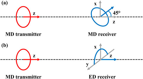
Figure 1. Antenna configuration of deep detection tools. (a) Traditional tool (b) New tool.

In new deep detection tools, the total induced EMF measured by the open-loop half-circle ED antenna represents the integral of the electric field along the semicircular path. To reduce computational costs and simplify modeling, inversion, and data processing, existing studies equate the total induced EMF of the open-loop half-circle ED antenna to the superposition of EMFs measured separately by a half closed-loop MD antenna and an ED antenna (Wang et al., 2022). Although this equivalence holds in terms of induced EMF, it does not imply physical equivalence between the open-loop half-circle ED antenna and the superposition model. Consequently, the feasibility of open-loop half-circle ED antennas for boundary detection requires further investigation.

2.2 Attenuation characteristics of ED and MD antennas in homogeneous media

The primary objectives during LWD operations are accurate measurement of formation boundaries and resistivity to enable real-time geosteering and well trajectory control (Zhao et al., 2018; Zhang et al., 2025). Accomplishing these objectives increasingly involves not only improved tool design but also advanced computational interpretation, where accurate forward models serve as the foundation for sophisticated inversion schemes using, for example, efficient inversion framework (Zhan et al., 2024; Luo et al., 2025) or advanced wave-equation solvers (Zhan et al., 2021; Liu Q. Q. et al., 2023). In homogeneous media, the azimuthal signal of tools is zero. However, formation resistivity can be determined by measuring the induced EMF at receivers, leveraging the sensitivity of the coaxial magnetic field component (Hzz) to resistivity. To investigate the attenuation characteristics of open-loop half-circle ED antennas in homogeneous media and their resistivity characterization capability, this section establishes an infinitely thick homogeneous formation model with resistivity Rt ranging from 1 to 100 Ω·m. Transmitters employ closed-loop MD antennas, while receivers use either tilted closed-loop MD antennas or open-loop half-circle ED antennas, all with a radius of 0.05 m. Given that deep detection tools typically utilize longer T–R spacing and lower operating frequencies to enhance DOD, with reference to the Schlumberger Geosphere, this study sets the T–R spacing to 10 m and the operating frequencies from 6 to 48 kHz. By comparing EMF responses of tilted closed-loop MD antennas and open-loop half-circle ED antennas under varying resistivities across frequencies, the applicability of ED antennas for resistivity measurement is validated.

Figure 2 illustrates the EMF responses of tilted closed-loop MD antennas and open-loop half-circle ED antennas versus formation resistivity in a homogeneous formation model with 10 m T–R spacing at frequencies of 6, 12, 24, and 48 kHz. As resistivity increases, the induced EMF of both antennas enhances, with higher frequencies generating larger EMF magnitudes. Although the MD antenna exhibits stronger signal intensity, both antennas demonstrate consistent variation patterns. This indicates that ED antennas share similar attenuation characteristics to closed-loop MD antennas in homogeneous media, confirming their robust applicability for formation resistivity measurement through EM wave amplitude and phase analysis. Given the lower signal strength of ED antennas compared to MD antennas, and considering that the actual reception efficiency of ED antennas may cause tool signal attenuation, we will further investigate key factors affecting ED antenna reception efficiency.

Figure 2

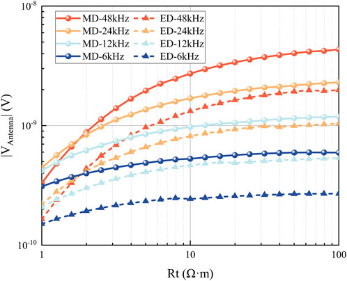
Figure 2. EMF responses in relation to formation resistivity for MD and ED antennas in homogeneous media.

2.3 Concept of antenna reception efficiency

The new deep detection tool employs a closed-loop MD antenna as the transmitter and an open-loop half-circle ED antenna as the receiver. Since the reception/transmission efficiency of closed-loop antennas is typically assumed to be 100%, further analysis of their efficiency is unnecessary. According to the reciprocity theorem, antenna efficiency exhibits symmetry whether the antenna operates as a transmitter or receiver (Štumpf, 2016). Therefore, this section simulates the reception efficiency of the open-loop half-circle ED antenna based on the reciprocity theorem. By simulating its transmission efficiency (i.e., antenna efficiency η), we equivalently evaluate its reception efficiency, thereby accurately assessing the actual received signal of the new deep detection tool.

Antenna efficiency (η) is a fundamental metric for evaluating antenna performance. It is defined as the ratio of the power radiated into external space (i.e., the power effectively transformed into EM waves) to the active power delivered to the antenna at the feed port of the radio-frequency circuit. Mathematically, it is expressed as the ratio of the radiated power to the input power, formally expressed as:

$\mathit{\eta }=\frac{\mathit{P}}{{\mathit{P}}_{\mathit{max}}}(3)$

In Equation 3, P denotes the actual power radiated externally by the antenna, and P_max represents the theoretical maximum power achievable when the antenna impedance Z matches the characteristic impedance Z_ref of the coaxial cable.

The terms P and P_max are defined in Equations 4, 5, respectively:

$\mathit{P}=\frac{1}{2}\text{Re}\left(\mathit{V}·{\mathit{I}}^{*}\right)(4)$

${\mathit{P}}_{\mathit{max}}=\frac{{\mathit{V}}_0^2}{2·{\mathit{Z}}_{\mathit{r}\mathit{e}\mathit{f}}}(5)$

Where V₀ denotes the excitation voltage, set to 1 V in this study.

The antenna impedance Z and the characteristic impedance Z_ref of the coaxial cable are defined in Equations 6, 7, respectively:

$\mathit{Z}=\frac{\mathit{V}}{\mathit{I}}(6)$

${\mathit{Z}}_{\mathit{r}\mathit{e}\mathit{f}}=\frac{\sqrt{{\mathit{\mu }}_0}}{2\mathit{\pi }}·\frac{1}{\sqrt{{\mathit{\epsilon }}_{\mathit{r}}{\mathit{\epsilon }}_0}}\log \left(\frac{{\mathit{b}}_{\mathit{c}\mathit{o}\mathit{a}\mathit{x}}}{{\mathit{a}}_{\mathit{c}\mathit{o}\mathit{a}\mathit{x}}}\right)(7)$

where μ₀ is the magnetic permeability of vacuum, ε₀ is the electric permittivity of vacuum, ε_r is the relative permittivity of the coaxial cable dielectric, which was set to 2.07 in this study. b_coax is the inner radius of the coaxial cable’s outer conductor, and a_coax is the radius of the coaxial cable’s inner conductor. The characteristic impedance Z_ref was set to the standard value of 50 Ω. It is important to note that the explicit geometry of the coaxial cable structure was not modeled. Instead, a simplified excitation was applied by imposing a uniform voltage difference across the antenna feed faces, which induces the requisite electromagnetic fields and surface currents.

The calculation of antenna efficiency using Equation 3 through Equation 7 relies on two key assumptions: a lossless transmission line feed and perfect electric conductor (PEC) antenna materials. These assumptions ensure that the characteristic impedance is real and that all power loss is attributed to impedance mismatch radiation, rather than feed or conductor losses.

The key to antenna efficiency lies in the impedance matching between Z and Z_ref. When these impedances are matched, maximum power transfer is theoretically achieved, leading to ideal antenna efficiency. However, the antenna impedance is influenced by factors such as antenna structure, dimensions, shape, and the surrounding medium, and varies with operating frequency. Consequently, these factors directly impact the antenna efficiency. Therefore, this study establishes a detailed 3D model of the open-loop half-circle ED antenna to investigate the influence mechanisms of operating frequency, formation resistivity, relative permittivity, and antenna arm length on the antenna’s reception efficiency.

3 Simulation of ED antenna reception efficiency

3.1 Antenna model

The arm length of a dipole antenna is typically designed to be a quarter-wavelength (λ/4), as antenna efficiency is closely related to wavelength in air. Ideally, at a quarter-wavelength, the current distribution along a dipole antenna approximates a sinusoidal waveform (see Figure 3a), with minimum current at the ends and maximum current at the center. This distribution favors the formation of an ideal radiation pattern, thereby maximizing radiation efficiency. Accordingly, a detailed 3D model of the open-loop half-circle ED antenna was constructed (see Figure 3b). This antenna consists of two dipole arms, each being a quarter-toroid of radius R (i.e., antenna arm length L = πR/2), with a cross-sectional radius of R/20. A small cylindrical gap of size R/100 between the arms represents the voltage source. The surrounding medium domain is modeled as a free-space sphere of radius 2.4R, truncated by a perfectly matched layer (PML) with a thickness of 0.48R (one-tenth of the sphere’s diameter) to absorb outgoing radiation and minimize spurious reflections from the domain boundaries.

Figure 3

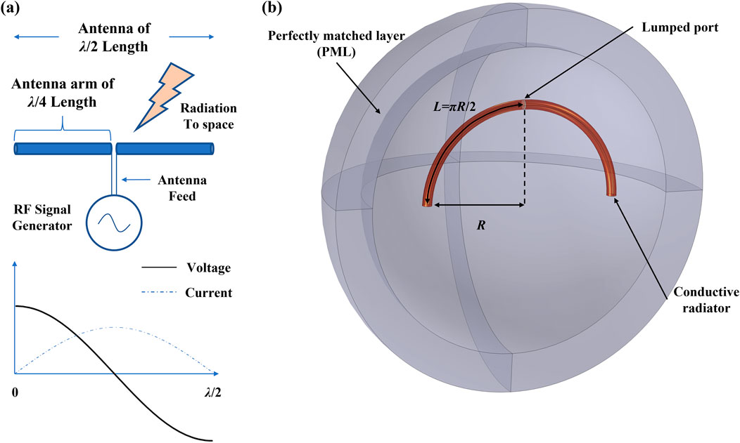
Figure 3. Antenna model. (a) Quarter-wave principle (b) 3D structure.

3.2 Model validation

Taking a typical dipole antenna with radius R = 0.05 m as an example, the relationship between antenna efficiency, power, and return loss (S11, defined as the ratio of the reflected sinusoidal wave amplitude to the incident sinusoidal wave amplitude at port 1) versus operating frequency within the range of 0.5–1.5 GHz was analyzed to validate the model. This high-frequency range targets the antenna’s resonant band, providing the most stringent test of the model’s accuracy in capturing fundamental EM behavior before its application to the low-frequency operational range.

In Figure 4, the orange dashed line indicates the frequency (0.89 GHz) corresponding to the maximum antenna efficiency (η = 0.99). The green dashed line represents the theoretical resonant frequency of the antenna (0.95 GHz), calculated based on the relationship between the speed of light and wavelength (see Equation 8), where the antenna efficiency η = 0.88.

$\mathit{f}=\frac{\mathit{c}}{\mathit{\lambda }}=\frac{\mathit{c}}{4\times \mathit{L}}=\frac{\mathit{c}}{2\mathit{\pi }\mathit{R}}(8)$

where c is the speed of light, λ is the wavelength, L is the antenna arm length, and R is the antenna radius.

Figure 4

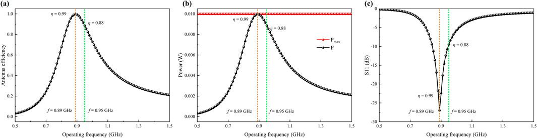
Figure 4. Model validation. (a) Antenna efficiency (b) Power (c) S11.

The results show that the frequencies corresponding to the maximum power ratio and the minimum return loss (S11) coincide with the frequency of maximum antenna efficiency, thereby validating the model. Furthermore, a slight offset is observed between the frequency of maximum efficiency and the theoretical resonant frequency. This phenomenon is attributed to the presence of a diameter size in the antenna of the simulation model, causing the capacitive loading effect at the conductor’s ends to shift the antenna’s theoretical resonant frequency higher.

3.3 Investigation of key factors affecting ED antenna reception efficiency

3.3.1 Influence of operating frequency

The operating frequency range of 0.5–1.5 GHz adopted in the preceding analysis was derived from the relationship between the speed of light and wavelength, targeting proximity to the antenna’s theoretical resonant frequency. Given that deep detection tools typically utilize lower operating frequencies to enhance the DOD, the frequency was set to 6–48 kHz while maintaining a fixed antenna radius R (hence constant arm length L). The relationship between antenna efficiency and frequency under varying surrounding media types (air/formation) was then analyzed to reveal the underlying influence mechanisms of low-frequency variations on antenna reception efficiency.

In Figure 5, the results indicate that when the antenna is situated in an air surrounding medium, its efficiency in the low-frequency band is extremely low. This occurs because the arm length L is significantly shorter than a quarter-wavelength at these frequencies, hindering the formation of an ideal radiation pattern. In contrast, the antenna in the formation surrounding medium demonstrates substantially higher reception efficiency at low frequencies. This reveals that the selection of antenna arm length L in formations is not governed by the quarter-wavelength theory. Moreover, frequency variations exhibit minimal impact on antenna efficiency, whereas formation resistivity emerges as the dominant influencing factor. Consequently, further investigation into the impact of formation resistivity on reception efficiency is necessitated.

Figure 5

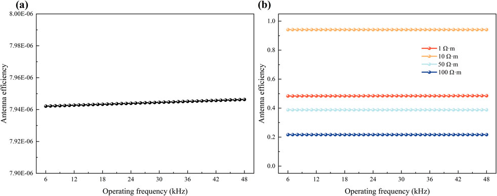
Figure 5. Antenna efficiency as a function of operating frequency under different media. (a) Air (b) Formation.

3.3.2 Influence of formation resistivity

The formation resistivity Rt was set within the range of 1–100 Ω·m, with operating frequencies of 6, 12, 24, and 48 kHz, to analyze the relationship between antenna efficiency and formation resistivity.

In Figure 6, the results demonstrate that at a given operating frequency, antenna efficiency exhibits a non-monotonic trend—initially increasing then decreasing—with rising formation resistivity. This behavior is a direct consequence of impedance matching between the antenna and the coaxial cable. According to the fundamental theory of antenna efficiency (see Equation 5), maximum power transfer and thus peak efficiency occur when the antenna impedance Z matches the characteristic impedance Z_ref of the coaxial cable (set to 50 Ω in this study). As shown in Figure 7, the antenna impedance Z varies with formation resistivity. The resistivity value at which Z approaches 50 Ω corresponds precisely to the peak antenna efficiency observed in Figure 6, confirming that the non-monotonic trend is governed by the impedance matching condition.

Figure 6

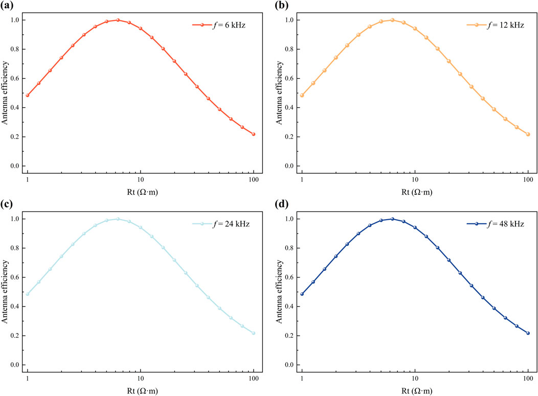
Figure 6. Antenna efficiency as a function of formation resistivity at selected frequencies. (a) f = 6 kHz (b) f = 12 kHz (c) f = 24 kHz (d) f = 48 kHz.

Figure 7

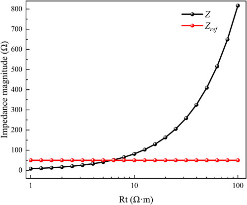
Figure 7. Variation of impedance magnitude with formation resistivity (f = 48 kHz).

In Figure 7, this trend remains remarkably consistent across all tested frequencies, indicating that when the antenna radius R (and thus arm length L) is held constant, formation resistivity serves as the dominant factor governing reception efficiency in subsurface environments. Given that signal response in lossy media is jointly influenced by conductivity and permittivity, the impact of formation relative permittivity on antenna efficiency will be further investigated in the following section.

3.3.3 Influence of relative permittivity

In typical formation environments, the relative permittivity correlates with formation resistivity. Accordingly, the relative permittivity model widely adopted in the petroleum industry (see Equation 9) was applied to the simulations corresponding to Figure 6. With the operating frequency fixed at 48 kHz, the influence of formation relative permittivity on antenna efficiency was analyzed.

$\mathit{\epsilon }=\mathbf{6.4}+\mathbf{4.5255}\sqrt{\mathbf{1}+\sqrt{\mathbf{1}+{\left(\frac{\mathbf{2275}}{\mathbf{\text{Rt}}}\right)}^{\mathbf{2}}}}(9)$

In Figure 8, the results reveal that the impact of relative permittivity on antenna efficiency is negligible. Outcomes obtained with and without considering permittivity effects are virtually identical. This phenomenon occurs because high-frequency signal response in lossy media is significantly affected by permittivity, whereas the low-frequency signals utilized in deep detection tools exhibit minimal sensitivity to permittivity variations. Consequently, the influence of formation relative permittivity can be disregarded.

Figure 8

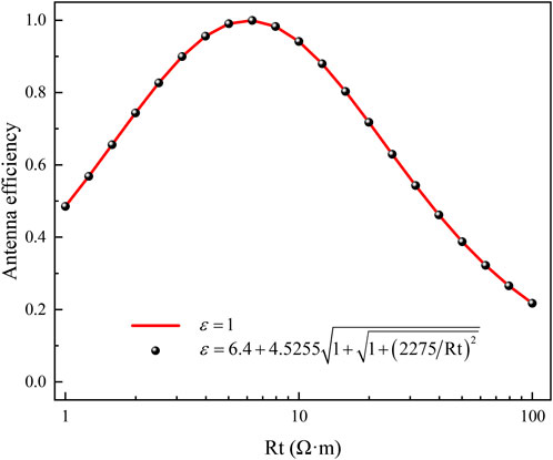
Figure 8. Antenna efficiency as a function of relative permittivity (f = 48 kHz).

3.3.4 Influence of antenna arm length

Previously, the antenna model radius R was consistently set to the conventional value of 0.05 m. To further investigate the influence of antenna arm length L on reception efficiency, the antenna radius (and thus arm length) was adjusted. The antenna performance in air and formation media was compared to elucidate the influence mechanisms of arm length on reception efficiency under different surrounding media conditions.

In Figure 9, the orange dashed line indicates the arm length (0.069 m) corresponding to the maximum antenna efficiency (η = 0.99). The green dashed line represents the theoretical resonant arm length (0.075 m), calculated using the quarter-wavelength theory formula (see Equation 10), where the antenna efficiency η = 0.88. The pink dashed line denotes the antenna efficiency at different formation resistivities when the antenna radius is fixed at 0.05 m.

$\mathit{L}=\frac{\mathit{\lambda }}{\mathbf{4}}=\frac{\mathit{c}}{\mathbf{4}\mathit{f}}(10)$

Figure 9

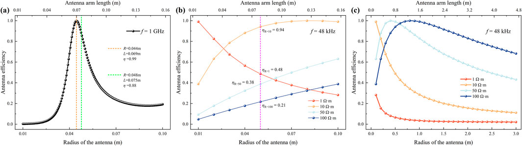
Figure 9. Antenna efficiency as a function of arm length under different media. (a) Air (f = 1 GHz) (b,c) Formation (f = 48 kHz).

The results show that for antennas in an air surrounding medium, reception efficiency initially increases and then decreases with increasing arm length, exhibiting an optimal value. Additionally, the arm length corresponding to maximum efficiency is slightly shorter than the theoretical resonant length. This phenomenon is attributed to the wavelength shortening effect caused by current decay along the symmetric dipole and the end effect. Therefore, an antenna shortening factor (typically 5%) must be introduced when calculating the theoretical resonant arm length. According to Equation 10, achieving high efficiency at low frequencies requires adherence to the quarter-wavelength theory, necessitating increased arm length to form an ideal radiation pattern. In contrast, within formation surrounding media, antennas with radius R = 0.05 m maintain relatively high reception efficiency (0.21–0.94) across different formation resistivities, despite the low operating frequencies.

The above research indicates that the reception efficiency of open-loop half-circle ED antennas cannot be assumed as 100%, unlike closed-loop antennas, and their actual reception efficiency induces attenuation of the tool-received signal. Since ED antenna reception efficiency is governed by the surrounding medium, arm length, and operating frequency, case-specific analysis is imperative. Taking the ED antenna with a standard radius R = 0.05 m (commonly deployed in new deep detection tools) as an example: within formation surrounding media, the influence of operating frequency on reception efficiency is negligible due to low-frequency operation, whereas reception efficiency exhibits a non-monotonic trend—initially increasing then decreasing—with rising formation resistivity. Therefore, efficiency must be quantified based on specific formation resistivity values. When subsequently evaluating the actual boundary detection capability of new deep detection tools, the antenna reception efficiency corresponding to the formation resistivity will be incorporated.

4 Comparative analysis of boundary detection capability

4.1 Azimuthal capability of ED antennas in single-boundary formations

Deep detection tools provide not only formation resistivity measurements but also azimuthal information of formation boundaries. To validate the capability of open-loop half-circle ED antennas in detecting boundary azimuthal information, their azimuthal sensitivity requires further analysis. A single-boundary formation model was constructed, comprising infinitely thick upper and lower layers. The upper layer resistivity R1 = 10 Ω·m, the lower layer resistivity R2 = 1 Ω·m, and the antenna-boundary distance is 1 m.

Figure 10a illustrates the induced EMF variation during 360° tool rotation for both open-loop half-circle ED and tilted closed-loop MD antennas, with 10 m T–R spacing and 48 kHz operating frequency. The results demonstrate that the MD antenna’s EMF follows a cosine-function pattern with 360° periodicity, reaching its maximum at 0° and minimum at 180°. In contrast, while the ED antenna’s EMF also exhibits cosine-like characteristics, it displays 180° periodicity with minima occurring at 90° and 270°. Critically, the ED antenna generates substantially higher EMF amplitude and more pronounced peak-to-peak differential. Given the fundamental periodicity divergence and order-of-magnitude response disparity, direct comparison of boundary identification capability is infeasible. Therefore, azimuthal signals were extracted for quantitative analysis (see Figure 10b).

Figure 10

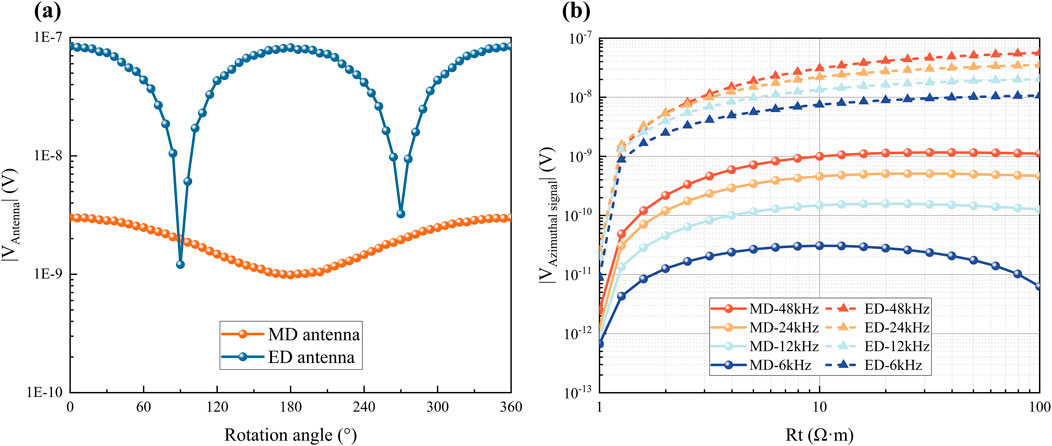
Figure 10. Azimuthal signal analysis. (a) Induced EMF during 360° tool rotation (b) Azimuthal signal response as a function of upper layer resistivity R1.

Figure 10b depicts the azimuthal signal (EMF) response of ED and MD antennas versus upper layer resistivity R1. As R1 increases, both signals exhibit a consistent non-monotonic trend—initially rising then falling—with EMF magnitude scaling positively with frequency. Crucially, the ED antenna demonstrates significantly stronger azimuthal signal intensity and slower attenuation rate. This confirms the open-loop half-circle ED antenna’s superior azimuthal sensitivity, enhanced boundary detection capability, and more effective formation-boundary identification.

The preceding analysis assumed ideal reception efficiency (100%) for the ED antenna. Under actual ED antenna reception efficiency conditions with identical simulation parameters, the azimuthal sensitivity results are shown in Figure 11.

Figure 11

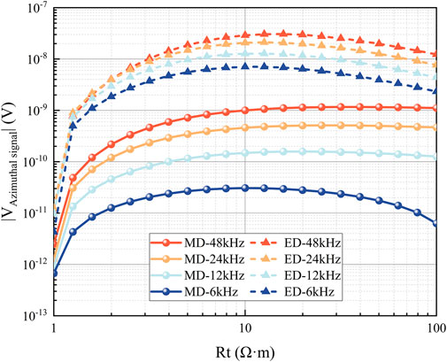
Figure 11. Azimuthal signal response as a function of upper layer resistivity R1 with actual ED antenna reception efficiency.

Figure 11 presents the azimuthal signal (EMF) response of ED and MD antennas versus upper layer resistivity R1, with ED antenna reception efficiency accounted for. The results demonstrate that despite efficiency considerations, the ED antenna’s azimuthal signal strength remains significantly higher than the MD antenna’s-exceeding it by 1-2 orders of magnitude. As R1 increases, the ED antenna’s response pattern aligns with that of the 6 kHz MD antenna, both exhibiting the characteristic non-monotonic trend of initial increase followed by decrease. Although the open-loop half-circle ED antenna shows a slightly higher azimuthal signal attenuation rate compared to 12–48 kHz MD antennas, its superior signal intensity ensures consistently better azimuthal sensitivity than tilted closed-loop MD antennas, enabling more effective formation-boundary identification.

4.2 DOD performance comparison between new and traditional tools

One of the key performance metrics for deep detection tools is their capability to detect formation boundaries, known as the DOD. To compare the DOD between the new and traditional deep detection tools, a horizontally layered two-formation model was constructed. The resistivities across the boundary are R1 and R2, respectively. The tool is positioned within the formation of resistivity R1, with a relative dip angle of 89° to the formation normal. For quantitative DOD assessment, detection thresholds of 0.02 dB for G_Att and 0.05 deg for G_PS were adopted (Yang et al., 2025), as these values are based on the typical signal-to-noise ratio of modern LWD electronics. The distance to boundary (DTB) at which the geosignal magnitude reaches this threshold is defined as the DOD.

The DOD of deep detection tools is strongly dependent on T–R spacing and operating frequency. To visually compare DOD differences between traditional and new tools, simulations determined the maximum achievable DOD across varying T–R spacing and operating frequency through systematic parameter adjustment. The results are presented as 2D maps (also known as the “Picasso Plot”), shown in Figures 12, 13.

Figure 12

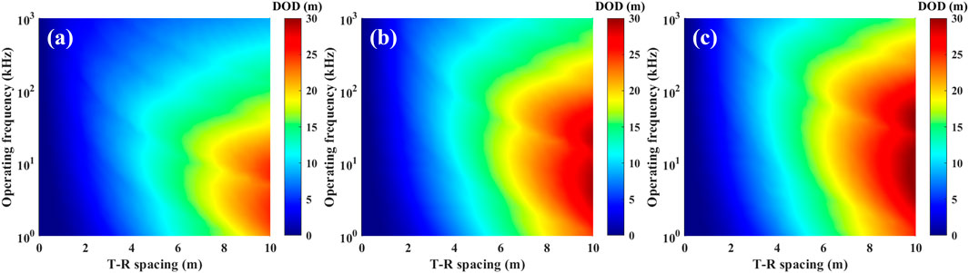
Figure 12. Maximum DOD for traditional deep detection tools under resistivity contrasts. (a) R1:R2 = 10:1 (b) R1:R2 = 50:1 (c) R1:R2 = 100:1.

Figure 13

Figure 13. Maximum DOD for new deep detection tools (ideal efficiency) under resistivity contrasts. (a) R1:R2 = 10:1 (b) R1:R2 = 50:1 (c) R1:R2 = 100:1. The white DOD = 60 m contour is shown for reference.

Figures 12, 13 present the maximum DOD for both traditional and new deep detection tools across varying T–R spacing and operating frequency at resistivity contrasts (R1:R2) of 10:1, 50:1, and 100:1. The results indicate that DOD generally increases with lower operating frequencies; longer T–R spacing extends the detection range while shorter T–R spacing constrains DOD; and lower resistivity in the host formation (i.e., smaller resistivity contrast) reduces DOD. Notably, even at a 10:1 resistivity contrast, the new deep detection tool demonstrates superior performance under short T–R spacing conditions. At identical T–R spacing, the new tool achieves over twice the DOD of the traditional tool. With T–R spacing below 5 m, the new tool readily detects boundaries up to 60 m from the tool, whereas the traditional tool’s maximum DOD is approximately 30 m. To attain equivalent detection ranges, the traditional tool requires T–R spacing several times larger than that of the new tool.

The preceding analysis did not account for the reception efficiency of the ED antenna. When incorporating antenna reception efficiency, the new deep detection tool exhibits antenna efficiencies η of 0.94, 0.38, and 0.21 at formation resistivities R1 of 10 Ω·m, 50 Ω·m, and 100 Ω·m, respectively. Simulations quantified the reduction in maximum DOD (ΔDOD) for the new tool with actual ED antenna reception efficiency by systematically varying T–R spacing and operating frequency. These results are presented in the “Picasso Plot” (see Figure 14), while the actual maximum DOD after accounting for ED antenna reception efficiency is shown in Figure 15.

Figure 14

Figure 14. ΔDOD due to actual ED antenna reception efficiency in new tools. (a) R1:R2 = 10:1 (b) R1:R2 = 50:1 (c) R1:R2 = 100:1.

Figure 15

Figure 15. Actual maximum DOD with actual ED antenna reception efficiency. (a) R1:R2 = 10:1 (b) R1:R2 = 50:1 (c) R1:R2 = 100:1. The white DOD = 60 m contour enables direct comparison with Figure 13.

Figure 14 illustrates the ΔDOD for the new deep detection tool after accounting for ED antenna reception efficiency. The results indicate that the impact of antenna reception efficiency on DOD primarily manifests in the low-frequency band below 100 kHz, with increasingly significant effects at higher resistivity contrasts. The maximum observed ΔDOD exceeds 30 m, attributable to lower antenna efficiency in high-resistivity formations which substantially diminishes the received signal strength, thereby compromising the tool’s boundary detection capability.

Comparative analysis of Figures 12, 13, 15 reveals that without accounting for antenna reception efficiency, the DOD of the new deep detection tool exceeds that of the traditional tool by several-fold. Even when considering antenna reception efficiency effects, the new tool maintains significantly superior DOD performance. Furthermore, the “Picasso Plots” of maximum DOD for the new tool show negligible variation between scenarios assuming ideal efficiency and those incorporating actual ED antenna efficiency. This leads to the conclusion that the new deep detection tool—despite lower ED antenna reception efficiency under high-resistivity conditions (e.g., 100:1 contrast ratio)—demonstrates substantially enhanced boundary detection capability compared to the traditional tool.

5 Conclusion

This study systematically investigates the feasibility of open-loop half-circle ED antennas for boundary detection in LWD AEM, with focused analysis on antenna reception efficiency’s impact on the DOD of new deep detection tools. A comprehensive framework integrating antenna characterization, reception efficiency simulation, and tool DOD evaluation was established. Through comparative analysis of attenuation characteristics between open-loop half-circle ED and traditional closed-loop MD antennas in homogeneous media, azimuthal sensitivity in single-boundary formations, and quantitative DOD assessment of new versus traditional tools, the practical value of ED antennas for LWD boundary detection is conclusively demonstrated.

The primary contribution lies in revealing the governing mechanism of ED antenna reception efficiency. Simulation methods based on the reciprocity theorem establish that formation resistivity dominates reception efficiency when antenna radius R (and thus arm length L) is fixed, while operating frequency and relative permittivity exhibit negligible effects in the low-frequency bands typical for deep detection tools. This finding provides theoretical foundations for accurate signal response evaluation in new deep detection tools, addressing the limitation of assuming 100% antenna reception efficiency in existing studies and offering critical support for optimized tool design and deployment.

The second key contribution resides in clarifying the DOD capability of the new deep detection tool equipped with ED antennas. Comparative analysis confirms that—regardless of whether antenna reception efficiency is considered—the new tool delivers significantly superior DOD performance (exceeding twice that of traditional tools using tilted MD antennas). Even under low-efficiency conditions (e.g., 100 Ω·m formations), the new deep detection tool retains robust boundary detection capability, with particularly enhanced advantages at short T–R spacing (<5 m). This establishes an effective technical approach for long-range formation boundary detection in complex hydrocarbon reservoirs.

Data availability statement

The raw data supporting the conclusions of this article will be made available by the authors, without undue reservation.

Author contributions

CF: Investigation, Methodology, Writing – original draft, Writing – review and editing. ZX: Methodology, Writing – review and editing. HH: Investigation, Writing – review and editing. SD: Methodology, Writing – review and editing. YF: Funding acquisition, Methodology, Writing – review and editing. CQ: Validation, Writing – review and editing. GL: Validation, Writing – review and editing.

Funding

The author(s) declare that financial support was received for the research and/or publication of this article. We are indebted to the financial support from the National Natural Science Foundation of China (No.U23B2086).

Conflict of interest

Authors ZX, HH, CQ and GL were employed by China National Logging Corporation.

The remaining authors declare that the research was conducted in the absence of any commercial or financial relationships that could be construed as a potential conflict of interest.

Generative AI statement

The author(s) declare that no Generative AI was used in the creation of this manuscript.

Any alternative text (alt text) provided alongside figures in this article has been generated by Frontiers with the support of artificial intelligence and reasonable efforts have been made to ensure accuracy, including review by the authors wherever possible. If you identify any issues, please contact us.

Publisher’s note

All claims expressed in this article are solely those of the authors and do not necessarily represent those of their affiliated organizations, or those of the publisher, the editors and the reviewers. Any product that may be evaluated in this article, or claim that may be made by its manufacturer, is not guaranteed or endorsed by the publisher.

References

Bell, C., Hampson, J., Eadsforth, P., Chemali, R., Helgesen, T., Meyer, H., et al. (2006). “Navigating and imaging in complex geology with azimuthal propagation resistivity while drilling,” in SPE Annual Technical Conference and Exhibition. doi:10.2118/102637-MS

CrossRef Full Text | Google Scholar

Bittar, M., Klein, J., Beste, R., Hu, G., Wu, M., Pitcher, J., et al. (2009). A new azimuthal deep-reading resistivity tool for geosteering and advanced formation evaluation. SPE Reserv. Eval. and Eng. 12 (02), 270–279. doi:10.2118/109971-PA

CrossRef Full Text | Google Scholar

Hagiwara, T. (2018). Detection sensitivity and new concept of deep reading look-ahead look around geosteering tool. SEG Int. Expo. Annu. Meet. (1), 714–718. doi:10.1190/segam2018-2981412.1

CrossRef Full Text | Google Scholar

Kang, Z., Wang, H., and Yin, C. (2022a). Finite-region approximation of EM fields in layered biaxial anisotropic media. Remote Sens. 14 (15), 3836. doi:10.3390/rs14153836

CrossRef Full Text | Google Scholar

Kang, Z., Wang, H., and Yin, C. (2022b). Semi-analytic sensitivity of the MCIL responses in homogeneous biaxial anisotropic media. IEEE Geoscience Remote Sens. Lett. 19, 1–5. doi:10.1109/LGRS.2022.3225598

CrossRef Full Text | Google Scholar

Li, S. (2018). System and methodology of look ahead and look around LWD tool. U.S. Pat. WO 2018/052819 A1.

Google Scholar

Liu, Q. Q., Zhuang, M., Zhan, W., Shi, L., and Liu, Q. H. (2023). A hybrid implicit-explicit discontinuous galerkin spectral element time domain (DG-SETD) method for computational elastodynamics. Geophys. J. Int. 234 (3), 1855–1869. doi:10.1093/gji/ggad168

CrossRef Full Text | Google Scholar

Liu, Y., Wang, L., Wang, C., Wang, H., and Qiao, P. (2023). Corrections of logging-while-drilling electromagnetic resistivity logging data acquired from the horizontal well for the shale oil reservoir. Appl. Geophys. 20 (1), 9–19. doi:10.1007/s11770-022-0954-2

CrossRef Full Text | Google Scholar

Luo, K., Zong, Z., Yin, X., Zuo, Y., Fu, Y., and Zhan, W. (2025). Shale pore pressure seismic prediction based on the hydrogen generation and compaction-based rock-physics model and bayesian hamiltonian monte carlo inversion method. Geophysics 90 (2), M15–M30. doi:10.1190/geo2024-0325.1

CrossRef Full Text | Google Scholar

Qiao, P., Wang, L., Yuan, X., and Deng, S. (2024). A new approximation modeling method for the triaxial induction logging in planar-stratified biaxial anisotropic formations. Remote Sens. 16 (16), 3076. doi:10.3390/rs16163076

CrossRef Full Text | Google Scholar

Štumpf, M. (2016). Receiving-antenna Kirchhoff-equivalent circuits and their scattering reciprocity properties. IET Microwaves, Antennas and Propag. 10 (9), 983–990. doi:10.1049/iet-map.2016.0100

CrossRef Full Text | Google Scholar

Wang, L., Li, S., and Fan, Y. (2020). An all-new ultradeep detection method based on hybrid dipole antennas in electromagnetic logging while drilling. IEEE Trans. Geoscience Remote Sens. 58 (3), 2124–2134. doi:10.1109/TGRS.2019.2953304

CrossRef Full Text | Google Scholar

Wang, L., Deng, S., Xie, G., Li, S., Wu, Z., and Fan, Y. (2022). A new deep-reading look-ahead method in electromagnetic logging-while-drilling using the scattered electric field from magnetic dipole antennas. Petroleum Sci. 19 (1), 180–188. doi:10.1016/j.petsci.2021.09.035

CrossRef Full Text | Google Scholar

Wang, L., Cao, F., Li, Z., Yuan, X., and Fan, Y. (2024). A novel propagator coefficient algorithm for modeling induction-type logging responses in cylindrically layered media. IEEE Geoscience Remote Sens. Lett. 21, 1–5. doi:10.1109/LGRS.2024.3401126

CrossRef Full Text | Google Scholar

Wang L., L., Han, Y., Li, Z., Hao, D., and Deng, S. (2025). The joint physics and data-driven geometrical factor of array laterolog in layered formations. Geophysics 90 (1), D11–D25. doi:10.1190/GEO2024-0112.1

CrossRef Full Text | Google Scholar

Wang, Y., Wang, H., Yang, S., Yu, L., Chen, B., Zhang, W., et al. (2025a). Fast 3-D modeling of the LWD ultradeep resistivity measurements using the field-based secondary-field finite volume method. IEEE Trans. Geoscience Remote Sens. 63, 1–16. doi:10.1109/TGRS.2025.3536792

CrossRef Full Text | Google Scholar

Wang, Y., Wang, H., Yu, L., Zhang, W., Liang, P., Chen, W., et al. (2025b). Efficient algorithm of contraction high-order born approximation on LWD ultra-deep resistivity measurement in 3-D anisotropic formation. IEEE Trans. Geoscience Remote Sens. 63, 1–12. doi:10.1109/TGRS.2024.3511666

CrossRef Full Text | Google Scholar

Wu, Z., Li, H., Han, Y., Zhang, R., Zhao, J., and Lai, Q. (2022a). Effects of formation structure on directional electromagnetic logging while drilling measurements. J. Petroleum Sci. Eng. 211, 110118. doi:10.1016/j.petrol.2022.110118

CrossRef Full Text | Google Scholar

Wu, Z., Yue, X., Li, G., Liu, T., and Zhao, J. (2022b). A novel and efficient dimensionality-adaptive scheme for logging-while-drilling electromagnetic measurements modeling. J. Petroleum Sci. Eng. 215, 110572. doi:10.1016/j.petrol.2022.110572

CrossRef Full Text | Google Scholar

Wu, K., Wang, L., Deng, S., and Kou, X. (2025). A novel logging method for detecting highly resistive formations in oil-based mud using high-frequency electrodes. Petroleum Sci. 22 (5), 1946–1958. doi:10.1016/j.petsci.2025.03.010

CrossRef Full Text | Google Scholar

Yang, K., Wang, L., Fang, H., Ai, W., Wang, N., and Zeng, Z. (2025). A new logging-while-drilling azimuthal electromagnetic measurement for highly resistive coal mines. J. Geophys. Eng. 22, 1017–1025. doi:10.1093/jge/gxaf056

CrossRef Full Text | Google Scholar

Zhan, W., Zhuang, M., Liu, Q. Q., Shi, L., Sun, Y., and Liu, Q. H. (2021). Frequency domain spectral element method for modelling poroelastic waves in 3-D anisotropic, heterogeneous and attenuative porous media. Geophys. J. Int. 227 (2), 1339–1353. doi:10.1093/gji/ggab269

CrossRef Full Text | Google Scholar

Zhan, W., Chen, Y., Liu, Q., Li, J., Sacchi, M. D., Zhuang, M., et al. (2024). Simultaneous prediction of petrophysical properties and formation layered thickness from Acoustic logging data using a modular cascading residual neural network (MCARNN) with physical constraints. J. Appl. Geophys. 224, 105362. doi:10.1016/j.jappgeo.2024.105362

CrossRef Full Text | Google Scholar

Zhang, P., Deng, S., Yuan, X., Liu, F., and Xie, W. (2025). Fast forward modeling and response analysis of extra-deep azimuthal resistivity measurements in complex model. Front. Earth Sci. 13, 1506238. doi:10.3389/feart.2025.1506238

CrossRef Full Text | Google Scholar

Zhao, J., Li, W., Xiao, C., Qi, X., and Yuan, S. (2018). Numerical simulation and correction of electrical resistivity logging for different formation dip angles. J. Petroleum Sci. Eng. 164, 344–350. doi:10.1016/j.petrol.2018.01.067

CrossRef Full Text | Google Scholar

Zhao, J., Pei, H., Luo, L., Huang, Y., Wu, Z., and Jia, J. (2025). Anisotropic response characteristics of array induction logging in laminated shale and its correction methods. SPE J. 30 (02), 729–742. doi:10.2118/223961-PA

CrossRef Full Text | Google Scholar