Abstract
Comprehensive and accurate characterization of pore–throat structures is essential for rational resource assessments and enhanced recovery rates in tight sandstone reservoirs. However, the fractal characteristics of full-scale pores and throats in tight sandstones remain poorly understood. In this study, high-pressure mercury intrusion (HPMI), constant-rate mercury intrusion (CRMI), and nuclear magnetic resonance (NMR) experiments are integrated to provide a full-scale characterization of pore and throat distributions in tight sandstone samples. Fractal dimensions are calculated separately for pores and throats using a wetting-phase model and a 3D capillary tube model. Based on these results, seven pore–throat systems are identified: 1) small bundle-like throats within clay interstitial filler, 2) medium tubular/sheet throats generated by intense compaction, 3) large throats formed by localized dilation of tubular/sheet throats, 4) micropores created by localized constriction of submicron–micron sized intergranular pores, 5) small pores dominated by intragranular dissolution pores, 6) medium pores consisting mainly of residual intergranular pores, and 7) large pores resulting from the combination of moldic pores and residual intergranular pores. Moreover, the reservoir space exhibits a ternary structural characteristic. Both small and medium throats conform to the capillary tube assumption, with mean fractal dimensions of 2.2093 and 2.7214, respectively. Small, medium, and large pores fit the spherical assumption, with mean fractal dimensions of 2.8180, 2.7435, and 2.9825, respectively. Extensive overlap between large throats and micropores forms a beaded pore–throat network for which an appropriate fractal model is currently lacking. The porosity and permeability of the samples in this study are primarily controlled by medium pores and medium throats, followed by small pores, while movable fluid resides predominantly within medium pores. The results suggest that relatively weak compaction is a key factor in the development of high-quality reservoirs in the strata studied. The proposed full-scale classification scheme based on fractal dimensions offers new insights into the microscopic heterogeneity of tight sandstones. Furthermore, the full-scale characterization combined with correlation analysis and pore–throat genesis discrimination provides targeted strategies for exploration of high-quality, tight sandstone reservoirs.
1 Introduction
The pore–throat structure is a key factor influencing reservoir storage capacity and flow behavior (Wang J. et al., 2024), and it controls both hydrocarbon occurrence and development efficiency (Dou et al., 2021; Wu Y. et al., 2022; Wang et al., 2024c). In tight sandstone reservoirs, intense diagenesis, particularly compaction, profoundly alters the pore–throat network (Liu et al., 2024; Wang et al., 2024c; Yang Y. et al., 2024), resulting in a broad size distribution (Wang J. et al., 2021; Wu Y. et al., 2022) that is dominated by nano-to micro-scale features (He et al., 2024; Wang J. et al., 2024). This network displays irregular morphology (Wang et al., 2024b), limited connectivity (He et al., 2024; Liu et al., 2024; Wang et al., 2024c; Yang Y. et al., 2024) and pronounced heterogeneity (Wu Y. et al., 2022; He et al., 2024; Liu et al., 2024; Wang et al., 2024c), all of which complicate hydrocarbon grading evaluation (Xie et al., 2023) and impede enhanced recovery rates (Xiao et al., 2016; Xin et al., 2022; Xu et al., 2022; He et al., 2024). Consequently, accurate and comprehensive characterization of pore–throat structure has become a central focus of tight sandstone research worldwide (Xie et al., 2023; He et al., 2024; Wang et al., 2024b). Previous studies have examined pore throats through Euclidean geometry, fractal theory, and topological analysis (Wu et al., 2019). The present work emphasizes fractal characterization grounded in Euclidean representations.
Euclidean geometric descriptors of pore throats encompass their morphology, absolute dimensions, and size-frequency distributions. Currently, two principal categories of characterization techniques have been established: direct methods based on image analysis, represented by scanning electron microscopy (SEM), atomic force microscope (AFM), and X-ray computed tomography (X-CT), and indirect methods based on fluid injection or physical radiation parameter conversion, exemplified by experiments such as high-pressure mercury intrusion (HPMI), constant-rate mercury intrusion (CRMI), nuclear magnetic resonance (NMR), NMR cryoporometry (NMR-C), N2 gas adsorption (N2GA), CO2 gas adsorption (CO2GA) and small-angle x-ray scattering (SAXS) (Wu et al., 2019; Wu Y. et al., 2022; Yang et al., 2023; He et al., 2024; Liu et al., 2024; Wang J. et al., 2024; Wang et al., 2024c; Yang M. et al., 2024; Zhu et al., 2025). No single technique, however, spans the entire nano–micro–milli scale of pore throat diameters (Pan et al., 2021; Qiao et al., 2022; Yang et al., 2023; Wang et al., 2024c), nor can most techniques reliably distinguish pores from throats. Hence, combined approaches that leverage complementary detection ranges and models are increasingly adopted (Qiao et al., 2022; He et al., 2024; Wang et al., 2024b; Wang et al., 2024c). In such schemes, calibrated NMR T2 spectra typically represent pore radius distributions from submicron to millimeter scales (Wu Y. et al., 2022; Liu et al., 2024; Wang et al., 2024c); HPMI, NMR-C, or N2GA resolve nano-scale pore throats (Wu et al., 2019; He et al., 2024); CO2GA and SAXS target ultrafine pore throats (<2 nm) (Wang J. et al., 2024); while discrimination between pores and throats relies on CRMI (Xiao et al., 2016; Wang F. et al., 2021; Wang et al., 2024c; Wu Y. et al., 2022) or high-resolution X-CT (Zhang et al., 2020).
Fractal theory has established the self-similar nature of rock pore–throat systems (Katz and Thompson, 1985; Krohn, 1988), with the fractal dimension (Df) serving as a robust quantitative indicator of microscopic reservoir heterogeneity (Wu Y. et al., 2022; Xu et al., 2022; Zang et al., 2022; Yang et al., 2023; Wang J. et al., 2024; Wang et al., 2024b; Wang et al., 2024c). In recent years, numerous researchers have applied fractal theory to the microscopic study of reservoirs, developing calculation models tailored to various pore–throat characterization techniques (Wang F. et al., 2018; Zhang et al., 2024). Extensive correlation analyses have been conducted between fractal dimensions and rock components (Han et al., 2023), reservoir quality (Cheng et al., 2023; Wang et al., 2024c), and pore–throat parameters (Nan et al., 2023; He et al., 2024; Liu et al., 2025). These efforts have established a conceptual bridge linking pore–throat structure to macroscopic petrophysical properties and sedimentary diagenetic environments. Empirical evidence indicates that fractal behavior varies across scales within pore–throat networks, yielding distinct Df values from the nano-to-millimeter domains (Wang J. et al., 2021; Qiao et al., 2022; Zhao et al., 2023; Wang et al., 2024b). Some scholars have attempted to explain these scale-dependent variations by extending basic geometric models and proposing classification schemes for pore–throat systems. For instance, Zhu et al. (2019) attributed these variations to pore–throat morphology, dividing pore–throat systems into tubular and bead-like types. Wang et al. (2023), by contrast, linked Df differences to the suitability of fractal computation models, classifying pore–throat models as the shuttlecock model and the spiny ball model.
However, conventional methods for deriving fractal dimensions of pore–throat systems in tight sandstones have typically relied on discrete calculations based on isolated experimental datasets (Zhang et al., 2019; Guo et al., 2020; Pan et al., 2021; Qiao et al., 2022; Wang Z. et al., 2020; Wang J. et al., 2021; Wu Y. et al., 2022; Xin et al., 2022; Xu et al., 2022; Zang et al., 2022). Such fragmented methodology often obscures the continuous, scale-dependent nature of pore–throat fractal behavior and limits the ability to capture the full complexity of the system (Wang X. et al., 2018; Guo et al., 2019). Moreover, existing studies have not conducted full-scale fractal analyses that independently quantify pores and throats using geometry-appropriate models while clearly distinguishing between the two (Qiao et al., 2020; Qu et al., 2020; Wang W. et al., 2020).
To address these gaps, this work integrates HPMI, CRMI, and NMR into a continuous, full-scale characterization framework for pore–throat networks in tight sandstones. Fractal dimensions are calculated separately for pores and throats, and pore–throat systems across multiple scales are delineated, thereby providing new insights into microscopic heterogeneity. Finally, by correlating pore–throat genetic types with reservoir quality, the principal controls on reservoir performance are identified.
2 Materials and methods
2.1 Geological setting and samples
A total of 46 core plugs with standard dimensions of 2.54 cm diameter and 5.5 cm length were used in this study. All samples were collected from the Middle Jurassic tight sandstone in a basin of western China, with the sampling area shown in Figure 1A. All cores consist of channel sandstones deposited in a meandering river system (Figure 1B), at burial depths of 1,970–2,600 m. During the Yanshanian tectonic period, the region underwent episodes of uplift and subsidence, leading to limited fracture development. As a result, all samples analyzed in this study are free of natural fractures.
FIGURE 1

Geological overview of the study area. (A) Location of the sampling area and (B) sedimentary facies and tectonic movement characteristics of the target interval.
2.2 Experimental measurements
Figure 2 depicts the experimental workflow applied to each core plug. Two wafers, 0.5 cm and 1.0 cm in thickness, were cut from the plug top; the thinner wafer was processed into casting thin sections (CTS) while the thicker wafer was used for scanning electron microscopy (SEM). The remaining plug was then subjected to non-destructive measurements of porosity, permeability, saturated-state NMR, and high-speed centrifugation (HSC). Following these tests, the plug was bisected into two specimens of approximately 2.5 cm: one for HPMI and the other for CRMI. Because all measurements are from the same original plug, the resulting datasets are fully paired and directly comparable.
FIGURE 2
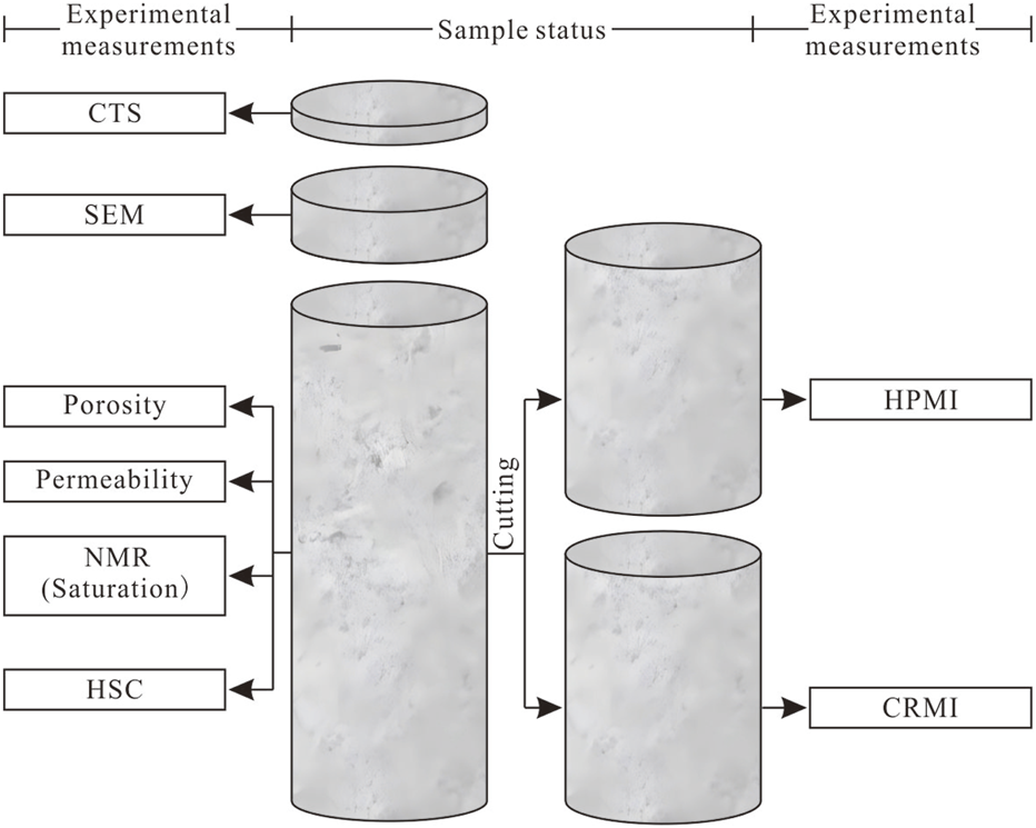
Experimental scheme of single core plug.
2.2.1 CTS and SEM
For CTS analysis, samples were ground to a thickness of approximately 30 μm, impregnated with blue epoxy resin, and examined under a polarizing microscope. During this step, pore morphologies were characterized, genetic classifications determined, and pore radii estimated.
For SEM analysis, samples were fractured, sputter-coated with gold, and imaged using an FEI Quanta-200F field-emission SEM. This procedure emphasized throat morphology and genetic classification, which are features that can be indistinct under optical microscopy, and provided approximate measurements of throat radii.
2.2.2 Porosity and permeability testing
Porosity and permeability were measured using a PoroPDP-200 helium-porosimeter/permeameter (Core Lab, USA). Prior to testing, all core plugs were dried at 110 °C for 24 h to remove residual fluids. Porosity was calculated from helium-expansion measurements using Boyle’s law. Permeability was determined by an unsteady-state gas-flow method and corrected for gas slippage (Klinkenberg effect).
2.2.3 NMR and HSC
Each plug was weighed dry (m0), evacuated under vacuum for 18 h, and subsequently saturated with degassed deionized water under a confining pressure of 20 MPa for 72 h. The saturated weight (m1) was recorded immediately after removal. T2 spectra were acquired at 32 °C using a low-field NMR analyzer (NMRC12-010V, Newmai, China) with echo spacing of 0.1 ms, an echo count of 9,000, and a repetition time of 6,000 ms.
Following NMR measurement, plugs were subjected to high-speed centrifugation at 14,000 rpm (≈6.5 MPa displacement pressure) for 1 h to expel movable fluids; afterward, the post-centrifugation weight (m2) was recorded. Movable water saturation (Swm) was calculated as Equation 1
2.2.4 HPMI and CRMI
Specimens were oven-dried at 110 °C for 24 h to remove residual moisture. HPMI was performed on an AutoPore IV 9505 analyzer (Micromeritics, USA), and CRMI was performed on an ASPE 730 system (Coretest, USA).
Mercury, as a non-wetting fluid, requires external pressure to invade pore–throat constrictions. Assuming cylindrical capillaries, intrusion pressure (Pc) and throat radius (r) obey the Washburn equation (Washburn, 1921):where Pc is in MPa, σ is the surface tension (mN/m), θ is the contact angle (°), and r is the throat radius (µm).
During HPMI, the maximum intrusion pressure reached 412 MPa, with mercury’s contact angle at 140° and surface tension at 480 mN/m, according to Equation 2, it corresponds to a minimum detectable capillary radius of approximately 2 nm. Prior studies show that throat constrictions behave as cylindrical capillaries, whereas pores exhibit considerably larger radii and irregular geometries. As mercury progresses from throats into pores, capillary forces within the larger pores become negligible, producing a pore-shielding effect whereby HPMI-derived size distributions superimpose pore signals onto throat signals, thereby misrepresenting the true pore radii (Yao and Liu, 2012; Xiao et al., 2016; Zhu et al., 2019).
CRMI addresses this by injecting mercury at a constant low rate (0.00005 mL/min), exploiting the pressure differential between the throat and pore entry. In this study, the maximum CRMI pressure of 6.2 MPa corresponds to a minimum detectable throat radius of approximately 120 nm via the Washburn equation (Washburn, 1921). Because CRMI assumes ideal spherical pores, reported pore radii are equivalent-sphere values; when pores are connected to larger throats, the measured volume actually reflects the combined pore–throat networks, leading to overestimated pore radii. Therefore, only CRMI-derived throat radius data are employed in this study.
2.3 Methodology
2.3.1 Conversion between NMR T2 spectrum and radius distribution
NMR arises from the interaction between atomic nuclei and an external magnetic field (Meng et al., 2016). The transverse relaxation time (T2) measured in NMR experiments reflects both the amplitude and rate of relaxation of hydrogen nuclei within pores and throats of different sizes. The overall transverse relaxation rate is the sum of three contributions (Kleinberg and Horsfield, 1990; Coates et al., 1999):where T2 is the transverse relaxation time, ms; T2B is the bulk relaxation time, ms; is the surface relaxivity, μm/ms; S is the pore–throat surface area, μm2; V is the pore–throat volume, μm3; D is the diffusion coefficient, μm2/ms; γ is the gyromagnetic ratio, (T·ms)−1; G is the average magnetic field gradient, 10−4 T/cm; and TE is the echo spacing, ms.
For a rock sample saturated with a single fluid in a homogeneous magnetic field, and with sufficiently short echo spacing, both the bulk term and the diffusion term can be neglected (Kleinberg and Horsfield, 1990; Daigle and Johnson, 2016). Equation 3 then simplifies to
The surface-to-volume ratio (S/V) relates to pore geometry viawhere Fs is a shape factor: it equals 2 for cylindrical capillaries and 3 for spheres. Combining Equations 4, 5 yields
According to Equation 6, T2 is controlled by ρ and the reciprocal of V/S and is directly proportional to the pore–throat radius r. Thus, larger r values correspond to longer T2. In HPMI experiments, mercury initially overcomes lower capillary forces to invade larger pore throats, and subsequently, with increasing pressure, enters progressively smaller pore throats. Consequently, the cumulative summation of the normalized NMR signal in descending order of T2 produces a curve analogous to the capillary curve. By linearly fitting T2 against V/S for each intrusion-saturation step, the can obtained, from which pore–throat radii r can be calculated under either cylindrical or spherical assumptions. The specific surface area S is derived from HPMI data via Equation 7 (Xiao et al., 2016)
2.3.2 Fractal theory and models
Based on the experimental principles of HPMI, CRMI, and NMR, this study characterizes throat radius distributions using HPMI and CRMI data, assuming that throats behave as capillary tubes. Pore radius distributions are obtained from NMR data assuming spherical pores. Accordingly, the fractal models used to calculate fractal dimensions of pores and throats must conform to these geometric assumptions.
According to fractal theory (Mandelbrot et al., 1984), the self-similarity of storage space in tight sandstones is described by the relationship between the number of pore throats and their radii:where N (>r) is the number of pore throats with radius greater than r, dimensionless; rmax is the maximum radius, µm; f(r) is the probability density function of pore–throat radii; Df is the fractal dimension, dimensionless.
2.3.2.1 3D capillary tube model
The 3D capillary tube model assumes that the reservoir’s storage network comprises capillaries of varying radius and length, which is consistent with the morphological assumptions underlying HPMI and CRMI experiments. When computing the fractal dimension using HPMI and CRMI data, the 3D capillary model should therefore be employed. Because mercury preferentially invades larger capillaries, the cumulative intrusion volume can represent the volume of all throats with a radius exceeding r. Thus, the equivalent number of throats with radius >r is given by (Wang et al., 2018):where VHg is the cumulative intrusion volume, µm3, and l is the capillary length, µm. Equation 9 does not yield the actual throat count but the equivalent number of capillaries of radius r required to fill VHg. Combining Equations 8, 9 giveswhere DT is the throat fractal dimension (dimensionless). Equation 10 simplifies to
Li (2010) incorporated the Washburn equation to recast Equation 11 in terms of mercury saturation SHg and capillary pressure Pc:where a is a dimensionless constant. Taking logarithms of Equation 12, yields
Equation 13 describes a linear relationship in double-logarithmic space between mercury saturation SHg and capillary pressure Pc. Hence, the throat fractal dimension computed via the 3D capillary tube model relates to the slope K1 of this regression aswhere K1 is the slope of the fitted line under the 3D capillary tube model.
2.3.2.2 Wetting-phase model
The wetting-phase model applies to experiments using a wetting-phase fluid as the detection medium (Zhang et al., 2017), and it assumes that the rock’s storage space comprises spheres of radius r. In NMR experiments, deionized water serves as the detection medium. When the shape factor (Fs) is set to 3, the model accurately reflects the distribution of spherical pores, aligning with both the medium requirements and model assumptions of the wetting-phase model. Therefore, when calculating the fractal dimension from NMR data, the wetting-phase model should be selected. Because the wetting fluid preferentially occupies the smallest pores, the cumulative volume of pores with radii below r is (Huang et al., 2017):where V (<r) is the volume of pores <r, µm3; and rmin is the minimum pore radius, µm. From Equation 8, the probability density of pore radii is (Huang et al., 2017):where N (<r) is the count of pores <r and DP is the pore fractal dimension. Substituting Equations 15, 16 yields Equation 17.
The total pore volume iswhere rmax is the maximum pore radius, µm. Thus, According to Equation 17, wetting-phase saturation Sw becomes
For rmax≫rmin, Equation 19 simplifies to Equation 20
Then, taking logarithms gives
Equation 21 describes a linear relationship, in double-logarithmic coordinates, between the wetting-phase and r. Accordingly, the pore fractal dimension calculated from the wetting-phase model relates to the slope of the linear regression line as follows:where K2 is the slope of the fitted line under the wetting-phase model.
3 Results
3.1 Petrophysical properties
Table 1 summarizes porosity, permeability, and movable water saturation for all 46 core plugs, which are labeled A1–A46 in descending porosity. Porosity spans 3.32–15.90% (mean 10.04%, median 9.98%), permeability spans 0.002–38.230 mD (mean 2.218 mD, median 0.181 mD), and movable water saturation is 8.84%–70.68% (mean 44.26%, median 50.75%). Figure 3 demonstrates a strong positive correlation between porosity and permeability (R2 = 0.8446) and shows that movable water saturation increases systematically with both porosity and permeability. Given the relatively strong correlations among porosity, permeability, and movable fluid saturation, the reservoirs represented by the samples were classified into four types, primarily based on porosity, in descending order of quality: type I (>13%), type II (10%–13%), type III (7%–10%), and type IV (<7%) (Table 1).
TABLE 1
| Sample | Type | φ (%) | K (mD) | S m (%) | Sample | Type | φ (%) | K (mD) | S m (%) |
|---|---|---|---|---|---|---|---|---|---|
| A1 | Ⅰ | 15.90 | 38.230 | 53.95 | A24 | Ⅲ | 9.92 | 0.183 | 56.93 |
| A2 | Ⅰ | 15.81 | 5.121 | 58.47 | A25 | Ⅲ | 9.73 | 0.085 | 29.00 |
| A3 | Ⅰ | 15.09 | 3.689 | 48.08 | A26 | Ⅲ | 9.58 | 0.308 | 52.95 |
| A4 | Ⅰ | 14.94 | 3.180 | 56.50 | A27 | Ⅲ | 8.95 | 0.057 | 27.40 |
| A5 | Ⅰ | 14.43 | 25.455 | 67.68 | A28 | Ⅲ | 8.64 | 0.055 | 14.65 |
| A6 | Ⅰ | 14.40 | 5.049 | 59.88 | A29 | Ⅲ | 8.58 | 0.092 | 48.12 |
| A7 | Ⅰ | 14.21 | 0.412 | 45.36 | A30 | Ⅲ | 8.53 | 0.117 | 30.43 |
| A8 | Ⅰ | 14.01 | 1.306 | 62.43 | A31 | Ⅲ | 8.24 | 0.092 | 27.98 |
| A9 | Ⅰ | 13.79 | 0.630 | 53.27 | A32 | Ⅲ | 8.15 | 0.051 | 54.70 |
| A10 | Ⅰ | 13.23 | 0.997 | 56.47 | A33 | Ⅲ | 7.89 | 0.036 | 14.78 |
| A11 | Ⅰ | 13.18 | 7.515 | 61.40 | A34 | Ⅲ | 7.77 | 0.107 | 63.03 |
| A12 | Ⅱ | 12.96 | 5.401 | 67.82 | A35 | Ⅲ | 7.49 | 0.031 | 49.42 |
| A13 | Ⅱ | 12.59 | 0.247 | 50.80 | A36 | Ⅲ | 7.46 | 0.031 | 39.39 |
| A14 | Ⅱ | 12.27 | 0.263 | 70.68 | A37 | Ⅲ | 7.27 | 0.055 | 11.21 |
| A15 | Ⅱ | 12.21 | 0.176 | 49.07 | A38 | Ⅲ | 7.25 | 0.036 | 10.54 |
| A16 | Ⅱ | 12.18 | 0.521 | 58.89 | A39 | Ⅳ | 6.87 | 0.029 | 51.64 |
| A17 | Ⅱ | 11.93 | 0.409 | 60.50 | A40 | Ⅳ | 6.45 | 0.020 | 32.77 |
| A18 | Ⅱ | 11.54 | 0.345 | 48.95 | A41 | Ⅳ | 5.73 | 0.018 | 9.72 |
| A19 | Ⅱ | 10.90 | 0.148 | 49.80 | A42 | Ⅳ | 4.67 | 0.009 | 8.84 |
| A20 | Ⅱ | 10.48 | 0.714 | 63.85 | A43 | Ⅳ | 4.57 | 0.053 | 38.54 |
| A21 | Ⅱ | 10.17 | 0.317 | 70.65 | A44 | Ⅳ | 4.52 | 0.002 | 14.32 |
| A22 | Ⅱ | 10.15 | 0.256 | 53.79 | A45 | Ⅳ | 3.95 | 0.009 | 21.84 |
| A23 | Ⅱ | 10.05 | 0.180 | 44.57 | A46 | Ⅳ | 3.32 | 0.003 | 15.04 |
Sample physical parameter statistics.
φ, porosity, K, permeability, Swm, movable fluid saturation.
FIGURE 3

Relationship between porosity, permeability, and movable fluid saturation.
3.2 Pore and throat types
CTS analysis reveals two principal pore types: residual intergranular pores and secondary dissolution pores. Residual intergranular pores persist between framework grains after compaction and cementation, bounded by relatively straight grain margins, with radii of 20–60 µm (Figure 4A). The visual cement content of samples is below 5%, indicating that compaction is the dominant controlling factor for the development of residual intergranular pores. Secondary dissolution pores include intragranular dissolution pores, which are honeycomb-like voids along feldspar cleavage planes, irregular in shape and 5–15 µm in radius (Figure 4B), and larger but rarer moldic pores formed by complete feldspar removal, which may exceed 100 µm in radius and locally interconnect (Figure 4C).
FIGURE 4
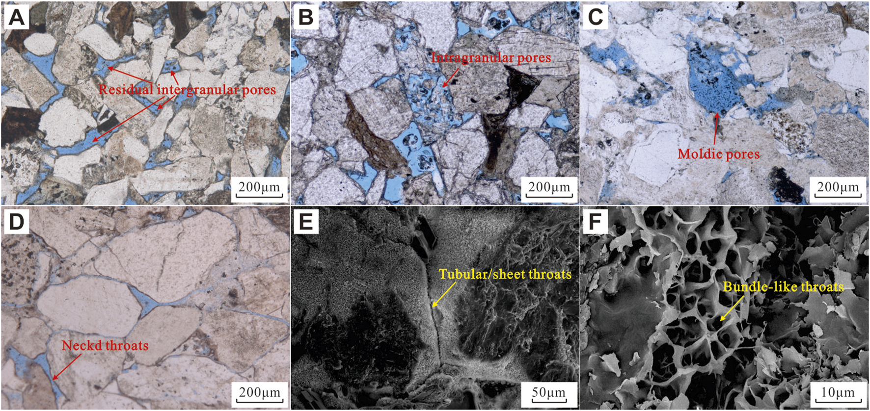
Typical pore and throat types of samples. (A) Residual intergranular pore, sample A8, CTS. (B) Intragranular pore, sample A6, CTS. (C) Moldic pore, sample A21, CTS. (D) Constricted neck-shaped throat, sample 38, CTS. (E) Plate-like throat, sample 31, SEM. (F) Tube bundle throat, sample 29, SEM.
CTS and SEM observations identify three primary throat morphologies: necked, tubular/sheet, and bundle-like. Necked throats result from localized grain-boundary constrictions and measure 1–2 µm in radius (Figure 4D) but occur infrequently. Under strong compaction, tighter grain contacts produce tubular or sheet throats: cylindrical or ellipsoidal throats with radii <1 µm (Figure 4E). Finally, clay interstitial filler domains host abundant bundle-like throats with radii mostly below 0.1 µm (Figure 4F).
3.3 Pore–throat distribution based on single methods
Due to differences in instrument resolution, the raw sampling intervals of HPMI, CRMI, and NMR vary significantly: HPMI yields relatively sparse data points, while CRMI and NMR produce much denser measurements. These discrepancies hinder direct comparison, concatenation, and cross-method computation. To resolve this, CRMI and NMR data were resampled to match the HPMI interval, ensuring that all three techniques generate radius distribution curves with uniform spacing. This standardization enables valid comparison and provides a consistent basis for subsequent curve integration and analysis.
3.3.1 HPMI result
Figures 5A,C,E,G present the capillary pressure curves for each sample. Samples with higher reservoir quality exhibit a broader, gentler plateau at lower mercury saturation and an overall concave-downward shape. As reservoir quality declines, the plateau shortens, the slope steepens, and the curve trends toward a steeper, near-linear form. Final mercury saturations range from 49.64% to 98.44% and do not have a clear correlation with porosity or permeability (Table 2).
FIGURE 5
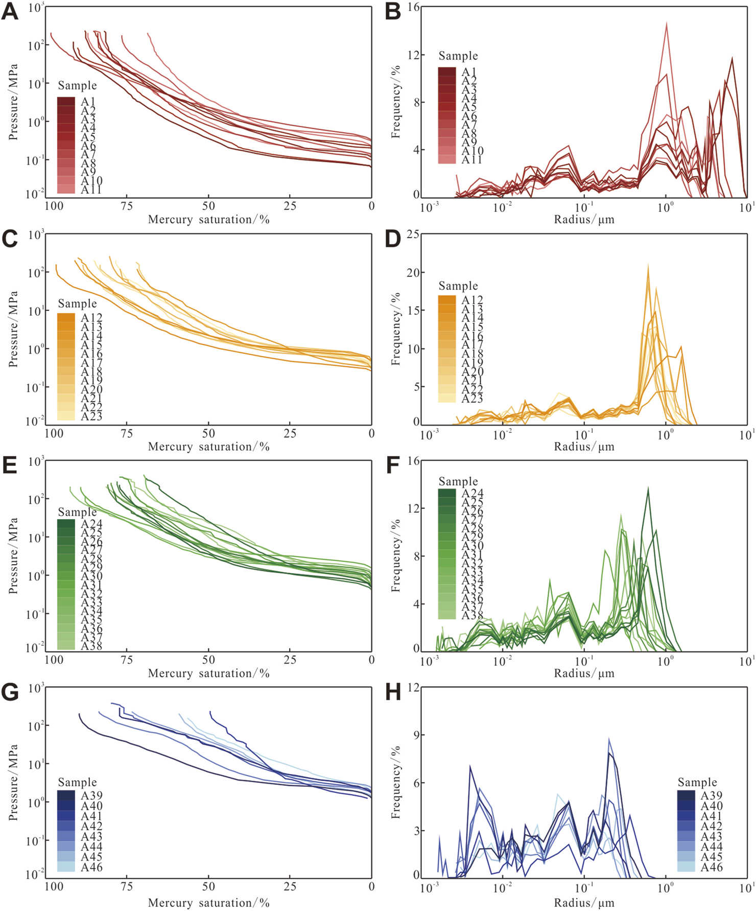
Capillary pressure curve and reservoir space radius distribution of the samples. (A) and (B) Type Ⅰ. (C) and (D) Type II. (E) and (F) Type Ⅲ. (G) and (H) Type Ⅳ.
TABLE 2
| Sample |
r
max
(μm) |
r peak (μm) | r 50 (μm) | (μm) | S Hg (%) | Sample |
r
max
(μm) |
r peak (μm) | r 50 (μm) | (μm) | S Hg (%) |
|---|---|---|---|---|---|---|---|---|---|---|---|
| A1 | 7.555 | 6.479 | 1.822 | 3.043 | 91.39 | A24 | 1.030 | 0.612 | 0.179 | 0.355 | 77.24 |
| A2 | 4.525 | 3.480 | 0.389 | 1.396 | 81.91 | A25 | 0.767 | 0.612 | 0.024 | 0.246 | 69.10 |
| A3 | 3.016 | 0.771 | 0.316 | 0.866 | 87.81 | A26 | 1.031 | 0.765 | 0.158 | 0.363 | 79.03 |
| A4 | 2.388 | 1.890 | 0.496 | 0.921 | 83.93 | A27 | 0.610 | 0.406 | 0.104 | 0.220 | 78.01 |
| A5 | 7.555 | 5.333 | 1.259 | 2.766 | 90.09 | A28 | 0.612 | 0.457 | 0.117 | 0.231 | 80.80 |
| A6 | 5.333 | 4.524 | 0.808 | 1.734 | 85.15 | A29 | 0.508 | 0.284 | 0.117 | 0.191 | 79.95 |
| A7 | 1.611 | 1.032 | 0.265 | 0.414 | 98.44 | A30 | 0.767 | 0.509 | 0.044 | 0.240 | 77.37 |
| A8 | 3.771 | 3.481 | 0.327 | 1.238 | 76.75 | A31 | 0.326 | 0.182 | 0.110 | 0.127 | 89.06 |
| A9 | 1.558 | 1.030 | 0.271 | 0.561 | 85.01 | A32 | 0.768 | 0.285 | 0.208 | 0.233 | 87.92 |
| A10 | 2.409 | 1.030 | 0.170 | 0.759 | 68.63 | A33 | 0.509 | 0.406 | 0.037 | 0.167 | 70.02 |
| A11 | 3.771 | 3.232 | 0.647 | 1.491 | 86.99 | A34 | 0.765 | 0.365 | 0.132 | 0.256 | 74.09 |
| A12 | 2.107 | 1.562 | 0.513 | 0.679 | 96.56 | A35 | 0.509 | 0.284 | 0.176 | 0.187 | 92.38 |
| A13 | 1.023 | 0.762 | 0.270 | 0.365 | 90.89 | A36 | 0.407 | 0.285 | 0.054 | 0.163 | 72.65 |
| A14 | 1.562 | 1.562 | 0.098 | 0.521 | 71.87 | A37 | 0.611 | 0.509 | 0.065 | 0.229 | 81.32 |
| A15 | 0.768 | 0.612 | 0.286 | 0.346 | 90.06 | A38 | 0.767 | 0.509 | 0.026 | 0.363 | 79.03 |
| A16 | 1.564 | 0.768 | 0.180 | 0.464 | 80.21 | A39 | 0.406 | 0.202 | 0.101 | 0.137 | 89.52 |
| A17 | 1.564 | 0.767 | 0.270 | 0.514 | 77.11 | A40 | 0.285 | 0.004 | 0.020 | 0.080 | 77.32 |
| A18 | 1.032 | 0.612 | 0.336 | 0.367 | 88.52 | A41 | 0.509 | 0.365 | — | 0.179 | 49.64 |
| A19 | 1.030 | 0.508 | 0.166 | 0.321 | 83.21 | A42 | 0.285 | 0.202 | 0.019 | 0.085 | 79.80 |
| A20 | 1.032 | 0.767 | 0.169 | 0.394 | 72.31 | A43 | 0.325 | 0.202 | 0.051 | 0.113 | 83.59 |
| A21 | 1.557 | 0.612 | 0.324 | 0.464 | 83.90 | A44 | 0.227 | 0.165 | 0.016 | 0.077 | 73.58 |
| A22 | 1.335 | 0.768 | 0.335 | 0.421 | 85.04 | A45 | 0.365 | 0.285 | 0.014 | 0.121 | 59.09 |
| A23 | 1.033 | 0.766 | 0.128 | 0.376 | 78.39 | A46 | 0.253 | 0.048 | 0.010 | 0.080 | 56.41 |
Pore–throat parameters based on HPMI.
r max, maximum radius; rpeak, peak radius; r50, median radius; , mean radius; SHg, final mercury saturation.
Figures 5B,D,F,H display the pore–throat radius distribution curves based on HPMI, with key size parameters summarized in Table 2. Maximum throat radii range from 0.227 μm to 7.555 μm, peak radii range from 0.004 μm to 6.479 μm, median radii range from 0.010 μm to 1.822 μm, and mean radii range from 0.077 μm to 3.043 μm. As reservoir quality deteriorates, the distributions narrow and shift systematically toward smaller radii.
3.3.2 CRMI result
Figure 6 presents representative capillary pressure curves for pores, throats, and the overall sample. Mercury intrusion proceeds through three distinct stages. In Stage 1 (the “pore stage”), the pore capillary pressure curve coincides with the overall curve, indicating that at low pressure, mercury invades the largest pore bodies first. During this stage, increases in mercury saturation are attributable entirely to pore filling, with no contribution from throats. In Stage 2 (the “pore–throat stage”), the throat capillary pressure curve rises sharply while the pore curve levels off, showing that at intermediate pressures, mercury begins to enter throats and saturation increases are governed primarily by throat filling, even though both pores and throats develop within a relatively narrow range of radii. In Stage 3 (the “throat stage”), the pore capillary pressure curve flattens completely while the throat curve rises slowly, signifying that mercury no longer enters pores but continues to fill throats. All further saturation increases are due to throat invasion, involving only the very small radii.
FIGURE 6
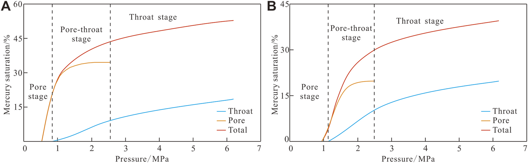
Pore, throat, and total capillary pressure curves of typical samples based on CRMI. (A) Sample A20 and (B) sample A43.
Figure 7 shows the throat radius distribution curves after resampling based on CRMI, with key throat size parameters summarized in Table 3. Maximum throat radii range from 0.325 µm to 4.522 µm, and peak radii range from 0.130 µm to 1.027 µm. Because CRMI is limited in capturing the full throat size spectrum, median and mean throat radii are not reported. As reservoir quality declines, the distributions of throat radius narrow and shift toward smaller values.
FIGURE 7
Throat radius distribution of samples after resampling based on CRMI: (A) Type Ⅰ, (B) Type II, (C) Type Ⅲ, and (D) Type Ⅳ.
TABLE 3
| Sample | r max (μm) | r peak (μm) | Sample | r max (μm) | r peak (μm) |
|---|---|---|---|---|---|
| A1 | 3.772 | 0.769 | A24 | 1.030 | 0.508 |
| A2 | 1.333 | 0.509 | A25 | 0.767 | 0.509 |
| A3 | 2.789 | 0.771 | A26 | 1.031 | 0.767 |
| A4 | 2.112 | 0.613 | A27 | 0.766 | 0.325 |
| A5 | 3.016 | 1.027 | A28 | 0.768 | 0.509 |
| A6 | 1.567 | 0.767 | A29 | 0.764 | 0.284 |
| A7 | 0.766 | 0.509 | A30 | 1.030 | 0.509 |
| A8 | 2.129 | 0.771 | A31 | 0.511 | 0.285 |
| A9 | 1.558 | 0.612 | A32 | 0.768 | 0.130 |
| A10 | 1.332 | 0.612 | A33 | 0.326 | 0.130 |
| A11 | 4.522 | 0.767 | A34 | 0.765 | 0.253 |
| A12 | 2.107 | 0.612 | A35 | 0.766 | 0.509 |
| A13 | 0.762 | 0.507 | A36 | 0.771 | 0.510 |
| A14 | 2.753 | 0.767 | A37 | 1.031 | 0.509 |
| A15 | 0.768 | 0.509 | A38 | 1.337 | 0.767 |
| A16 | 1.030 | 0.284 | A39 | 0.768 | 0.285 |
| A17 | 2.113 | 0.767 | A40 | 0.767 | 0.285 |
| A18 | 0.612 | 0.285 | A41 | 0.611 | 0.365 |
| A19 | 1.030 | 0.130 | A42 | 1.033 | 0.130 |
| A20 | 1.032 | 0.130 | A43 | 0.764 | 0.506 |
| A21 | 1.027 | 0.509 | A44 | 0.325 | 0.227 |
| A22 | 0.768 | 0.285 | A45 | 0.768 | 0.509 |
| A23 | 1.335 | 0.612 | A46 | 0.457 | 0.130 |
Throat-size parameters based on CRMI.
rmax, maximum radius; rpeak, peak radius.
3.3.3 NMR results
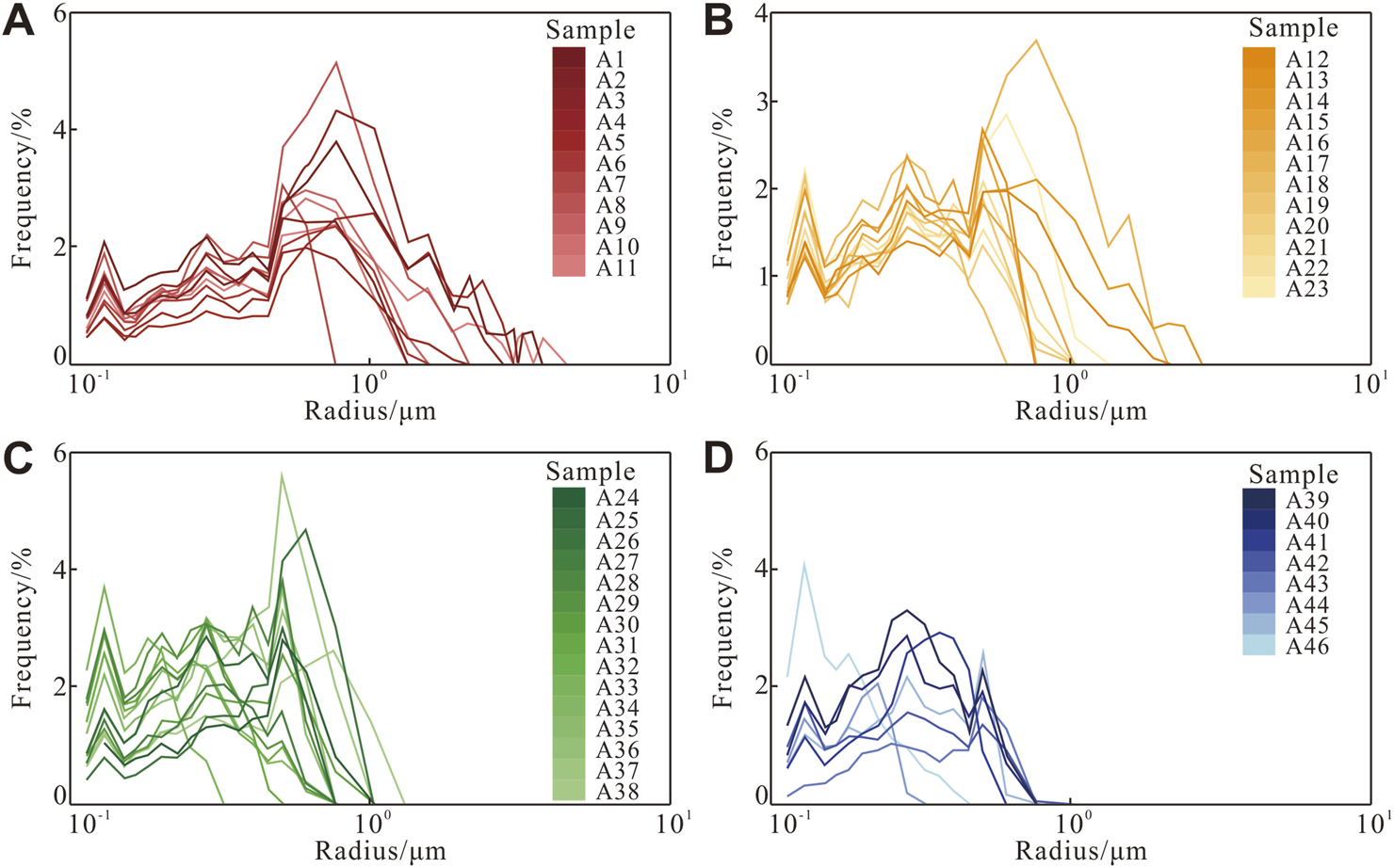
Figures 8A,C,E,G display the NMR T2 spectra for all samples, each exhibiting a bimodal pattern with a dominant short-T2 peak. This short-T2 peak reflects the abundance of small pore throats. As reservoir quality decreases, both the short- and long-T2 peaks shift toward shorter relaxation times, while the short-T2 peak becomes increasingly pronounced, indicating an increasing fraction of small pore throats and an overall reduction in pore throat size.
FIGURE 8
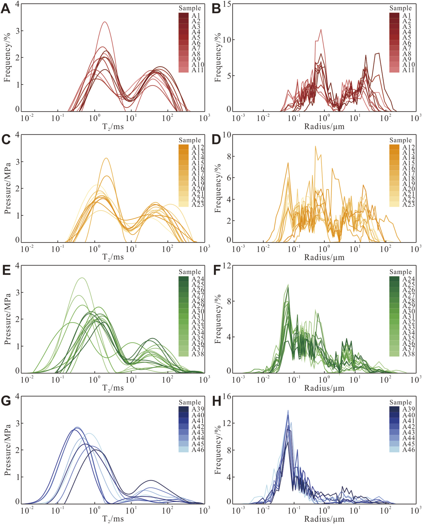
NMR T2 spectra and reservoir space radius distribution after relaxation rate calibration and resampling (Fs = 2). (A) and (B) Type Ⅰ. (C) and (D) Type II. (E) and (F), Type Ⅲ. (G) and (H) Type Ⅳ.
Figures 8B,D,F,H present the corresponding pore–throat radius distribution curves, obtained by calibrating the T2 spectra using surface relaxivity and resampling to match the mercury intrusion interval, with a shape factor of 2 assumed for integration with HPMI and CRMI data. Key parameters are summarized in Table 4: calibrated relaxivities range from 0.039 μm/ms to 0.411 μm/ms; pore–throat radii span minimum values of 0.002–0.227 μm, maximum values of 6.477–218.088 μm, medians of 0.065–11.328 μm, and means of 0.224–23.998 μm. The resampled distributions remain bimodal, with the radii of the left peak at 0.048 μm–1.037 μm and of the right peak at 0.365–60.107 μm. With declining reservoir quality, these distributions progressively shift toward smaller radii.
TABLE 4
| Sample | (μs/ms) |
r
min
(μm) |
r
max
(μm) |
r 50 (μm) | (μm) | Sample | (μs/ms) |
r
min
(μm) |
r
max
(μm) |
r 50 (μm) | (μm) |
|---|---|---|---|---|---|---|---|---|---|---|---|
| A1 | 0.273 | 0.227 | 218.088 | 11.328 | 23.998 | A24 | 0.081 | 0.013 | 113.297 | 0.457 | 3.653 |
| A2 | 0.145 | 0.113 | 45.245 | 1.333 | 7.063 | A25 | 0.092 | 0.015 | 36.305 | 0.202 | 1.287 |
| A3 | 0.107 | 0.048 | 36.261 | 1.035 | 4.854 | A26 | 0.095 | 0.032 | 36.302 | 0.406 | 2.585 |
| A4 | 0.132 | 0.101 | 90.973 | 1.337 | 8.423 | A27 | 0.125 | 0.019 | 113.207 | 0.253 | 1.904 |
| A5 | 0.177 | 0.091 | 147.245 | 6.476 | 15.139 | A28 | 0.113 | 0.002 | 91.010 | 0.285 | 1.746 |
| A6 | 0.137 | 0.065 | 90.973 | 1.030 | 7.456 | A29 | 0.075 | 0.015 | 113.575 | 0.253 | 2.738 |
| A7 | 0.126 | 0.065 | 45.280 | 0.612 | 3.546 | A30 | 0.066 | 0.004 | 146.967 | 0.227 | 2.375 |
| A8 | 0.118 | 0.038 | 59.857 | 1.576 | 5.804 | A31 | 0.061 | 0.019 | 60.060 | 0.182 | 1.381 |
| A9 | 0.154 | 0.130 | 59.903 | 0.767 | 4.737 | A32 | 0.082 | 0.027 | 113.107 | 0.406 | 3.771 |
| A10 | 0.067 | 0.038 | 36.277 | 0.612 | 3.325 | A33 | 0.175 | 0.011 | 217.511 | 0.165 | 2.494 |
| A11 | 0.175 | 0.065 | 174.750 | 3.232 | 10.572 | A34 | 0.059 | 0.027 | 36.276 | 0.325 | 2.659 |
| A12 | 0.135 | 0.065 | 113.581 | 1.885 | 8.512 | A35 | 0.099 | 0.027 | 147.236 | 0.325 | 3.453 |
| A13 | 0.093 | 0.038 | 91.019 | 0.762 | 7.098 | A36 | 0.053 | 0.011 | 36.277 | 0.165 | 1.901 |
| A14 | 0.039 | 0.013 | 45.261 | 0.365 | 2.389 | A37 | 0.411 | 0.019 | 216.900 | 0.284 | 3.026 |
| A15 | 0.094 | 0.027 | 36.299 | 0.509 | 3.220 | A38 | 0.199 | 0.010 | 174.869 | 0.182 | 3.710 |
| A16 | 0.059 | 0.027 | 36.269 | 0.612 | 3.093 | A39 | 0.057 | 0.017 | 113.073 | 0.202 | 3.771 |
| A17 | 0.106 | 0.113 | 45.284 | 0.612 | 4.647 | A40 | 0.052 | 0.005 | 60.018 | 0.091 | 0.849 |
| A18 | 0.096 | 0.038 | 60.026 | 0.769 | 5.048 | A41 | 0.241 | 0.004 | 175.973 | 0.130 | 1.792 |
| A19 | 0.073 | 0.032 | 36.267 | 0.406 | 3.380 | A42 | 0.154 | 0.003 | 113.009 | 0.101 | 1.766 |
| A20 | 0.044 | 0.022 | 36.250 | 0.508 | 3.357 | A43 | 0.063 | 0.011 | 91.261 | 0.151 | 1.882 |
| A21 | 0.054 | 0.032 | 45.259 | 1.888 | 6.523 | A44 | 0.134 | 0.004 | 147.600 | 0.091 | 2.789 |
| A22 | 0.118 | 0.038 | 60.079 | 0.612 | 5.070 | A45 | 0.072 | 0.005 | 60.119 | 0.091 | 1.869 |
| A23 | 0.115 | 0.038 | 45.197 | 0.406 | 3.191 | A46 | 0.044 | 0.004 | 6.477 | 0.065 | 0.224 |
Pore–throat parameters based on NMR T2 spectra calibrated by relaxation rate.
, relaxation rate; rmin, minimum radius; rmax, maximum radius; rpeak-L, peak radius of the left peak; rpeak-R, peak radius of the right peak; r50, median radius; , average radius; SHg, final mercury saturation.
3.4 Full-scale pores and throats distribution based on multiple methods
The HPMI, CRMI, and NMR results for the same sample were plotted on a unified coordinate system (Figures 9A,D,G). The radius distribution curves from the three methods exhibit overlapping peaks, and the left-side shapes of the pore–throat based on HPMI and the throat distributions based on CRMI coincide closely. These agreements confirm both the reliability of the matched HPMI and CRMI data and the accuracy of the NMR relaxivity calibration.
FIGURE 9
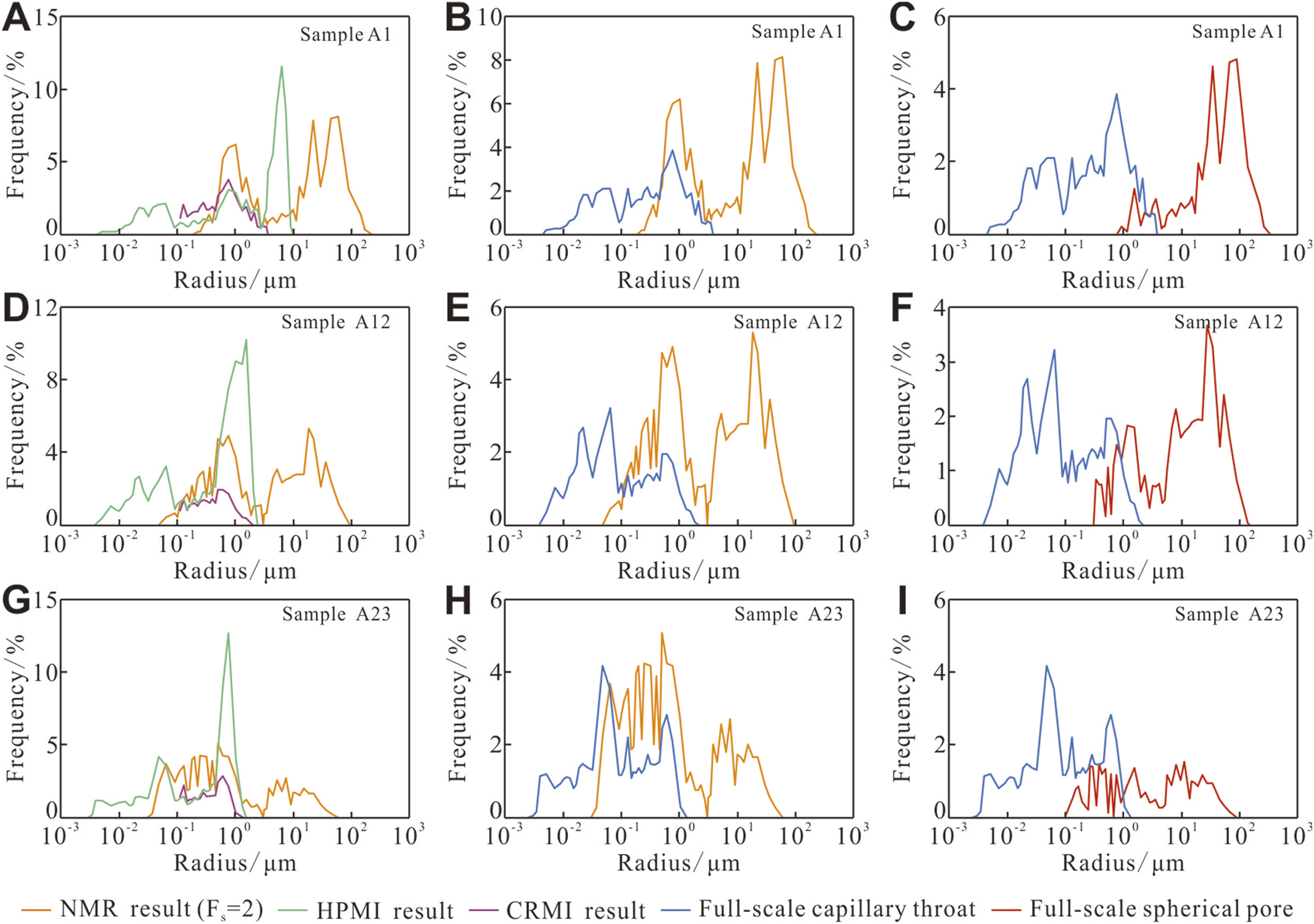
Full-scale capillary throat and spherical pore characterization results of typical samples. (A–C) Sample A1. (D–F) Sample A12. (G–I) Sample A23.
CRMI results demonstrate that only throats occur below a radius of 0.12 μm. Accordingly, in the HPMI distribution, all radii <0.12 μm are attributed to throats. Because both HPMI and CRMI assume capillary tube geometry for throats, their curves can be spliced at 0.12 μm to yield a continuous, full-scale capillary tube throat distribution (Figures 9B,E,H).
The pore–throat distribution based on NMR (with shape factor Fs = 2) can then be directly compared and integrated with this full-scale throat distribution curve. In Figures 8B,E,H, the lower limit of the throat distribution falls below the NMR detection threshold, and in some ranges, the throat proportion exceeds the total pore–throat proportion. This indicates that NMR underrepresents nanometer-scale pore throats because their relaxation times decay too rapidly, faster than the first echo can be sampled. Consequently, only NMR data to the right of the intersection with the full-scale throat curve are used in this study. Subtracting the full-scale throat distribution curve from these NMR data yields the full-scale capillary tube pore distribution, which is then converted to a full-scale spherical pore distribution by multiplying by the geometry conversion factor 3/2 (Figures 9C,F,I).
The main size parameters for the full-scale throats and pores are presented in Tables 5 and 6. Throat radii range from 0.002 μm to 0.009 μm (minimum) to 0.325–3.772 μm (maximum), with median values of 0.020–0.257 μm and mean values of 0.056–0.562 μm. Pore radii satisfy rmax ≫ rmin, with minimum radii of 0.019–0.765 μm, maximum radii of 11.334 μm–624.502 μm, median radii of 0.080–31.670 μm, and mean radii of 0.569–52.871 μm. The pore size characteristics agree well with CTS observations, and the throat-size characteristics align with SEM observations, confirming that the combined HPMI-CRMI-NMR approach provides a realistic description of pore and throat size distributions in tight sandstones.
TABLE 5
| Sample |
r
min
(μm) |
r
max
(μm) |
r 50 (μm) | (μm) | Sample |
r
min
(μm) |
r
max
(μm) |
r 50 (μm) | (μm) |
|---|---|---|---|---|---|---|---|---|---|
| A1 | 0.004 | 3.772 | 0.257 | 0.562 | A24 | 0.002 | 1.030 | 0.087 | 0.188 |
| A2 | 0.002 | 1.333 | 0.147 | 0.255 | A25 | 0.002 | 0.768 | 0.090 | 0.167 |
| A3 | 0.002 | 2.789 | 0.210 | 0.443 | A26 | 0.004 | 1.031 | 0.100 | 0.240 |
| A4 | 0.003 | 2.112 | 0.082 | 0.246 | A27 | 0.002 | 0.766 | 0.056 | 0.139 |
| A5 | 0.005 | 3.016 | 0.195 | 0.552 | A28 | 0.002 | 0.768 | 0.123 | 0.185 |
| A6 | 0.002 | 1.567 | 0.120 | 0.250 | A29 | 0.002 | 0.764 | 0.103 | 0.139 |
| A7 | 0.003 | 0.766 | 0.054 | 0.160 | A30 | 0.002 | 1.030 | 0.050 | 0.149 |
| A8 | 0.003 | 2.130 | 0.255 | 0.387 | A31 | 0.003 | 0.511 | 0.057 | 0.115 |
| A9 | 0.002 | 1.558 | 0.110 | 0.247 | A32 | 0.004 | 0.768 | 0.080 | 0.133 |
| A10 | 0.003 | 1.332 | 0.181 | 0.274 | A33 | 0.002 | 0.326 | 0.047 | 0.083 |
| A11 | 0.003 | 3.4803 | 0.180 | 0.473 | A34 | 0.004 | 0.765 | 0.100 | 0.146 |
| A12 | 0.004 | 2.107 | 0.072 | 0.217 | A35 | 0.003 | 0.766 | 0.099 | 0.167 |
| A13 | 0.003 | 0.762 | 0.062 | 0.167 | A36 | 0.003 | 0.771 | 0.104 | 0.182 |
| A14 | 0.004 | 2.753 | 0.141 | 0.310 | A37 | 0.003 | 1.031 | 0.096 | 0.210 |
| A15 | 0.002 | 0.768 | 0.096 | 0.174 | A38 | 0.002 | 1.337 | 0.034 | 0.168 |
| A16 | 0.002 | 1.030 | 0.057 | 0.166 | A39 | 0.003 | 0.768 | 0.059 | 0.142 |
| A17 | 0.004 | 2.113 | 0.200 | 0.375 | A40 | 0.002 | 0.767 | 0.039 | 0.118 |
| A18 | 0.004 | 0.612 | 0.081 | 0.141 | A41 | 0.002 | 0.611 | 0.119 | 0.174 |
| A19 | 0.004 | 1.030 | 0.045 | 0.143 | A42 | 0.002 | 1.034 | 0.024 | 0.056 |
| A20 | 0.003 | 1.032 | 0.101 | 0.168 | A43 | 0.002 | 0.764 | 0.020 | 0.097 |
| A21 | 0.009 | 1.027 | 0.125 | 0.198 | A44 | 0.002 | 0.325 | 0.020 | 0.058 |
| A22 | 0.003 | 0.768 | 0.050 | 0.147 | A45 | 0.003 | 0.769 | 0.048 | 0.136 |
| A23 | 0.003 | 1.335 | 0.097 | 0.198 | A46 | 0.004 | 0.457 | 0.046 | 0.087 |
Size parameters of full-scale throats.
rmin, minimum radius; rmax, maximum radius; r50, median radius; —average radius.
TABLE 6
| Sample |
r
min
(μm) |
r
max
(μm) |
r 50 (μm) | (μm) | Sample |
r
min
(μm) |
r
max
(μm) |
r 50 (μm) | (μm) |
|---|---|---|---|---|---|---|---|---|---|
| A1 | 0.765 | 624.502 | 31.670 | 52.872 | A24 | 0.057 | 169.945 | 3.710 | 8.190 |
| A2 | 0.303 | 67.868 | 7.536 | 14.214 | A25 | 0.040 | 425.165 | 0.369 | 4.708 |
| A3 | 0.248 | 54.391 | 8.101 | 11.967 | A26 | 0.072 | 220.754 | 1.760 | 5.903 |
| A4 | 0.248 | 425.100 | 7.930 | 17.196 | A27 | 0.057 | 324.022 | 0.642 | 4.676 |
| A5 | 0.170 | 424.286 | 18.207 | 30.709 | A28 | 0.057 | 90.119 | 0.930 | 5.854 |
| A6 | 0.151 | 325.115 | 8.574 | 16.217 | A29 | 0.033 | 170.363 | 1.070 | 7.185 |
| A7 | 0.151 | 67.920 | 1.503 | 7.790 | A30 | 0.057 | 262.113 | 0.608 | 6.447 |
| A8 | 0.072 | 424.389 | 7.038 | 13.372 | A31 | 0.057 | 90.090 | 0.807 | 4.252 |
| A9 | 0.303 | 612.208 | 1.464 | 14.131 | A32 | 0.072 | 169.661 | 3.073 | 7.837 |
| A10 | 0.072 | 261.832 | 4.640 | 7.274 | A33 | 0.057 | 326.267 | 0.459 | 7.926 |
| A11 | 0.136 | 613.064 | 13.728 | 27.615 | A34 | 0.049 | 261.815 | 2.179 | 6.690 |
| A12 | 0.303 | 427.711 | 10.449 | 18.917 | A35 | 0.057 | 263.220 | 2.919 | 9.439 |
| A13 | 0.097 | 263.525 | 6.254 | 16.133 | A36 | 0.033 | 136.381 | 0.675 | 4.207 |
| A14 | 0.033 | 263.305 | 2.776 | 6.358 | A37 | 0.072 | 325.350 | 0.349 | 11.876 |
| A15 | 0.151 | 54.448 | 1.902 | 7.397 | A38 | 0.057 | 262.304 | 0.287 | 9.474 |
| A16 | 0.072 | 262.807 | 4.448 | 7.501 | A39 | 0.057 | 169.609 | 1.762 | 6.429 |
| A17 | 0.272 | 430.136 | 4.725 | 10.902 | A40 | 0.028 | 90.028 | 0.173 | 2.391 |
| A18 | 0.136 | 324.998 | 5.457 | 11.041 | A41 | 0.026 | 263.959 | 0.171 | 3.808 |
| A19 | 0.072 | 169.584 | 3.568 | 7.748 | A42 | 0.040 | 169.514 | 0.176 | 4.922 |
| A20 | 0.040 | 136.148 | 3.321 | 7.193 | A43 | 0.033 | 136.892 | 0.265 | 4.324 |
| A21 | 0.072 | 67.888 | 7.628 | 13.780 | A44 | 0.028 | 263.915 | 0.158 | 7.626 |
| A22 | 0.072 | 423.953 | 4.497 | 11.803 | A45 | 0.028 | 90.178 | 0.172 | 4.190 |
| A23 | 0.097 | 262.043 | 2.250 | 9.442 | A46 | 0.019 | 11.334 | 0.080 | 0.569 |
Size parameters of full-scale pores.
rmin, minimum radius; rmax, maximum radius; r50, median radius; , average radius.
3.5 Full-scale fractal characteristics of pores and throats
The fractal dimensions of throats were calculated using the 3D capillary tube model (Equations 13 and 14). In double-logarithmic plots of lg Pc versus lg SHg, the regression curves exhibit three distinct segments at the slope changes, partitioning the throat network into small, medium, and large throats (Figures 10A–C). Pore fractal dimensions were derived from the wetting-phase model (Equation 22). Similarly, four segments appear in plots of lg r versus lg Sw, delineating micropores, small pores, medium pores, and large pores (Figures 10D–F).
FIGURE 10
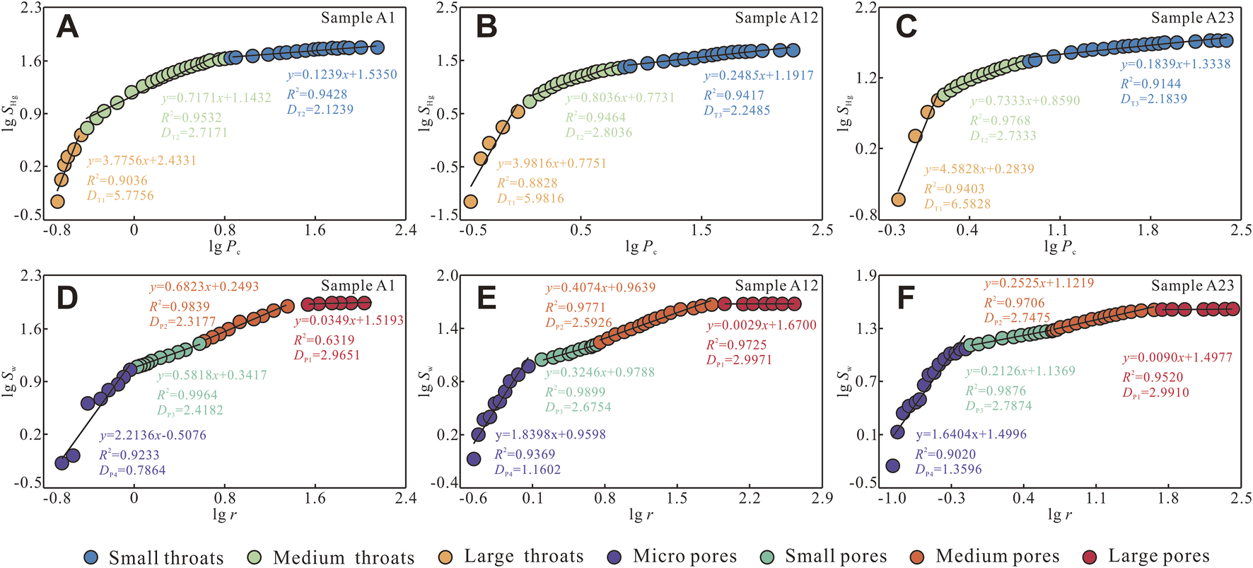
(A–C) Full-scale throat fractal characteristics of samples A1, A12, and A23 (D–F). Full-scale pore fractal characteristics of samples A1, A12, and A23.
The fractal dimensions for each class are listed in Table 7 (throats) and Table 8 (pores), with the corresponding radius ranges shown in Figure 11. In double-logarithmic space, the coefficients of determination for the throat types range from 0.8202 to 0.9917, and for the pore types from 0.8049 to 0.9985, most exceeding 0.9000, demonstrating robust classification. Small throats, with radii of 0.002 μm–0.122 μm (predominantly <0.100 μm), exhibit fractal dimensions DT1 between 2.1168 and 2.3923 (mean 2.2093). Medium throats span 0.100–2.299 μm (mainly 0.100–0.560 μm) and have DT2 between 2.4098 and 2.9393 (mean 2.7214). Large throats range from 0.140 μm to 3.772 μm (mostly 0.345–1.300 μm) with DT3 between 4.8913 and 9.5803 (mean 6.2768). Micropores extend from 0.019 μm to 3.961 μm (predominantly 0.030–1.000 μm) and yield DP1 between 0.2040 and 1.9816 (mean 1.3778). Small pores (1.000–5.430 μm) have DP2 between 2.4182 and 2.9902.
TABLE 7
| Sample | D T1 | R2 | D T2 | R2 | D T3 | R2 | Sample | D T1 | R2 | D T2 | R2 | D T3 | R2 |
|---|---|---|---|---|---|---|---|---|---|---|---|---|---|
| A1 | 2.1239 | 0.9428 | 2.7171 | 0.9532 | 5.7756 | 0.9036 | A24 | 2.1946 | 0.9548 | 2.6571 | 0.9651 | 6.2978 | 0.9669 |
| A2 | 2.1324 | 0.8407 | 2.6714 | 0.9518 | 4.8913 | 0.9848 | A25 | 2.1642 | 0.978 | 2.687 | 0.9333 | 5.6649 | 0.9599 |
| A3 | 2.117 | 0.8737 | 2.5349 | 0.9361 | 6.5113 | 0.9234 | A26 | 2.2175 | 0.9484 | 2.4098 | 0.9062 | 5.3761 | 0.9749 |
| A4 | 2.2042 | 0.8758 | 2.6469 | 0.927 | 6.0948 | 0.9056 | A27 | 2.2046 | 0.9226 | 2.6614 | 0.962 | 6.8577 | 0.9152 |
| A5 | 2.231 | 0.9737 | 2.4828 | 0.912 | 6.7934 | 0.9468 | A28 | 2.1395 | 0.9112 | 2.8137 | 0.9626 | 7.0865 | 0.9588 |
| A6 | 2.1674 | 0.9195 | 2.6832 | 0.9396 | 7.6002 | 0.9139 | A29 | 2.1833 | 0.9709 | 2.8935 | 0.9657 | 6.1252 | 0.9318 |
| A7 | 2.2391 | 0.8971 | 2.6827 | 0.9217 | 5.9254 | 0.9864 | A30 | 2.1879 | 0.8545 | 2.7548 | 0.9311 | 6.7758 | 0.9764 |
| A8 | 2.1223 | 0.9581 | 2.5026 | 0.9335 | 5.2182 | 0.9419 | A31 | 2.2334 | 0.9096 | 2.9255 | 0.9727 | 7.9443 | 0.8805 |
| A9 | 2.1599 | 0.9021 | 2.6007 | 0.9543 | 5.5856 | 0.9399 | A32 | 2.2549 | 0.9758 | 2.9339 | 0.9654 | 6.0437 | 0.9144 |
| A10 | 2.1168 | 0.9215 | 2.6675 | 0.9556 | 5.3681 | 0.9831 | A33 | 2.1906 | 0.827 | 2.9393 | 0.9675 | 6.5574 | 0.9621 |
| A11 | 2.16 | 0.9594 | 2.7161 | 0.9508 | 5.1389 | 0.918 | A34 | 2.2268 | 0.958 | 2.8242 | 0.9769 | 5.6667 | 0.9688 |
| A12 | 2.2485 | 0.9417 | 2.8036 | 0.9464 | 5.9816 | 0.8828 | A35 | 2.1937 | 0.9513 | 2.7401 | 0.9624 | 6.4343 | 0.9205 |
| A13 | 2.2146 | 0.9471 | 2.6431 | 0.9445 | 5.4143 | 0.9682 | A36 | 2.2003 | 0.9526 | 2.5953 | 0.9409 | 5.5594 | 0.9675 |
| A14 | 2.1887 | 0.958 | 2.8503 | 0.9653 | 5.2473 | 0.9585 | A37 | 2.2107 | 0.9835 | 2.4617 | 0.9056 | 5.9371 | 0.9053 |
| A15 | 2.1678 | 0.9421 | 2.7608 | 0.9323 | 5.7199 | 0.9721 | A38 | 2.2498 | 0.9372 | 2.6751 | 0.9548 | 4.9328 | 0.979 |
| A16 | 2.2043 | 0.8974 | 2.8539 | 0.9289 | 5.2762 | 0.9917 | A39 | 2.2289 | 0.9328 | 2.742 | 0.9446 | 6.0805 | 0.9479 |
| A17 | 2.1493 | 0.9699 | 2.5678 | 0.9437 | 6.2835 | 0.8828 | A40 | 2.2565 | 0.9757 | 2.9071 | 0.9266 | 6.6774 | 0.9531 |
| A18 | 2.2334 | 0.9517 | 2.805 | 0.9573 | 6.5475 | 0.9464 | A41 | 2.1711 | 0.9822 | 2.4949 | 0.9518 | 7.4992 | 0.9076 |
| A19 | 2.2994 | 0.9691 | 2.695 | 0.9737 | 7.0082 | 0.9257 | A42 | 2.2786 | 0.9595 | 2.8571 | 0.9748 | 7.8953 | 0.8803 |
| A20 | 2.1728 | 0.9093 | 2.8411 | 0.9756 | 6.0742 | 0.9551 | A43 | 2.37 | 0.9836 | 2.7322 | 0.9216 | 6.0878 | 0.9774 |
| A21 | 2.2425 | 0.9509 | 2.7587 | 0.9597 | 6.2079 | 0.9706 | A44 | 2.3923 | 0.97 | 2.9036 | 0.9672 | 9.5803 | 0.8399 |
| A22 | 2.245 | 0.9725 | 2.7606 | 0.9526 | 5.5897 | 0.9746 | A45 | 2.2532 | 0.9409 | 2.7601 | 0.9393 | 8.9852 | 0.8202 |
| A23 | 2.1839 | 0.9144 | 2.7333 | 0.9768 | 6.5828 | 0.9403 | A46 | 2.3003 | 0.9408 | 2.8378 | 0.9657 | 5.8324 | 0.953 |
Multi-scale fractal dimension of the throat system.
D T1, fractal dimension of small throat; DT2, fractal dimension of medium throat; DT3, fractal dimension of large throat.
TABLE 8
| Sample | D P1 | R2 | D P2 | R2 | D P3 | R2 | D P4 | R2 | Sample | D P1 | R2 | D P2 | R2 | D P3 | R2 | D P4 | R2 |
|---|---|---|---|---|---|---|---|---|---|---|---|---|---|---|---|---|---|
| A1 | 0.7864 | 0.9233 | 2.4182 | 0.9964 | 2.3177 | 0.9839 | 2.9651 | 0.8319 | A24 | 1.298 | 0.9623 | 2.7982 | 0.9811 | 2.6921 | 0.9469 | 2.9879 | 0.9530 |
| A2 | 0.8010 | 0.8913 | 2.7962 | 0.9876 | 2.5919 | 0.9919 | 2.8701 | 0.9607 | A25 | 0.9085 | 0.8178 | 2.8795 | 0.8953 | 2.8422 | 0.9746 | 2.9946 | 0.9665 |
| A3 | 0.6201 | 0.9163 | 2.6857 | 0.955 | 2.4468 | 0.9939 | 2.9397 | 0.9451 | A26 | 1.1471 | 0.9469 | 2.7625 | 0.9797 | 2.7398 | 0.9635 | 2.9962 | 0.9482 |
| A4 | 0.9116 | 0.9106 | 2.8201 | 0.9765 | 2.6580 | 0.9842 | 2.9982 | 0.9586 | A27 | 1.7693 | 0.8873 | 2.8994 | 0.9917 | 2.9066 | 0.9866 | 2.9943 | 0.9032 |
| A5 | 0.3999 | 0.9336 | 2.7657 | 0.9723 | 2.5321 | 0.9647 | 2.9985 | 0.9155 | A28 | 2.0055 | 0.9409 | 2.9147 | 0.9606 | 2.9061 | 0.9883 | 2.9635 | 0.9118 |
| A6 | 1.1305 | 0.9310 | 2.8887 | 0.9468 | 2.6401 | 0.9791 | 2.9961 | 0.9891 | A29 | 1.8059 | 0.8454 | 2.8429 | 0.9742 | 2.7781 | 0.9673 | 2.9785 | 0.8818 |
| A7 | 1.7007 | 0.9146 | 2.8372 | 0.9787 | 2.7542 | 0.9985 | 2.964 | 0.9189 | A30 | 1.9816 | 0.9269 | 2.8345 | 0.9928 | 2.8244 | 0.9465 | 2.9848 | 0.9231 |
| A8 | 1.7962 | 0.9123 | 2.8194 | 0.9216 | 2.5894 | 0.9576 | 2.9958 | 0.9831 | A31 | 1.9715 | 0.8655 | 2.8050 | 0.9722 | 2.8161 | 0.9508 | 2.9900 | 0.9650 |
| A9 | 0.7746 | 0.8534 | 2.9892 | 0.8496 | 2.7496 | 0.9538 | 2.9916 | 0.9402 | A32 | 1.8681 | 0.9269 | 2.7070 | 0.991 | 2.7050 | 0.9480 | 2.9801 | 0.9169 |
| A10 | 0.5813 | 0.9137 | 2.7779 | 0.9430 | 2.6774 | 0.9491 | 2.9982 | 0.9501 | A33 | 2.0289 | 0.9401 | 2.9883 | 0.8799 | 2.9399 | 0.9933 | 2.9893 | 0.9552 |
| A11 | 0.8786 | 0.9101 | 2.7475 | 0.9620 | 2.5232 | 0.9424 | 2.9916 | 0.8773 | A34 | 1.8349 | 0.8171 | 2.8007 | 0.9843 | 2.7429 | 0.9782 | 2.9958 | 0.9540 |
| A12 | 1.1602 | 0.9369 | 2.6754 | 0.9899 | 2.5926 | 0.9771 | 2.9971 | 0.9725 | A35 | 1.8800 | 0.8426 | 2.7573 | 0.9967 | 2.7872 | 0.9371 | 2.9915 | 0.9296 |
| A13 | 1.6408 | 0.8381 | 2.7362 | 0.9910 | 2.7120 | 0.9839 | 2.997 | 0.8892 | A36 | 1.9038 | 0.8930 | 2.8494 | 0.9867 | 2.8191 | 0.9616 | 2.9963 | 0.9019 |
| A14 | 1.6606 | 0.8054 | 2.7920 | 0.9829 | 2.7409 | 0.9360 | 2.9978 | 0.8222 | A37 | 1.8308 | 0.8416 | 2.9768 | 0.8200 | 2.9417 | 0.9927 | 2.9818 | 0.9774 |
| A15 | 1.2036 | 0.9570 | 2.8605 | 0.9911 | 2.6979 | 0.9922 | 2.9785 | 0.8990 | A38 | 1.8674 | 0.8914 | 2.9426 | 0.8441 | 2.9270 | 0.9846 | 2.9803 | 0.9322 |
| A16 | 1.2854 | 0.9408 | 2.7203 | 0.9907 | 2.6372 | 0.9554 | 2.9955 | 0.9566 | A39 | 2.0287 | 0.9392 | 2.7664 | 0.9910 | 2.7779 | 0.9507 | 2.9862 | 0.8949 |
| A17 | 0.2040 | 0.9033 | 2.8923 | 0.8672 | 2.6953 | 0.9589 | 2.9953 | 0.9667 | A40 | 1.6025 | 0.8518 | 2.6911 | 0.9956 | 2.9203 | 0.9934 | 2.9765 | 0.9527 |
| A18 | 1.5809 | 0.8891 | 2.8061 | 0.9828 | 2.6888 | 0.9537 | 2.9988 | 0.9801 | A41 | 1.8604 | 0.8221 | 2.9836 | 0.8561 | 2.9594 | 0.9695 | 2.9863 | 0.9671 |
| A19 | 1.4639 | 0.9645 | 2.7362 | 0.9867 | 2.6876 | 0.9752 | 2.9971 | 0.9424 | A42 | 2.2129 | 0.8283 | 2.9902 | 0.8596 | 2.9608 | 0.9948 | 2.9933 | 0.9981 |
| A20 | 1.2600 | 0.9320 | 2.7252 | 0.9966 | 2.6823 | 0.9719 | 2.9983 | 0.8676 | A43 | 1.9311 | 0.8324 | 2.9246 | 0.9593 | 2.8691 | 0.9695 | 2.9885 | 0.9241 |
| A21 | 0.7506 | 0.9137 | 2.5771 | 0.9839 | 2.5018 | 0.9958 | 2.8865 | 0.9658 | A44 | 1.6032 | 0.8367 | 2.9849 | 0.8193 | 2.9661 | 0.9633 | 2.9942 | 0.9873 |
| A22 | 1.7660 | 0.9528 | 2.8445 | 0.9908 | 2.7357 | 0.9621 | 2.9952 | 0.9593 | A45 | 1.7394 | 0.8136 | 2.8816 | 0.8750 | 2.8662 | 0.9700 | 2.9423 | 0.9721 |
| A23 | 1.3596 | 0.9020 | 2.7874 | 0.9876 | 2.7475 | 0.9706 | 2.991 | 0.9520 | A46 | 1.3465 | 0.8049 | 2.9468 | 0.9838 | 2.9119 | 0.9920 | 2.9846 | 0.8559 |
Full-scale fractal dimension of the pore system.
D P1, fractal dimension of micropores; DP2, fractal dimension of small pores; DP3, fractal dimension of medium pores; DP4, fractal dimension of large pores (mean 2.8180). Medium pores (1.000–5.430 μm) have DP3 between 2.3177 and 2.9661 (mean 2.7435), and large pores (1.000–5.430 μm) exhibit DP4 between 2.8701 and 2.9988 (mean 2.9825).
FIGURE 11

(A) Size distribution range of the throat system. (B) Size distribution range of the pore system.
In three dimensions, true fractal dimensions should lie between 2 and 3 (Zhang et al., 2017), with values closer to 2 indicating lower structural complexity and those closer to 3 reflecting higher complexity. The elevated DT3 for large throats and the low DP1 for micropores deviate from ideal fractal behavior. Notably, some DT3 significantly exceed the upper limit of 3, with maximum values approaching 10. Similarly, some DP1 fall far below 2, with maximum values approaching 0. These physically unrealistic values arise from the presence of throats with relatively large size but very low proportion and pores with relatively small size and significantly lower proportion within the samples. Such characteristics steepen the regression slope for data points corresponding to large throats and micropores. This pattern highlights pronounced heterogeneity in the development of large throats and micropores. Moreover, among throats, DT1 < DT2 indicates that medium throats are more complex than small ones; among pores, DP3 < DP2 < DP4 shows that large pores are most complex, followed by small pores, with medium pores the least complex.
4 Discussion
4.1 Genetic types and ternary structure of pore–throat systems
According to fractal theory, the fractal dimension of a reservoir pore–throat network reflects its geometric scaling: values near 2 correspond to two-dimensional proportional scaling, while those near 3 indicate three-dimensional proportional scaling (Li and Horne, 2006; Zhu et al., 2019; Wang et al., 2023). Dimensions below 2 or above 3 signify a significant departure from the assumed geometry: either a loss of self-similarity or the breakdown of the model.
For the capillary model of throats, the fractal dimension reflects how radius r and length l scale spatially. If r expands equally along two perpendicular axes, or if r and l both extend along a single axis with the same proportion, the throat undergoes two-dimensional proportional scaling (Df = 2). When r and l scale equally in all three dimensions, the throat exhibits three-dimensional proportional scaling (Df = 3) (Figure 12A). Intermediate or more complex scaling behaviors yield fractal dimensions between 2 and 3. Throughout these processes, throats remain cylindrical or ellipsoidal, preserving the capillary tube assumption. However, if throats interweave with adjacent pore bodies and undergo localized widening, their volume increases faster than predicted by the ideal model, and the fractal dimension exceeds 3.
FIGURE 12
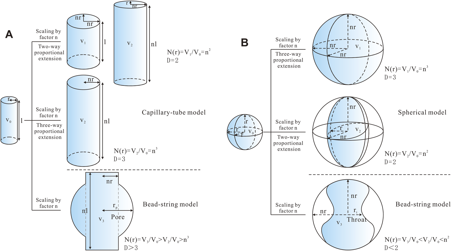
Extended model of reservoir space. (A) Capillary tube model of throat (modified from Zhu et al., 2019), and (B) Spherical model of pores.
For the spherical model of pores, the fractal dimension reflects how the pore radius r scales in three-dimensional space. When r expands equally along all three axes, the pore undergoes three-dimensional proportional scaling (Df = 3); if r expands equally along only two axes, the pore exhibits two-dimensional proportional scaling (Df = 2) (Figure 12B). More complex or intermediate scaling behaviors yield Df values between 2 and 3. Throughout these processes, pore shapes remain roughly spherical or ellipsoidal, justifying the spherical pore assumption. However, if pores interpenetrate throats and undergo local necking, their volume contracts rapidly, causing the fractal dimension to drop below 2.
The radius distribution curves (Figure 11) reveal substantial size overlap between large throats and micropores. In this overlapping range, pores and throats interweave to form a beaded structure that is neither purely spherical nor strictly a capillary tube in geometry. Conventional techniques reliably distinguish large pores at the upper end and small throats at the lower end of the spectrum, but resolution diminishes where pore and throat sizes coincide. As a result, the 3D capillary tube model tends to overestimate fractal dimensions for large throats (Df > 3), while the wetting-phase model underestimates fractal dimensions for micropores (Df < 2).
Figure 13 illustrates the microfeatures and genetic origins of each pore–throat system using sample A1. Large pores consist of moldic pores combined with residual intergranular pores. In three-dimensional space, they approximate isotropic spheres (three-dimensional scaling), yielding fractal dimensions near 3. Medium pores are dominated by residual intergranular pores, which appear as elongated polygons in thin sections and flattened ellipsoids in 3D resemble (two-dimensional scaling), giving fractal dimensions near 2. Small pores, mainly fine intragranular dissolution pores, form a honeycomb pattern in thin sections, exhibiting more complex and irregular extension than medium pores, and thus higher fractal dimension. Micropores arise from locally necked submicron–micron-sized intergranular pores and display a beaded structure; under the spherical pore model, their fractal dimension falls below 2. Large throats originate from locally dilated tubular/sheet throats and likewise exhibit a beaded feature. Under the capillary tube model, their fractal dimension exceeds 3. Medium throats are mainly tubular or sheet, corresponding to the cylindrical or elliptical cylindrical shape in the extension process of the capillary tube model, whose extension falls between two- and three-dimensional proportional scaling, yielding fractal dimensions close to 2. Small throats, formed as orderly bundle-like tubes within clay interstitial filler, extend predominantly in two dimensions and thus conform to the capillary tube assumption, with fractal dimensions nearest 2.
FIGURE 13
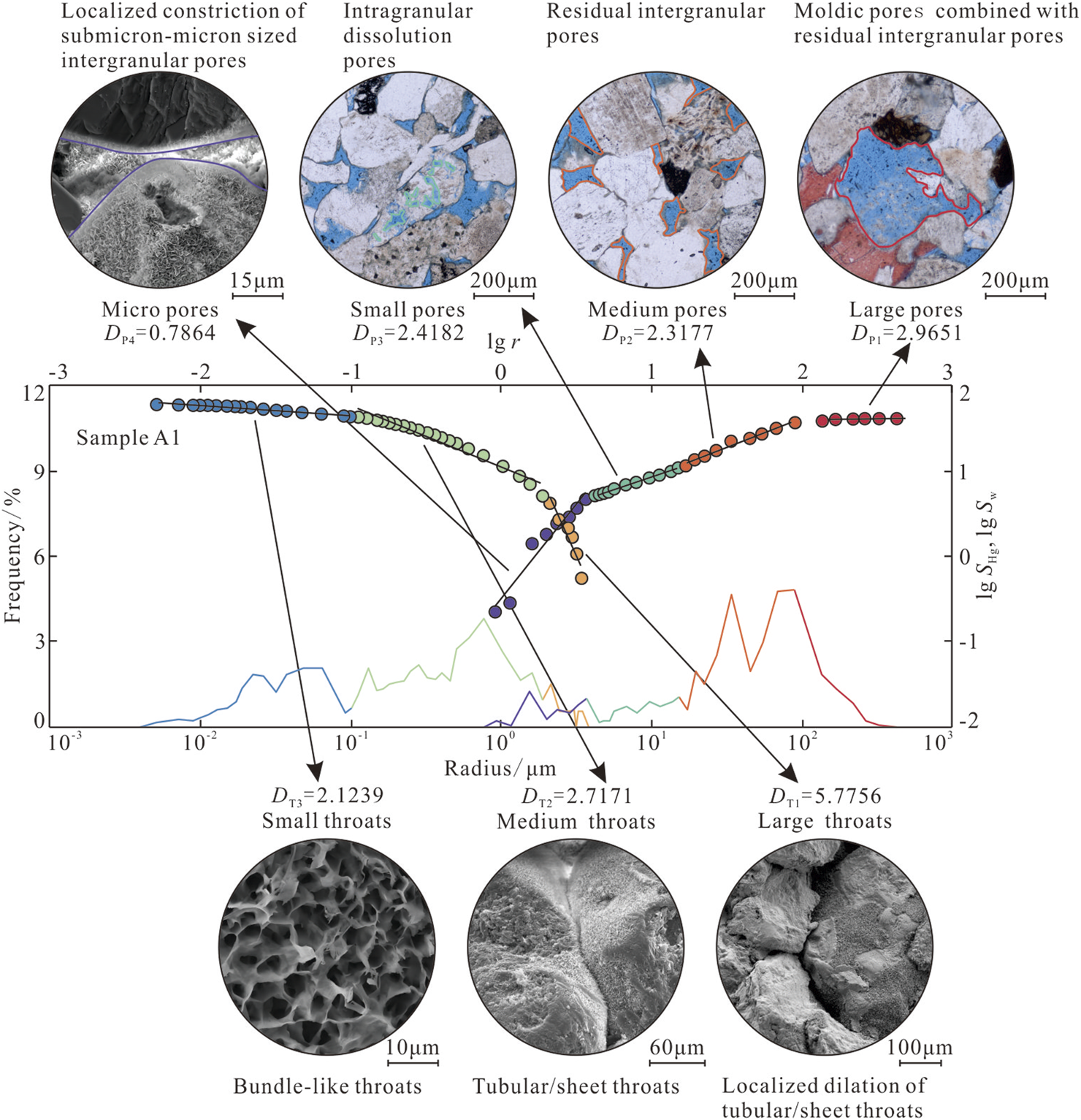
Microscopic characteristics and genetic types of the pore–throat system of sample A1.
In summary, integrating fractal characteristics and genetic origins, the pore–throat network of tight sandstone can be partitioned into seven distinct types: (1) small bundle-like throats developed within clay interstitial filler, (2) medium tubular/sheet throats generated by intense compaction, (3) large throats formed by local dilation of tubular throats, (4) micropores created by localized constriction of submicron-micron sized intergranular pores, (5) small pores dominated by intragranular dissolution pores, (6) medium pores comprised mainly of residual intergranular pores, and (7) large pores resulting from the combination of moldic pores and residual intergranular pores. Morphologically, these seven types interlink to establish a complex reservoir structure composed of throats that conform to the extension characteristics of the capillary tube model, and beaded pore–throat assemblages and pores that fit the extension characteristics of the spherical model, together defining a ternary structural framework.
Previous studies on the fractal characteristics of tight sandstones have proposed various pore–throat classification schemes. For example, based on the 3D capillary tube model, Zhu et al. (2019) analyzed HPMI data, identifying two distinct pore systems: capillary tube pores, which are relatively small and exhibit ideal fractal dimensions, and beaded pores, which are larger and display fractal dimensions exceeding 3. Similarly, Wang et al. (2023) applied the equivalent-sphere model to interpret NMR data, categorizing pores into shuttlecock pores, which are smaller in size with ideal fractal behavior, and the spiny-spherical pores, which are larger and exhibit fractal dimensions greater than 3. However, these schemes are limited by their reliance on a single technique with restricted scale coverage, which hinders comprehensive fractal characterization across the full-scale pore–throat distribution. Moreover, the applied methods do not clearly differentiate between pores and throats, and they overlook differences arising from their underlying geometric models. In contrast, the classification scheme proposed in this study is based on full-scale fractal analyses that separately evaluate pores and throats. It applies different models tailored to their morphological characteristics, thereby addressing key limitations of previous approaches. Coupled with an analysis of the genetic differences among pore–throat systems, this scheme revealed the origin of the divergence in pore–throat fractal dimensions and offers a more rational and holistic perspective for understanding reservoir heterogeneity in tight sandstones.
Although the sample set employed in this study is limited in number, it encompasses a wide range of physical properties and pore–throat parameters. Reservoirs of varying quality consistently exhibit ternary pore–throat structures and similar multi-scale fractal behavior. Therefore, the findings presented here have some general applicability and can be extrapolated to reservoirs with comparable lithology in other regions.
4.2 Analysis of factors influencing reservoir quality based on the pore–throat fractal systems classification
In this study, pore–throat systems were first classified by fractal dimension, and then evaluated in terms of how the porosity contribution of each system correlates with total porosity, permeability, and movable fluid saturation. Each system’s genetic origin was also considered to assess its impact on reservoir quality.
All pore systems show positive correlations with reservoir quality parameters, but the contributions of large pores and micropores are essentially uncorrelated (R2 = 0.0043–0.2548; Figures 14A–C, J–L). Medium pores exhibit the strongest correlation (R2 = 0.7829–0.8269; Figures 14D–F), followed by small pores (R2 = 0.4520–0.6399; Figures 14G–I).
FIGURE 14
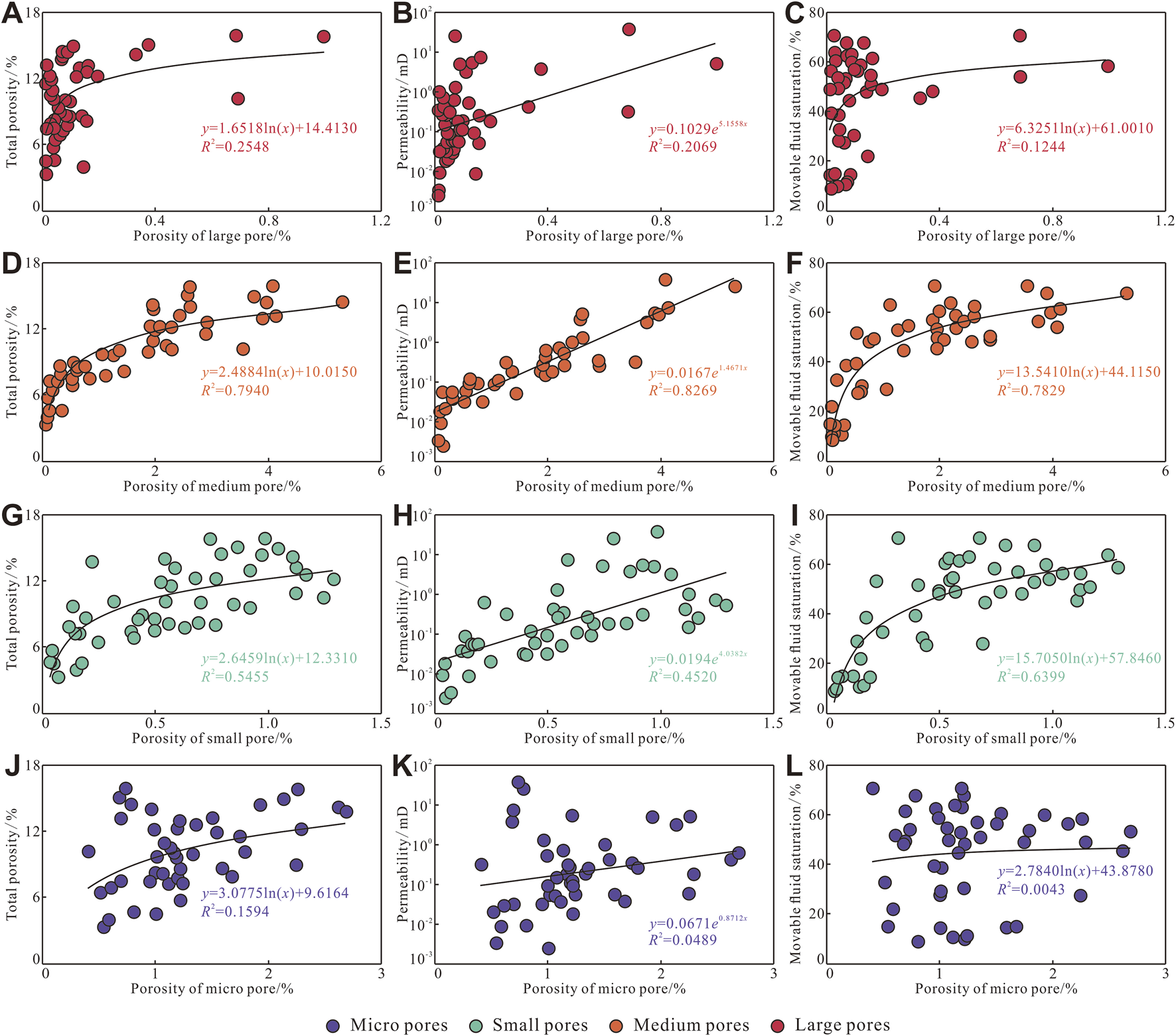
Effect of the pore system on reservoir quality. (A) Porosity of large pores vs. total porosity, (B) porosity of large pores vs. permeability, (C) porosity of large pores vs. movable fluid saturation, (D) porosity of the medium pores vs. total porosity, (E) porosity of medium pores vs. permeability, (F) porosity of medium pores vs. movable fluid saturation, (G) porosity of small pores vs. total porosity, (H) porosity of small pores vs. permeability, (I) Porosity of small pores vs. movable fluid saturation, (J) porosity of micropores vs. total porosity, (K) porosity of micropores vs. permeability, and (L) porosity of micropores vs. movable fluid saturation.
Throat systems likewise correlate positively with reservoir quality parameters, although large and small throats again display weak relationships (R2 = 0.0612–0.3402; Figures 15A–C, G–I). Medium throats correlate most strongly with total porosity and permeability (R2 = 0.7499 and 0.6584, respectively; Figures 15D,E), but less so with movable fluid saturation (R2 = 0.3939; Figure 15F).
FIGURE 15

Effect of the throat system on reservoir quality. (A) Porosity of large throats vs. total porosity, (B) porosity of large throats vs. permeability, (C) porosity of large throats vs. movable fluid saturation, (D) porosity of medium throats vs. total porosity, (E) porosity of medium throats vs. permeability, (F) porosity of medium throats vs. movable fluid saturation, (G) porosity of small throat vs. total porosity, (H) porosity of small throats vs. permeability, and (I) porosity of small throats vs. movable fluid saturation.
These results indicate that both total porosity and permeability are predominantly controlled by medium pores dominated by residual intergranular pores and medium throats composed of tubular/sheet throats. The abundance of these pores and throats is inversely proportional to compaction intensity. Thus, under relatively weak compaction, primary pores are better preserved and larger tubular throats develop more readily. Small pores, formed by intragranular dissolution, play a secondary role, with their development scaling with dissolution intensity. Medium pores also serve as the principal storage space for movable fluids, owing to their combination of a relatively large pore size and the highest porosity fraction.
For the target strata, relatively weak compaction emerges as the key factor in forming high-quality tight sandstone reservoirs, while dissolution processes provide an additional enhancement to reservoir performance. Future exploration should therefore emphasize reconstructing regional burial histories and clarifying the mechanisms of dissolution development.
5 Conclusion
This study integrates HPMI, CRMI, and NMR to characterize full-scale pore and throat distributions in tight sandstones, computes fractal dimensions using appropriate models, classifies pore–throat systems by fractal characters, identifies their genetic types, and evaluates each type’s impact on reservoir quality. The main conclusions are
Fractal behavior varies across scales. Seven genetic pore–throat systems are recognized: small bundle-like throats developed within clay interstitial filler, medium tubular/sheet throats generated by intense compaction, large throats formed by local dilation of tubular/sheet throats, micropores created by localized constriction of submicron-micron sized intergranular pores, small pores dominated by intergranular dissolution pores, medium pores comprised mainly of residual intergranular pores, and large pores resulting from the combination of moldic pores and residual intergranular pores.
- 2.
Small and medium throats conform to the capillary tube assumption, with DT1 = 2.1168–2.3923 (mean 2.2093) and DT2 = 2.4098–2.9393 (mean 2.7214). Small, medium, and large pores follow the spherical pore assumption, yielding DP2 = 2.4182–2.9902 (mean 2.8180), DP3 = 2.3177–2.9661 (mean 2.7435), and DP4 = 2.8701–2.9988 (mean 2.9825), respectively. Large throats and micropores overlap in size and form beaded features; under standard models, their computed fractal dimensions fall outside the ideal 2–3 range. Consequently, tight sandstone storage is best conceptualized as a ternary network of capillary-like throats, bead-like pore throats, and spherical pores.
- 3.
Correlation analysis shows that total porosity and permeability are governed primarily by medium pores and medium throats, with small pores as a secondary influence. Medium pores also provide the main space for movable fluids. Relatively weak compaction emerges as the key factor for high-quality reservoir development in the strata studied, while dissolution further enhances reservoir quality to a lesser degree.
Statements
Data availability statement
The raw data supporting the conclusions of this article will be made available by the authors, without undue reservation.
Author contributions
LF: Conceptualization, Methodology, Writing – original draft, Formal analysis, Investigation. RW: Data curation, Project administration, Resources, Writing – review and editing. NL: Software, Validation, Writing – review and editing. ZG: Supervision, Visualization, Writing – review and editing.
Funding
The authors declare that no financial support was received for the research and/or publication of this article.
Conflict of interest
Authors LF, RW, NL, and ZG were employed by the Natural Gas Research Institute of Yanchang Petroleum (Group) Co., Ltd.
Generative AI statement
The authors declare that no Generative AI was used in the creation of this manuscript.
Any alternative text (alt text) provided alongside figures in this article has been generated by Frontiers with the support of artificial intelligence and reasonable efforts have been made to ensure accuracy, including review by the authors wherever possible. If you identify any issues, please contact us.
Publisher’s note
All claims expressed in this article are solely those of the authors and do not necessarily represent those of their affiliated organizations, or those of the publisher, the editors and the reviewers. Any product that may be evaluated in this article, or claim that may be made by its manufacturer, is not guaranteed or endorsed by the publisher.
References
1
Cheng Y. Luo X. Hou B. Zhang S. Tan C. Xiao H. (2023). Pore structure and permeability characterization of tight sandstone reservoirs: from a multiscale perspective. Energy. Fuels.37 (13), 9185–9196. 10.1021/acs.energyfuels.3c01693
2
Coates G. Xiao L. Primmer M. G. (1999). NMR logging principles and applications. Houston, USA: Gulf Publishing, 57–65.
3
Daigle H. Johnson A. (2016). Combining Mercury intrusion and nuclear magnetic resonance measurements using percolation theory. Transport. Porous. Med111, 669–679. 10.1007/s11242-015-0619-1
4
Dou W. Liu L. Jia L. Xu Z. Wang M. Du C. (2021). Pore structure, fractal characteristics and permeability prediction of tight sandstones: a case study from Yanchang Formation, Ordos Basin, China. Mar. Petrol. Geol.123, 104737. 10.1016/j.marpetgeo.2020.104737
5
Guo X. Huang Z. Zhao L. Han W. Ding C. Sun X. et al (2019). Pore structure and multi-fractal analysis of tight sandstone using MIP, NMR and NMRC methods: a case study from the Kuqa depression, China. J. Petrol. Sci. Eng.178, 544–558. 10.1016/j.petrol.2019.03.069
6
Guo R. Xie Q. Qu X. Chu M. Li S. Ma D. et al (2020). Fractal characteristics of pore-throat structure and permeability estimation of tight sandstone reservoirs: a case study of Chang 7 of the Upper Triassic Yanchang Formation in Longdong area, Ordos Basin, China. J. Petrol. Sci. Eng.184, 106555. 10.1016/j.petrol.2019.106555
7
Han Y. Jiang Z. Liang Z. Lai Z. Liang H. Wu Y. et al (2023). Full pore size fractal characteristics of Longmaxi formation shale in Luzhou-Changning area and its influence on seepage. Energy. Fuels.37 (15), 11083–11096. 10.1021/acs.energyfuels.3c01456
8
He T. Zhou Y. Chen Z. Zhang Z. Xie H. Shang Y. et al (2024). Fractal characterization of the pore-throat structure in tight sandstone based on low-temperature nitrogen gas adsorption and high-pressure mercury injection. Fractal. Fract.8, 356. 10.3390/fractalfract8060356
9
Huang W. Lu S. Hersi O. S. Wang M. Deng S. Lu R. (2017). Reservoir spaces in tight sandstones: classification, fractal characters, and heterogeneity. J. Petrol. Sci. Eng.46, 80–92. 10.1016/j.jngse.2017.07.006
10
Katz A. Thompson A. (1985). Fractal sandstone pores: implications for conductivity and pore formation. Phys. Rev. Lett.54, 1325–1328. 10.1103/PhysRevLett.54.1325
11
Kleinberg R. Horsfield M. (1990). Transverse relaxation processes in porous sedimentary rock. J. Magn. Reson.88, 9–19. 10.1016/0022-2364(90)90104-H
12
Krohn C. (1988). Fractal measurements of sandstones, shales, and carbonates. J. Geophys. Res.93, 3297–3305. 10.1029/JB093iB04p03297
13
Li K. (2010). Analytical derivation of Brooks-Corey type capillary pressure models using fractal geometry and evaluation of rock heterogeneity. J. Petrol. Sci. Eng.73, 20–26. 10.1016/j.petrol.2010.05.002
14
Li K. Horne R. (2006). Fractal modeling of capillary pressure curves for the Geysers rocks. Geothermics35, 198–207. 10.1016/j.geothermics.2006.02.001
15
Liu L. Liu X. Sang Q. Li W. Xiong J. Liang L. (2024). Pore‐throat structure and fractal characteristics of tight gas sandstone reservoirs: a case study of the second member of the Upper Triassic Xujiahe Formation in zhongba area, western Sichuan depression, China. Geol. J.59, 1879–1891. 10.1002/gj.4975
16
Liu S. Wang M. Cheng Y. Yu X. Duan X. Kang Z. et al (2025). Fractal insights into permeability control by pore structure in tight sandstone reservoirs, Heshui area, Ordos Basin. Geosciences17 (1), 20250791. 10.1515/geo-2025-0791
17
Mandelbrot B. Passoja D. Paullay D. (1984). Fractal character of fracture surfaces in porous media. Nature308, 721–722. 10.1038/308721a0
18
Meng M. Ge H. Ji W. Wang X. (2016). Research on the auto-removal mechanism of shale aqueous phase trapping using low field nuclear magnetic resonance technique. J. Petrol. Sci. Eng.137, 63–73. 10.1016/j.petrol.2015.11.012
19
Nan F. Lin L. Lai Y. Wang C. Yu Y. Chen Z. (2023). Research on fractal characteristics and influencing factors of pore-throats in tight sandstone reservoirs: a case Study of Chang 6 of the Upper Triassic Yanchang Formation in huaqing area, ordos Basin, China. Minerals. 13(9): 1137. 10.3390/min13091137
20
Pan Y. Huang Z. Li T. Xu X. Chen X. Guo X. (2021). Pore structure characteristics and evaluation of lacustrine mixed fine-grained sedimentary rocks: a case study of the Lucaogou Formation in the Malang Sag, Santanghu Basin, Western China. J. Petrol. Sci. Eng.201, 108545. 10.1016/j.petrol.2021.108545
21
Qiao J. Zeng J. Jiang S. Zhang Y. Feng S. Feng X. et al (2020). Insights into the pore structure and implications for fluid flow capacity of tight gas sandstone: a case study in the upper paleozoic of the Ordos basin. Mar. Petrol. Geol.118, 104439. 10.1016/j.marpetgeo.2020.104439
22
Qiao J. Zeng J. Chen D. Cai J. Jiang S. Xiao E. et al (2022). Permeability estimation of tight sandstone from pore structure characterization. Mar. Petrol. Geol.135, 105382. 10.1016/j.marpetgeo.2021.105382
23
Qu Y. Sun W. Tao R. Luo B. Chen L. Ren D. (2020). Pore–throat structure and fractal characteristics of tight sandstones in yanchang Formation, Ordos Basin. Mar. Petrol. Geol.120, 104573. 10.1016/j.marpetgeo.2020.104573
24
Wang F F. Jiao L. Liu Z. Tan X. Wang C. Gao J. (2018). Fractal analysis of pore structures in low permeability sandstones using Mercury intrusion porosimetry. J. POROUS. MEDIA.21 (11), 1097–1119. 10.1615/JPorMedia.2018021393
25
Wang X X. Hou J. Song S. Wang D. Gong L. Ma K. et al (2018). Combining pressure-controlled porosimetry and rate-controlled porosimetry to investigate the fractal characteristics of full-range pores in tight oil reservoirs. J. Petrol. Sci. Eng.71, 353–361. 10.1016/j.petrol.2018.07.050
26
Wang W. Wang R. Wang L. Qu Z. Ding X. Gao C. et al (2023). Pore structure and fractal characteristics of tight sandstones based on nuclear magnetic resonance: a case Study in the Triassic Yanchang Formation of the ordos Basin, China. ACS Omega8, 16284–16297. 10.1021/acsomega.3c00937
27
Wang J. Zhang J. Xiao X. Chen Y. H D. (2024a). Pore structure and fractal characteristics of inter-layer sandstone in marine-continental transitional shale: a case Study of the Upper Permian longtan Formation in Southern Sichuan Basin, south China. Fractal. Fract.9, 11. 10.3390/fractalfract9010011
28
Wang W. Lin C. Zhang X. (2024b). Fractal dimension analysis of pore throat structure in tight sandstone reservoirs of Huagang Formation: jiaxing area of East China Sea Basin. Fractal. Fract.8, 374. 10.3390/fractalfract8070374
29
Wang W. Lin C. Zhang X. (2024c). Fractal characteristics of pore throat and throat of tight sandstone sweet spot: a case Study in the East China Sea Basin. Fractal. Fract.8, 684. 10.3390/fractalfract8120684
30
Wang F F. Zeng F. Wang L. Hou X. Cheng H. Gao J. (2021). Fractal analysis of tight sandstone petrophysical properties in unconventional oil reservoirs with NMR and rate-controlled porosimetry. Energy. Fuels.35, 3753–3765. 10.1021/acs.energyfuels.0c03394
31
Wang J J. Jiang F. Zhang C. Song Z. Mo W. (2021). Study on the pore structure and fractal dimension of tight sandstone in coal measures. Energy. Fuels.35, 3887–3898. 10.1021/acs.energyfuels.0c03991
32
Wang W W. Yue D. Eriksson K. Qu X. Li W. Lv M. et al (2020). Quantification and prediction of pore structures in tight oil reservoirs based on multifractal dimensions from integrated pressure-and rate-controlled porosimetry for the upper Triassic Yanchang formation, Ordos Basin, China. Energy. Fuels.34, 4366–4383. 10.1021/acs.energyfuels.0c00178
33
Wang Z Z. Jiang X. Pan M. Shi Y. (2020). Nano-scale pore structure and its multi-fractal characteristics of tight sandstone by n2 adsorption/desorption analyses: a case study of shihezi formation from the sulige gas filed, ordos basin, China. Minerals10, 377. 10.3390/min10040377
34
Washburn E. (1921). The dynamics of capillary flow. Phys. Rev.17, 273–283. 10.1103/PhysRev.17.273
35
Wu Y. Tahmasebi P. Lin C. Zahid M. Dong C. Golab A. et al (2019). A comprehensive study on geometric, topological and fractal characterizations of pore systems in low-permeability reservoirs based on SEM, MICP, NMR, and X-ray CT experiments. Mar. Petrol. Geol.103, 12–28. 10.1016/j.marpetgeo.2019.02.003
36
Wu F F. Li Y. Burnham B. Zhang Z. Yao C. Yuan L. et al (2022). Fractal-based NMR permeability estimation in tight sandstone: a case study of the Jurassic rocks in the Sichuan Basin, China. J. Petrol. Sci. Eng.218, 110940. 10.1016/j.petrol.2022.110940
37
Wu Y Y. Liu C. Ouyang S. Luo B. Zhao D. Sun W. et al (2022). Investigation of pore-throat structure and fractal characteristics of tight sandstones using HPMI, CRMI, and NMR methods: a case study of the lower Shihezi formation in the sulige area, Ordos Basin. J. Petrol. Sci. Eng.210, 110053. 10.1016/j.petrol.2021.110053
38
Xiao D. Lu S. Lu Z. Huang W. Gu M. (2016). Combining nuclear magnetic resonance and rate-controlled porosimetry to probe the pore-throat structure of tight sandstones. Petrol. Explor. Dev.43, 961–970. 10.11698/PED.2016.06.13
39
Xie W. Yin Q. Zeng J. Wang G. Feng C. Zhang P. (2023). Fractal-based approaches to pore structure investigation and water saturation prediction from NMR measurements: a case study of the gas-bearing tight sandstone reservoir in Nanpu Sag. Fractal. Fract.7, 273. 10.3390/fractalfract7030273
40
Xin Y. Wang G. Liu B. Ai Y. Cai D. Yang S. et al (2022). Pore structure evaluation in ultra-deep tight sandstones using NMR measurements and fractal analysis. J. Petrol. Sci. Eng.211, 110180. 10.1016/j.petrol.2022.110180
41
Xu S. Yang Z. Wu S. Wang L. Wei W. Yang F. et al (2022). Fractal analysis of pore structure differences between shale and sandstone based on the nitrogen adsorption method. Nat. Resour. Res.31, 1759–1773. 10.1007/s11053-022-10056-5
42
Yang Y. Xiao W. Zheng L. Lei Q. Qin C. He Y. et al (2023). Pore throat structure heterogeneity and its effect on gas-phase seepage capacity in tight sandstone reservoirs: a case study from the Triassic Yanchang Formation, Ordos Basin. Petrol. Sci.20, 2892–2907. 10.1016/j.petsci.2023.03.020
43
Yang M. Pan Y. Feng H. Yan Q. Lu Y. Wang W. et al (2024a). Fractal characteristics of pore structure of longmaxi shales with different burial depths in Southern Sichuan and its geological significance. Fractal. Fract.9 (1), 2. 10.3390/fractalfract9010002
44
Yang Y. Wen Z. Tian W. Fan Y. Gao H. (2024b). A new model for predicting permeability of Chang 7 tight sandstone based on fractal characteristics from high-pressure Mercury injection. Energies17, 821. 10.3390/en17040821
45
Yao Y. Liu D. (2012). Comparison of low-field NMR and mercury intrusion porosimetry in characterizing pore size distribution of coals. Fuel95, 152–158. 10.1016/j.fuel.2011.12.039
46
Zang Q. Liu C. Awan R. Yang X. Li G. Wu Y. et al (2022). Occurrence characteristics of the movable fluid in heterogeneous sandstone reservoir based on fractal analysis of NMR data: a case study of the Chang 7 Member of Ansai Block, Ordos Basin, China. J. Petrol. Sci. Eng.214, 110499. 10.1016/j.petrol.2022.110499
47
Zhang X. Wu C. Li T. (2017). Comparison analysis of fractal characteristics for tight sandstones using different calculation methods. J. Geopghys. Eng.14, 120–131. 10.1088/1742-2140/14/1/120
48
Zhang F. Jiang Z. Sun W. Li Y. Zhang X. Zhu L. et al (2019). A multiscale comprehensive study on pore structure of tight sandstone reservoir realized by nuclear magnetic resonance, high pressure mercury injection and constant-rate mercury injection penetration test. Mar. Petrol. Geol.109, 208–222. 10.1016/j.marpetgeo.2019.06.019
49
Zhang K. Lai J. Bai G. Pang X. Ma X. Qin Z. et al (2020). Comparison of fractal models using NMR and CT analysis in low permeability sandstones. Mar. Petrol. Geol.112, 104069. 10.1016/j.marpetgeo.2019.104069
50
Zhang B. Wang H. Sun B. Ouyang Z. Dou W. Wang B. et al (2024). Pore size distribution and fractal characteristics of deep coal in the Daning–Jixian block on the Eastern Margin of the ordos Basin. Acs. Omega.9(30): 32837–32852. 10.1021/acsomega.4c03510
51
Zhao D. Hou J. Sarma H. Guo W. Liu Y. Xie P. et al (2023). Zhang, Z.Y. Pore throat heterogeneity of different lithofacies and diagenetic effects in gravelly braided river deposits: implications for understanding the formation process of high-quality reservoirs. Geoenegry. Sci. Eng.221, 111309. 10.1016/j.petrol.2022.111309
52
Zhu H. Zhang T. Zhong D. Li Y. Zhang J. Chen X. (2019). Binary pore structure characteristics of tight sandstone reservoirs. Petrol. Explor. Dev.46, 1220–1228. 10.11698/PED.2019.06.20
53
Zhu H. Ju Y. Lu Y. Yang M. Feng H. Qiao P. et al (2025). Natural evidence of organic nanostructure transformation of shale during bedding-parallel slip. Geol. Soc. Am. Bull.137(5-6): 2719–2746. 10.1130/B37712.1
Summary
Keywords
controlling factor, ternary pore–throat structure, pore–throat system, fractal dimension, full-scale, reservoir, tight sandstone
Citation
Feng L, Wang R, Liu N and Gao Z (2026) Fractal characteristics of full-scale pores and throats in tight sandstone and their application in the analysis of the main controlling factors of a reservoir. Front. Earth Sci. 13:1701181. doi: 10.3389/feart.2025.1701181
Received
08 September 2025
Revised
11 November 2025
Accepted
26 November 2025
Published
06 January 2026
Volume
13 - 2025
Edited by
Li Ang, Jilin University, China
Reviewed by
Hongjian Zhu, Yanshan University, China
Jinsui Wu, Khalifa University, United Arab Emirates
Updates
Copyright
© 2026 Feng, Wang, Liu and Gao.
This is an open-access article distributed under the terms of the Creative Commons Attribution License (CC BY). The use, distribution or reproduction in other forums is permitted, provided the original author(s) and the copyright owner(s) are credited and that the original publication in this journal is cited, in accordance with accepted academic practice. No use, distribution or reproduction is permitted which does not comply with these terms.
*Correspondence: Linjie Feng, geofeng1993@163.com
Disclaimer
All claims expressed in this article are solely those of the authors and do not necessarily represent those of their affiliated organizations, or those of the publisher, the editors and the reviewers. Any product that may be evaluated in this article or claim that may be made by its manufacturer is not guaranteed or endorsed by the publisher.