Analysis and testing of the detection performance of an ultra-deep azimuthal electromagnetic logging-while-drilling tool

With the increasing complexity of hydrocarbon reservoirs, there is growing demand for greater depth of detection (DoD) in electromagnetic (EM) logging-while-drilling (LWD) tools. The latest generation of ultra-deep azimuthal resistivity LWD systems can reach several tens of meters, enabling precise geosteering, reservoir-scale geological understanding, and optimized field development. This study introduces a newly developed ultra-deep azimuthal EM LWD instrument. Sensitivity analysis of multi-component induced electromotive force (EMF) was performed with respect to resistivity and formation boundaries, identifying the most effective components for boundary detection. Measurement modes were then constructed to separate resistivity and boundary-sensitive signals. Transmitter–receiver spacing and operating frequency were optimized by jointly considering signal dynamics and gain, yielding an optimal range of 5–7 m spacing and 10–50 kHz frequency. A quantitative method was established to characterize maximum boundary-detection capability by integrating signal dynamic range (DR) and system measurement error. Under 80 dB DR and ±5% error, the tool achieved a DoD of 36.4 m. To validate performance, an airhang test model was developed, and finite element simulations were conducted to define test conditions by accounting for shoreline and crane interference. Airhang verification tests are conducted with the instrument parallel to the sea surface. And the measurement results show good agreement with the numerical simulation results. The instrument’s actual DoD exceeds 30 m, representing a significant improvement compared to conventional LWD azimuthal resistivity tool, confirming its value for deep boundary detection in complex geological environments.

1 Introduction

With global hydrocarbon exploration extending into increasingly complex geological structures, deep water environments, and unconventional reservoirs, conventional logging technologies face critical challenges such as limited depth of investigation, insufficient resolution, and inadequate real-time capability (Bergeron et al., 2022). Electromagnetic (EM) logging-while-drilling (LWD) has become a core technology for geosteering and reservoir evaluation. Its performance directly impacts drilling efficiency, reservoir contact, and overall exploration and production costs.

The operating principle of EM LWD is based on EM induction. An alternating current is applied to the transmitter, generating a primary EM field in the formation. This induces eddy currents, which in turn act as secondary field sources, producing secondary EM fields. By accurately measuring the amplitude and phase of the secondary fields, the formation conductivity can be inverted in real time (Rodney et al., 1983). Since its commercialization in the 1990s, EM LWD technology has undergone three distinct stages of development: conventional resistivity LWD, azimuthal resistivity LWD, and ultra-deep azimuthal resistivity LWD, with each stage driven by specific technical breakthroughs and engineering demands.

Stage I (1990s–2000s): Conventional resistivity LWD. Building upon wireline logging principles, the first generation of EM LWD tools (e.g., ARC, MPR, EWR) were introduced by companies such as Schlumberger and Baker Hughes. These tools employed basic coaxial coil configurations with dual receivers, measuring amplitude ratio and phase shift of the magnetic field’s zz-component to estimate formation resistivity. With a typical investigation depth of only 1–2 m, these tools were primarily applied for geosteering in conventional sandstone reservoirs drilled with high-angle wells (Bittar et al., 1991).

Stage II (2005–2015): Azimuthal resistivity LWD. With the proliferation of horizontal wells, the industry advanced EM LWD technology by introducing cross-component (e.g., xz and zx) measurements to enhance azimuthal sensitivity and improve boundary detection. Second-generation azimuthal resistivity tools (e.g., PeriScope, AziTrak, ADR, BWPR, AMR) employed three common configurations: (1) axial transmitters/receivers combined with orthogonal receivers/transmitters; (2) axial transmitters combined with tilted receivers; (3) tilted transmitters combined with tilted receivers. With DoD of 5–7 m and supported by 1D boundary inversion, these tools enabled accurate estimation of resistivity and boundary distance, driving the leapfrog development of EM LWD from “reactive geosteering” to “proactive geosteering” (Omeragic et al., 2005; Bell et al., 2006; Bittar et al., 2009; Yang et al., 2013; Yang et al., 2016; Yue et al., 2022; Wang et al., 2023a; Wang et al., 2025; Wang et al., 2023b).

Stage III (2016–present): Ultra-deep azimuthal resistivity LWD. As reservoir development has expanded into unconventional resources and complex geological structures, the limitations of conventional azimuthal tools have become apparent. Ultra-deep azimuthal resistivity technologies (e.g., GeoSphere, VisiTrak, EarthStar) have since emerged (Seydoux et al., 2014; Hartmann et al., 2014; Wu et al., 2018). Their key features include: operating at lower frequencies (2–100 kHz) and longer transmitter–receiver spacings (>10 m), achieving detection depths exceeding 60 m; employing full-tensor field measurements for enhanced anisotropy characterization; and incorporating advanced inversion schemes powered by cloud-based platforms. In addition, there are also ultra-deep look-ahead LWD services, such as IriSphere and BrightStar, which enable real-time detecting of geological structures ahead of the drill bit when the reservoir could not be mapped from seismic measurements. These tools can achieve a maximum look-ahead distance exceeding 30 m, providing critical guidance for geostopping and drilling decisions. Ultra-deep resistivity marks a paradigm shift for EM LWD—from well placement guidance to reservoir-scale imaging (Huang and Yang, 2020; Wu et al., 2022; Yuan et al., 2022; Singh et al., 2021; Ma et al., 2022; Salim et al., 2025; Holmquist et al., 2025; Wu et al., 2024).

The development of ultra-deep azimuthal resistivity tools requires overcoming several challenges, including: reliable transmission and reception of low-frequency signals over a wide dynamic range (DR), antenna system design, suppression of inversion non-uniqueness, and efficient telemetry of large volumes of data. We have newly developed the ultra-deep azimuthal resistivity tool (UD-AMR) building upon the foundation of the azimuthal resistivity tool (AMR). This paper presents the design, optimization, and testing of UD-AMR. Specifically, we analyze the sensitivity of induced electromotive force (EMF) components to geological parameters to identify the most effective; establish operating modes for ultra-deep resistivity and boundary detection; optimize spacing and operating frequency, design antenna configurations accordingly, and validate tool performance through airhang experiments. This study provides technical insights to guide the further development of next-generation ultra-deep azimuthal EM LWD systems.

2 Sensitivity analysis and optimization of induced EMF components

To identify the most suitable induced EMF components for ultra-deep resistivity and boundary detection, we first analyzed, from a macroscopic perspective, the sensitivity of both the real and imaginary parts of all EMF components to different geological parameters. Equation 1 presents the definition of the sensitivity function.

$S_{ij}=\frac{\mathrm{\partial }{V}_{ij}}{\mathrm{\partial }x},x=\alpha ,\beta ,p\cdots (1)$

where $V_{ij}$ denotes the induced EMF component, α is the dip angle; β is the azimuth, i.e., the toolface angle; both α and β are measured in degrees; and p represents the boundary position. For a two-layer formation model, the sensitivity of each EMF component is evaluated using a finite-difference perturbation approach. Specifically, the difference between the tool responses after a small perturbation of a geological parameter (Δ) and the baseline responses is computed and normalized by the magnitude of the perturbation. In our study, Δ is set to 0.01. The sensitivity of $V_{ij}$ to inclination, azimuth and boundary position are the derivatives of EMF response with respect to inclination (Volt/degree), azimuth (Volt/degree), and boundary position (Volt/m).

A two-layer formation model was constructed with resistivities of 10 Ω m and 1 Ω m respectively. A triaxial transmitter–receiver configuration is used with a spacing of 6 m and an operating frequency of 20 kHz. The tool is positioned near the formation boundary. Figure 1 illustrates the simulated sensitivities of the real and imaginary parts of EMF components to formation azimuth.

Figure 1

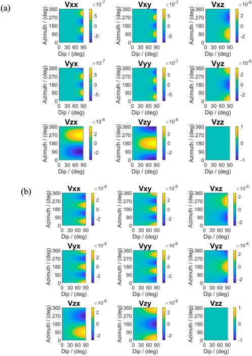
Figure 1. Sensitivity of EMF components with respect to azimuth (R1 = 10 Ω m, R2 = 1 Ω m). (a) Imaginary part; (b) real part.

Results show that the xx, xy, yx, and yy components have sensitivities with a periodicity of π, meaning their responses are symmetric when the boundary is located above or below the tool, and thus they cannot distinguish boundary position relative to the tool. By contrast, the xz, yz, zx, and zy components exhibit sensitivities with a 2π periodicity, where responses are opposite in sign for boundaries located above versus below the tool, making them suitable for boundary detection. The zz component shows no azimuthal sensitivity. Furthermore, comparisons among xz, yz, zx, and zy components indicate opposite sensitivities between paired components (e.g., xz vs. zx, yz vs. zy), enabling complex signal synthesis.

Figure 2 further shows the sensitivities of EMF components to boundary position. For small inclination, the xz, yz, zx, and zy components are relatively insensitive to boundary, particularly in vertical wells. With increasing inclination, sensitivity improves significantly, explaining why boundary detection is more effective in high-angle and horizontal wells. The sensitivities are strongest at toolfaces of 0°/360° and 180°, while diminishing at other orientations. The zz component becomes more sensitive to boundaries in horizontal wells due to the so-called horn effect.

Figure 2

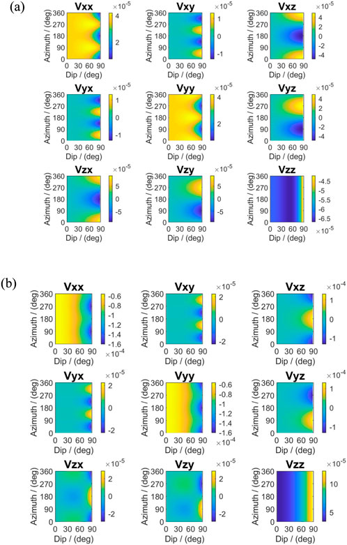
Figure 2. Sensitivity of EMF components with respect to boundary position (R1 = 10 Ω m, R2 = 1 Ω m). (a) Imaginary part; (b) real part.

To clarify which components and which parts (real or imaginary) are best suited for boundary detection, Figure 3 compares the responses of the xz and zx components in both real and imaginary parts for a two-layer model, where the formation resistivities are 100 and 1 Ω m, respectively. The spacing is 6 m and the frequency is 20 kHz. Results show that the imaginary parts extend farther than the real parts in terms of detectable range. Therefore, the imaginary part of the xz/zx components, or a combination of their amplitudes with the sign of the imaginary part, can be defined as the boundary detection signal.

Figure 3

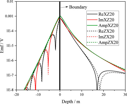
Figure 3. Comparison of real and imaginary parts of xz and zx induced EMF components.

3 Measurement modes of ultra-deep azimuthal resistivity

To achieve both near-wellbore and deep formation detection, an antenna configuration is designed for UD-AMR, as shown in Figure 4. The tool consists of two parts: a tilted-transmitter sub and the main instrument body. In the main body, the Tc transmitter and the R2 receiver are configured for deep boundary detection. Tc is composed of a pair of orthogonal multi-turn transverse coils (Tcx and Tcy), ensuring that even during sliding drilling, EMF signals from two bins can be simultaneously measured for boundary detection. R2 is a multi-turn axial coil.

Figure 4

Figure 4. Antenna configuration of the UD-AMR tool.

The independent tilted-transmitter sub (T1) enables resistivity measurement by combining the responses of receivers R1 and R2. By analyzing attention and phase shift, resistivity can be derived. In this configuration, T1 is a multi-turn tilted coil, while R1 is a multi-turn axial coil. The transmitter spacing and operating frequency are adjustable depending on formation characteristics. Additionally, the instrument body integrates a AMR for near-wellbore detection, the details of which are documented elsewhere.

The ultra-deep resistivity mode employs a tilted-transmitter with dual axial receivers. Owing to the tilted transmitter, both zz and xz components can be measured simultaneously, which reflect azimuthal resistivity. Equation 2 defines the attenuation and phase shift between R1 and R2. Figure 5 shows the resistivity conversion charts for attenuation and phase shift. For spacing of [12 17] m and frequencies of 20 kHz and 50 kHz, the phase-shift resistivity has a much broader measurement range than attenuation resistivity. These conversion charts can be used to transform measured signals into equivalent resistivities.

$\begin{array}{l}Att=20\lg \frac{\sqrt{{\left(\text{Re}\left[V_1\right]\right)}^2+{\left(\text{Im}\left[V_1\right]\right)}^2}}{\sqrt{{\left(\text{Re}\left[V_2\right]\right)}^2+{\left(\text{Im}\left[V_2\right]\right)}^2}}\\ PS={\tan }^{-1}\frac{\text{Im}\left[V_2\right]}{\text{Re}\left[V_2\right]}-{\tan }^{-1}\frac{\text{Im}\left[V_1\right]}{\text{Re}\left[V_1\right]}\end{array}(2)$

where V₁ and V₂ denotes the induced EMF component of R1 and R2 respectively.

Figure 5

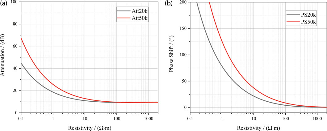
Figure 5. Conversion charts of resistivity from (a) attenuation and (b) phase shift.

The accuracy of attenuation and phase-shift acquisition circuits directly determines resistivity measurement range and accuracy. For a given target resistivity range and accuracy requirement, the acquisition precision of both parameters must meet corresponding specifications. Figure 6 illustrates the effects of acquisition accuracy on resistivity inversion. At low resistivity, large base values minimize the influence of measurement errors. At high resistivity, however, both parameters approach small values, causing significant error in resistivity. For instance, when phase-shift detection precision reaches ±0.3°, the tool can achieve a resistivity measurement range of 0.1–2000 Ω m, with accuracy equivalent to 0.3 ms/m.

Figure 6

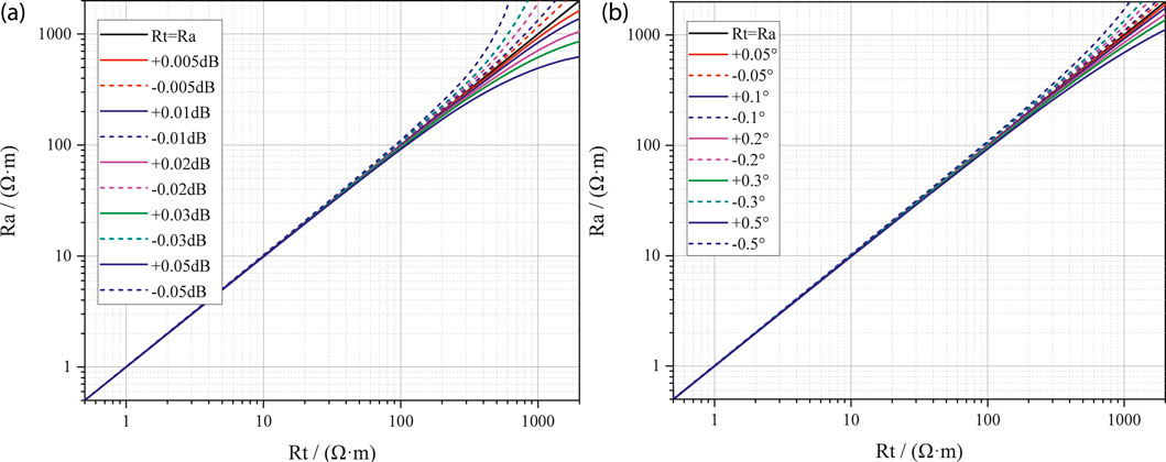
Figure 6. Effect of attenuation and phase-shift acquisition accuracy on resistivity measurement. (a) attenuation; (b) phase-shift.

For boundary detection, the UD-AMR system utilizes the xz component of EMF measured with Tc transmitter and R2 receiver, along with geosignals from T1 transmitter and R1/R2 receiver. Equation 3 can be used to calculate the xz EMF.

$V_{xz}=-i\omega N_T{N}_{R}s\mu H_{xz}(3)$

where i is the imaginary unit, N_T and N_R are the number of transmitter and receiver coils respectively, s is the coil area, μ is the magnetic permeability, M is the magnetic moment, and H_xz is the xz component of magnetic field and Equation 4 presents the definition of the geosignals.

$\begin{array}{l}{G}_{Att}=20\lg \frac{\sqrt{{\left(\text{Re}\left[V_{\beta }\right]\right)}^2+{\left(\text{Im}\left[V_{\beta }\right]\right)}^2}}{\sqrt{{\left(\text{Re}\left[V_{\left(\beta +\pi \right)}\right]\right)}^2+{\left(\text{Im}\left[V_{\left(\beta +\pi \right)}\right]\right)}^2}}\\ G_{PS}={\tan }^{-1}\frac{\text{Im}\left[V_{\beta }\right]}{\text{Re}\left[V_{\beta }\right]}-{\tan }^{-1}\frac{\text{Im}\left[V_{\left(\beta +\pi \right)}\right]}{\text{Re}\left[V_{\left(\beta +\pi \right)}\right]}\end{array}(4)$

where G_Att and G_PS denote the attenuation and phase-shift geosignals for boundary detection, respectively. V_β and V_β+π represent the measured EMF at toolface angles β and β + π. Typically, β is set to zero.

A three-layer formation model is constructed with resistivities of 1, 10 and 1 Ω m, respectively. The tool penetrates the target layer upward at a well inclination of 85°, and Figure 7 shows the corresponding tool responses for both AMR and UD-AMR. The AMR-derived resistivity curves accurately reflect the true formation resistivity. In contrast, UD-AMR responses show resistivity variation even when relatively far from the target, indicating its sensitivity to distant boundaries but also necessitating inversion for quantitative resistivity extraction.

Figure 7

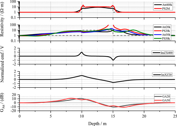
Figure 7. Measurements by UD-AMR.

Furthermore, due to the tilted transmitter, UD-AMR responses exhibit azimuthal asymmetry, with significant differences near both formation interfaces. When normalized, UD-AMR boundary-detection signals reveal earlier indications of boundary compared to AMR, while geological signals from T1 provide additional confirmation, enriching the measurement information.

It should be noted that EM LWD inversion typically concatenates resistivity and boundary-detection data into a single vector for optimization. However, mixing data of different attributes and magnitudes can distort inversion outcomes. The two types of boundary-detection signals defined here provide complementary azimuthal sensitivity with different DoD, but should be paired individually with resistivity data in inversion schemes rather than combined. The availability of multi-spacing, multi-frequency data from UD-AMR supports this differentiated processing.

4 Optimization of spacing and frequency

For ultra-deep azimuthal resistivity LWD tools, the boundary-detection signal measured by Tc transmitter and R2 receiver is the key to achieving deep boundary detection. Spacing and frequency directly determines the tool’s DoD and resolution. Because distant boundary signals are often extremely weak, reliable extraction of these signals is the central challenge for detection performance enhancement.

Signal dynamic range (DR) is commonly used to evaluate the tool detection capability. Specifically, the upper bound should accommodate the strong responses near the borehole, while the lower bound must fall below the noise level of distant signals, thereby ensuring that the tool can reliably identify electrical anomalies throughout the entire detection range. Equation 5 provides the definition of DR.

$DR=20{\log }_{10}\left|\frac{V_{\max }}{V_{\min }}\right|(5)$

where $V_{\max }$ is the maximum measurable signal amplitude and $V_{\min }$ is the minimum reliable signal (noise floor). In practice, the achievable DoD increases with DR when frequency and spacing are fixed.

Figure 8 illustrates the DoD capability for a two-layer formation model under various spacing–frequency combinations, assuming a constant signal dynamic range. Resistivities of the two layers are 100 and 1 Ω m, respectively. Assuming DR = 80 dB, a spacing of 5 m with 20 kHz frequency yields a DoD of about 21.9 m, while a spacing of 10 m with 10 kHz frequency extends the DoD to 43.9 m. This demonstrates the general principle that lower frequency and larger spacing enhance detection depth. However, such configurations often cause the induced EMF to attenuate below the noise threshold, reducing measurement reliability. Although low-frequency and long-spacing configurations can theoretically extend the detection range significantly, a balance must be struck between DoD and signal measurability from the perspective of tool design.

Figure 8

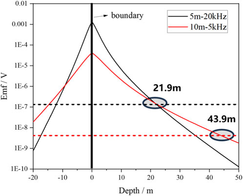
Figure 8. Responses for different spacing–frequency combinations under a DR of 80 dB.

Figure 9 illustrates the DoD distribution under different spacing–frequency configurations, assuming a DR of 80 dB. When only DR is considered, the results indicate that low-frequency, long-spacing configurations markedly enhance DoD, with higher DR providing further improvement. However, this represents an idealized case. When both DR and the signal detection threshold are considered, the maximum DoD shifts from the low-frequency/long-spacing region to moderate spacing and medium frequencies, since signals at extreme low-frequency/long-spacing conditions are already attenuated to the noise floor or below, rendering them impractical to measure. The red contour marks the DoD = 30 m boundary, with spacing–frequency combinations above this line serving as feasible design references. An optimal range of 5–7 m spacing and 10–50 kHz frequency is identified, while the final selection should also consider BHA structural constraints, transmitter power consumption, formation resistivity contrast, and drilling risks.

Figure 9

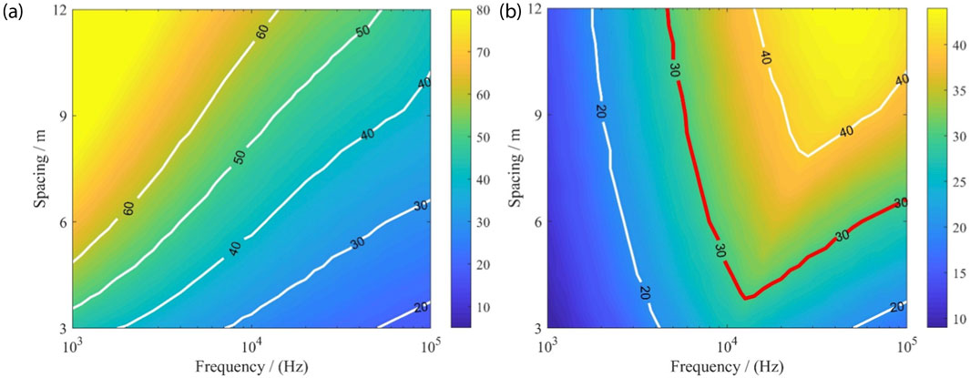
Figure 9. DoD for different spacing–frequency combinations. (a) Considering only dynamic range; (b) considering both dynamic range and noise threshold.

A methodology was developed to characterize the maximum DoD at different resistivity contrasts by jointly considering signal DR and system measurement error. Figure 10 shows Picasso plots of boundary-detection capability for DR values of 70 dB and 80 dB, both incorporating ±5% measurement error, where R1 and R2 denote the resistivities of the current and adjacent layers. For a spacing of 6 m and a frequency of 20 kHz, the results indicate that DoD increases substantially with higher resistivity contrast, whereas low contrast significantly diminishes DoD, making boundary identification challenging. Moreover, increasing DR from 70 dB to 80 dB further improves performance, with the maximum DoD extending from 26.7 m to 36.4 m.

Figure 10

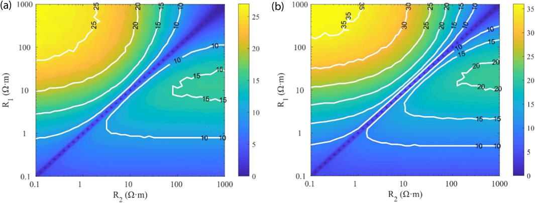
Figure 10. Picasso plots of boundary-detection capability under different resistivity contrasts. (a) DR = 70 dB with ±5% measurement error; (b) DR = 80 dB with ±5% measurement error.

5 Airhang test

To validate the detection capability of the developed UD-AMR tool, an airhang test was conducted. The tool was gradually hoisted above the seawater surface using a crane, while the boundary-detection EMF signal, transmitted by Tc and received by R2, was continuously recorded throughout the lifting process. Figure 11 illustrates the schematic of the equivalent physical model.

Figure 11

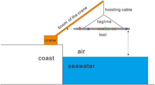
Figure 11. Equivalent model of the airhang test.

Given the extended detection range of ultra-deep EM tools, two key sources of environmental interference were considered during testing: (1) the distance between the tool and the shoreline, and (2) the distance between the tool and the metallic crane arm. Inductive and scattering effects from these structures may distort the measured signals. To ensure the reliability and interpretability of the experimental results, finite element simulations were performed to determine the appropriate test conditions.

The air, seawater and the coast conductivity are set to be 10⁻⁶ S/m, 4 S/m and 10⁻² S/m, respectively. In the simulation, the tool was placed 3 m above the sea surface. The response obtained when the instrument is positioned infinitely far from the coast is used as the reference value. For each case, induced EMF at various distances from the coast are computed, and the relative error is evaluated by comparing the simulated results with the reference. Figure 12 presents simulation results for the effect of shoreline distance on measurement error at 20 kHz and 50 kHz, respectively. When the allowable error threshold is set to 1%, the required shoreline distances are 10.36 m (imaginary part) and 8.95 m (real part) at 20 kHz, and 10.17 m (imaginary part) and 9.88 m (real part) at 50 kHz. These results indicate that maintaining a minimum distance of about 10 m from the coast ensures environmental effects remain acceptable.

Figure 12

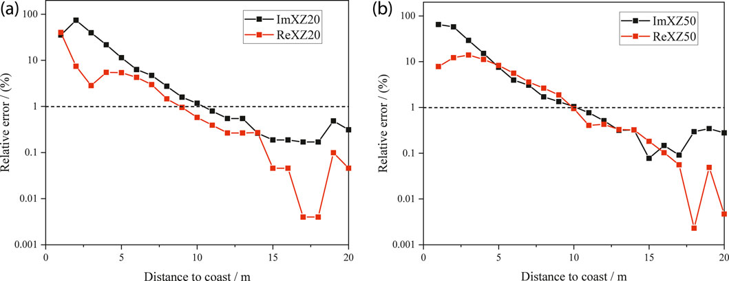
Figure 12. Influence on EMF measurements at different distances to the coast. (a) 20 kHz; (b) 50 kHz.

The influence of the crane boom was also investigated. Figure 13 presents the variation in measured signals as the horizontal distance between the tool and the boom changes. In practice, this distance is affected not only by the tool’s spatial position but also by its orientation relative to the crane, making the interference evaluation more complex. Additionally, the tool’s height relative to the seawater surface influences signal strength: signals are stronger when closer to the surface and weaker when suspended higher. Consequently, the relative contribution of crane interference increases at larger height.

Figure 13

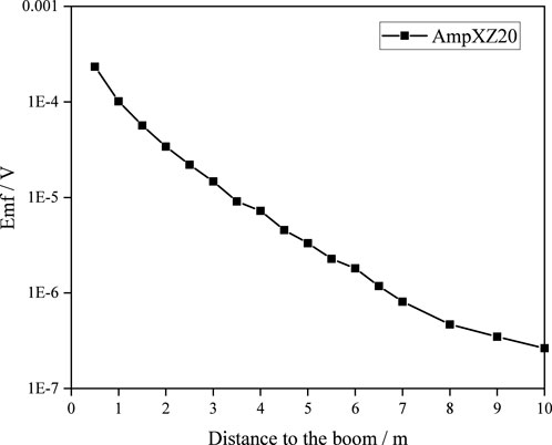
Figure 13. Effect of tool-to-crane boom distance on measured signals.

Therefore, a simplified numerical simulation was conducted to qualitatively assess the influence of the crane boom. The results indicate that the crane exerts a noticeable effect on the measured signals, particularly when the tool is suspended at greater heights. This interference must be carefully considered in both experimental test design and subsequent data interpretation.

Figure 14 compares the boundary-detection EMF amplitudes from both AMR and UD-AMR measurements with numerical simulation results. The air and the seawater conductivity are approximately 10⁻⁶ S/m and 5 S/m, respectively. The simulated responses are plotted as solid lines, while the experimental data are shown as scatter points. They exhibit strong agreement, validating both the modeling methodology and the reliability of the measurements. To ensure consistent comparison, the EMF amplitudes were normalized with respect to the maximum value obtained from the UD-AMR measurements, which was used as the reference for amplitude normalization. Results confirm that both tools successfully detected the seawater interface, however, UD-AMR achieved a significantly greater detection range, exceeding 30 m, which is markedly superior to AMR.

Figure 14

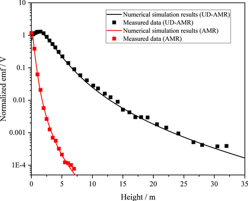
Figure 14. Comparison between experimental and simulated signals for AMR and UD-AMR tools.

Through the optimization of spacing, frequency, and signal dynamic range, the UD-AMR tool achieves significant improvements in depth of detection (DoD) and provides a more robust and reliable solution for formation boundary identification in complex geological structures.

6 Conclusion

This study presents the design, optimization, and validation of a newly developed ultra-deep azimuthal resistivity LWD tool, termed UD-AMR. Comprehensive sensitivity analysis of electromagnetic field components demonstrates that cross-components (e.g., xz and yz) are the most effective for formation boundary detection. Spacing–frequency optimization identified an optimal configuration of 5–7 m spacing and 10–50 kHz operating frequency, achieving a depth of detection (DoD) up to 36.4 m under conditions of 80 dB dynamic range and ±5% measurement error. Air-hang experiments validated the modeling predictions, with measured and simulated results showing strong agreement. The prototype exhibited a maximum boundary-detection range exceeding 30 m, representing a significant improvement over conventional azimuthal resistivity tools.

Beyond validation, the UD-AMR technology shows broad potential for deep and ultra-deep hydrocarbon reservoirs, as well as offshore exploration and development, providing enhanced formation imaging and geosteering capabilities in complex geological environments.

Future work will focus on improving weak-signal detection and processing, temperature-pressure compensation, signal synchronization, and multi-dimensional, multi-interface inversion. Additionally, integrating cloud-edge collaborative computing will be pursued to enable faster downhole data processing and intelligent geosteering. These advancements will further enhance the reliability, adaptability, and imaging performance of ultra-deep EM LWD tools for subsurface characterization.

Data availability statement

The raw data supporting the conclusions of this article will be made available by the authors, without undue reservation.

Author contributions

XY: Writing – original draft, Writing – review and editing. ZY: Writing – review and editing. SH: Writing – review and editing. SD: Writing – review and editing. PQ: Writing – review and editing.

Funding

The authors declare that financial support was received for the research and/or publication of this article. The project is supported by the National Natural Science Foundation of China (Number 42204121) and National Science and Technology Major Project (Number 2025ZD1402102).

Conflict of interest

Authors XY, ZY, and SH were employed by Sinopec Matrix Corporation.

The remaining authors declare that the research was conducted in the absence of any commercial or financial relationships that could be construed as a potential conflict of interest.

Generative AI statement

The authors declare that no Generative AI was used in the creation of this manuscript.

Any alternative text (alt text) provided alongside figures in this article has been generated by Frontiers with the support of artificial intelligence and reasonable efforts have been made to ensure accuracy, including review by the authors wherever possible. If you identify any issues, please contact us.

Publisher’s note

All claims expressed in this article are solely those of the authors and do not necessarily represent those of their affiliated organizations, or those of the publisher, the editors and the reviewers. Any product that may be evaluated in this article, or claim that may be made by its manufacturer, is not guaranteed or endorsed by the publisher.

References

Bell, C., Hampson, J., Eadsforth, P., Chemali, R., Helgesen, T., Meyer, H., et al. (2006). “Navigating and imaging in complex geology with azimuthal propagation resistivity while drilling,” in Proceedings of the SPE Annual Technical Conference and Exhibition (San Antonio, TX: Society of Petroleum Engineers). doi:10.2118/102637-MS

CrossRef Full Text | Google Scholar

Bergeron, J., Rabinovich, M., Murtuzaliyev, M., Ronald, A., and Binyatov, E. (2022). “UDAR: past, present and future—An operator’s experience and perspective on the challenges and opportunities in applications with ultra-deep resistivity tools,” in Proceedings of the SPWLA 63rd Annual Logging Symposium, in Stavanger, Norway (Stavanger, Norway: Society of Petrophysicists and Well Log Analysts). doi:10.30632/SPWLA-2022-0046

CrossRef Full Text | Google Scholar

Bittar, M. S., Rodney, P. F., Mack, S. G., and Bartel, R. R. (1991). “A true multiple depth of investigation electromagnetic wave resistivity sensor,” in Proceedings of the SPE Annual Technical Conference and Exhibition (Dallas, TX: Society of Petroleum Engineers). doi:10.2118/22705-MS

CrossRef Full Text | Google Scholar

Bittar, M. S., Klein, J., Beste, R., Hu, G., Wu, M., Pitcher, J., et al. (2009). A new azimuthal deep-reading resistivity tool for geosteering and advanced formation evaluation. SPE Reserv. Eval. and Eng. 12 (2), 270–279. doi:10.2118/109971-PA

CrossRef Full Text | Google Scholar

Hartmann, A., Vianna, A., Maurer, H. M., Sviridov, M., Martakov, S., Lautenschläger, U., et al. (2014). “Verification testing of a new extra-deep azimuthal resistivity measurement,” in Proceedings of the SPWLA 55th Annual Logging Symposium, in Abu Dubai, UAE (Society of Petrophysicists and Well Log Analysts).

Google Scholar

Holmquist, A. N., Khemissa, H., Agnihotri, P., and Augustine, A. (2025). “Novel multi-dimension inversion of ultra-deep azimuthal resistivity service allows strategic decision in real-time enhancing reservoir management,” in Proceedings of the GOTECH (Abu Dubai, UAE). doi:10.2118/224537-MS

CrossRef Full Text | Google Scholar

Huang, M., and Yang, Z. (2020). Simulation to determine depth of detection and response characteristics while drilling of an ultra-deep electromagnetic wave instrument. Pet. Drill. Tech. 48 (1), 114–119. doi:10.11911/syztjs.2019132

CrossRef Full Text | Google Scholar

Ma, J., Riofrio, K., Clegg, N., Sinha, S., Wu, H., Kotwicki, K., et al. (2022). “Successful geostopping using a recently developed LWD look-ahead ultra-deep EM resistivity tool,” in Proceedings of the SPE Annual Technical Conference and Exhibition (Abu Dhabi, UAE: Society of Petroleum Engineers). doi:10.2118/211613-MS

CrossRef Full Text | Google Scholar

Omeragic, D., Li, Q., Chou, L., Yang, L., Duong, K., Smits, J., et al. (2005). “Deep directional electromagnetic measurements for optimal well placement,” in Proceedings of the SPE Annual Technical Conference and Exhibition (Dallas, TX: Society of Petroleum Engineers). doi:10.2118/97045-MS

CrossRef Full Text | Google Scholar

Rodney, P. F., Meador, R., Rondney, P. F., and Thompson, L. W. (1983). “The electromagnetic wave resistivity MWD tool,” in Proceedings of the SPE Annual Technical Conference and Exhibition (San Francisco, CA: Society of Petroleum Engineers). doi:10.2118/12167-PA

CrossRef Full Text | Google Scholar

Salim, D., Chen, Y. H., Liang, L., Denichou, J. M., Cunha, A. M., Roberto, S. A., et al. (2025). “Case study of active resistivity ranging with ultra-deep azimuthal resistivity measurements while drilling,” in Proceedings of the SPWLA 66th Annual Logging Symposium, in Abu Dubai, UAE (Society of Petrophysicists and Well-Log Analysts). doi:10.30632/SPWLA-2025-0125

CrossRef Full Text | Google Scholar

Seydoux, J., Legendre, E., Mirto, E., Dupuis, C., Denichou, J. M., Bennett, N., et al. (2014). “Full 3D deep directional resistivity measurements optimize well placement and provide reservoir-scale imaging while drilling,” in Proceedings of the SPWLA 55th Annual Logging Symposium, in Abu Dhabi, UAE (Society of Petrophysicists and Well Log Analysts).

Google Scholar

Singh, M., Thakur, P. D., Al Baloushi, M. N. M., Saadi, H. A., Mansoori, M. M., Mesafri, A. S., et al. (2021). “Real-time 3D ultra-deep directional electromagnetic LWD inversions: an innovative approach for geosteering and geomapping water slumping movement around sub-seismic fault, onshore in Abu Dhabi, UAE” in Proceedings of the SPE Annual Technical Conference and Exhibition (Society of Petroleum Engineers). doi:10.2118/207478-MS

CrossRef Full Text | Google Scholar

Wang, L., Qiao, P., Li, Z. Q., Zhang, P., Deng, S., and Fan, Y. (2023a). A new semianalytical algorithm for rapid simulation of triaxial electromagnetic logging responses in multilayered biaxial anisotropic formations. Geophysics 88 (2), D115–D129. doi:10.1190/geo2021-0714.1

CrossRef Full Text | Google Scholar

Wang, L., Qiao, P., Zhao, W. N., Cao, F., and Fan, Y. (2023b). A new propagator matrix algorithm to compute electromagnetic fields in multilayered formations with full anisotropy. IEEE Trans. Geoscience Remote Sens. 61, 1–11. doi:10.1109/TGRS.2023.3302513

CrossRef Full Text | Google Scholar

Wang, L., Wu, K. K., Liu, Y. M., Xu, X. K., Deng, S. G., and Qiao, P. (2025). Focusing mechanism and anisotropy correction of array induction logging responses for shale reservoirs in horizontal wells. Petroleum Sci. doi:10.1016/j.petsci.2025.08.009

CrossRef Full Text | Google Scholar

Wu, H. H., Golla, C., Parker, T., Clegg, N., and Monteilhet, L. (2018). “A new ultra-deep azimuthal electromagnetic LWD sensor for reservoir insight,” in Proceedings of the SPWLA 59th Annual Logging Symposium, London, United Kingdom (Society of Petrophysicists and Well Log Analysts).

Google Scholar

Wu, B., Yang, Z., Guo, T., and Yuan, X. (2022). Response characteristics of logging while drilling system with multi-scale azimuthal electromagnetic waves. Pet. Drill. Tech. 50 (6), 7–13. doi:10.11911/syztjs.2022107

CrossRef Full Text | Google Scholar

Wu, M., Wu, D., Ma, J., Yan, T., Lozinsky, C., and Bittar, M. (2024). “Enhancing local anisotropy characterization with ultra-deep azimuthal resistivity measurements,” in Proceedings of the SPWLA 65th Annual Logging Symposium, in Rio de Janeiro, Brazil (Society of Petrophysicists and Well-Log Analysts). doi:10.30632/SPWLA-2024-0070

CrossRef Full Text | Google Scholar

Yang, Z., Yang, J., and Han, L. (2013). Numerical simulation and application of azimuthal propagation resistivity imaging while drilling. J. Jilin Univ. Earth Sci. Ed. 43 (6), 2035–2043. doi:10.13278/j.cnki.jjuese.2013.06.023

CrossRef Full Text | Google Scholar

Yang, Z., Yang, J., Han, L., and Li, C. (2016). Interface detection performance analysis of azimuthal electromagnetic while drilling. Acta Pet. Sin. 37 (7), 930–938. doi:10.7623/syxb201607012

CrossRef Full Text | Google Scholar

Yuan, X., Deng, S., Li, Z., Han, X. M., and Hu, X. F. (2022). Deep-detection of formation boundary using transient multicomponent electromagnetic logging measurements. Petroleum Sci. 19 (3), 1085–1098. doi:10.1016/j.petsci.2021.12.016

CrossRef Full Text | Google Scholar

Yue, X., Liu, T., Li, G., Li, G., Nie, Z., Ma, M., et al. (2022). An analytically fast forward method of LWD azimuthal electromagnetic measurement and its geo-steering application. Chin. J. Geophys. 65 (5), 1909–1920. doi:10.6038/cjg2022P0233

CrossRef Full Text | Google Scholar