Estimating the density of individual particles from the settling of a particle cloud

The density of individual particles is commonly assessed experimentally by quantifying the settling velocity of a collection of particles transferred into a settling column and allowed to settle under the action of gravity. The individual settling velocities of the particles are recorded close to the bottom of the settling column, in a region where it is assumed that the particles have reached their Stokes terminal velocity after the particle cloud has broken up. In the present study we use numerical particle-based simulations in the Stokes regime to demonstrate that this fundamental assumption might not be fulfilled in practice. Even at low volume fraction of monodisperse spheres, a large deviation from the Stokes settling velocity was found. In the case of a collection of polydisperse spheres, a distinction could be made between particles belonging to a cloud, and particles trailing the cloud. It was found that the velocity of the largest trail particles is reasonably close to their Stokes settling velocity. However, the particles close to the core of the cloud can have velocities more than ten times their Stokes velocities, making the use of the single-particle Stokes velocity based on the core particle not suitable to extract the particle density without corrections. An expression based on the local volume fraction, the cloud radius and the particle settling velocity in the cloud is proposed to estimate the single-particle Stokes settling velocity, and therefrom the particle density.

1 Introduction

Stokes settling velocity of small micro-particles is one of the main input parameters of the numerical models used to estimate the transport of these particles in the water column (Lesser et al., 2004; Blumberg et al., 1996; Normant, 2000). The quantification of particle settling velocities is therefore a major topic in marine sciences, as it enables the prediction of the transport and fate of marine sediments in estuaries, seas and oceans (Rulent et al., 2024; Masria et al., 2024; Zhang and Choi, 2025; Isachenko and Chubarenko, 2022). Recently, a lot of research has focused on the microplastics found in water bodies (Ahmed et al., 2021; Hale et al., 2020; Andrady, 2011; Li et al., 2018), and this has similarly led to numerous studies to measure the settling velocities of microplastics (Al-Zawaidah et al., 2024; Yu et al., 2022; Dittmar et al., 2023; Dittmar et al., 2024; Goral et al., 2023; Zhang et al., 2023). In aquatic environment, most of the suspended particulate matter (SPM) is in the form of flocs (Chassagne and Safar, 2020; Manning et al., 2010; Spencer et al., 2022; Gu et al., 2025). Flocs are composed of mineral clay particles (and/or other small colloidal particles such as microplastics) bound by organic matter (often in the form of polymeric substances). One particular property of flocs is that their density is variable, as it depends on their composition (Chassagne et al., 2021; Deng et al., 2019; Safar et al., 2022). Knowing the size of a floc is therefore not enough to estimate its density as it would be for mineral particles, for example, (which have densities in the range of 2,600 ${\mathrm{k}\mathrm{g}/\mathrm{m}}^3$). From in-situ observations, only particle sizes can be assessed, and therefore complementary measurements are required to estimate their density, which is done by recording their settling velocity.

The most common approach is to sample particles in the field and study them on board the ship or in the laboratory upon return. A small amount (mL) of the collected suspension (water + particles) is transferred into a settling column containing water with the same properties as the sampling area (same chemical properties, same temperature). A detailed description is given in (Ali et al., 2024). The settling velocity is recorded with a camera at locations far away from the injection point, to ensure that the particles have reached their terminal velocities (Ali et al., 2024; Manning et al., 2011; Manning, 2015; Fall et al., 2021; Kaiser et al., 2019; Khatmullina and Chubarenko, 2021; Glockzin et al., 2014). In most practical cases involving flocs, particle (floc) density is very close to the density of the suspending liquid, typically water. Therefore, the particles have reached their terminal velocity and are expected to settle in the Stokes regime when reaching the recording point. In the Stokes regime, the settling velocity $u$ of an isolated particle in an unbounded domain is proportional to the solid-fluid density difference $\mathrm{\Delta }\rho$ according to $u=(2/9)\mathrm{\Delta }\rho g{a}^2/\mu$, where $\mu$ is the fluid viscosity, $g$ is the acceleration of gravity, and $a$ is the radius of the particle. The density difference between particle and water is given by $\mathrm{\Delta }\rho ={\rho }_p-{\rho }_w$.

Recent experiments with flocs have shown that the settling velocity measured with the settling column method is incompatible with predictions using realistic values of the floc density (Ali et al., 2024). Measurements done by transferring a drop of a dilute suspension of flocs at the top of the column give values of the settling velocity of flocs at the bottom of the column that are much larger than the value predicted by the Stokes settling rate. One of the reasons for this large velocity is that flocs fall in the wake of others, which enhance their settling velocity. This velocity was hence termed “collective settling” velocity in (Ali et al., 2024). Experiments shown in the same article have instead demonstrated that dropping single flocs in the settling column gave settling velocities (“individual settling”) that are close to the Stokes settling value.

The results of this study on the effect of collective motions on particle settling is of practical interest in several contexts. Collective settling is encountered during the discharge of particle-laden plumes in (deep-sea) mining (Peacock and Ouillon, 2023), the propagation of turbidity currents (Meiburg and Kneller, 2010), hypopycnal plumes (Snyder and Hsu, 2011), etc. To estimate the settling fluxes in the far-field region of the plume, where the particle concentration is very low, the Stokes settling velocity is used as input parameter, and its validity assumed. The assumption is based on the fact that the suspension is very dilute (volume fraction within 1%), so hydrodynamic interactions are assumed to be unimportant. The current study challenges this assumption.

In this article, we start from experimental observations using spherical particles of given size and density. The use of such well controlled particles enables us to be in the regime where the Stokes formula is known to hold exactly in the individual settling case and avoid the uncertainties in shape, size and density encountered when using flocs. Experiments were performed using a video microscopy setup described in Section 2, quite similar to the ones used by other experimentalists (Manning et al., 2011; Manning, 2015; Fall et al., 2021; Kaiser et al., 2019; Khatmullina and Chubarenko, 2021; Glockzin et al., 2014). We then interpret the experimental results using numerical simulations that illustrate the difference between collective settling and individual settling. Settling of suspension drops in quiescent viscous liquids has been studied both experimentally and numerically (Nitsche and Batchelor, 1997; Ekiel-Jeżewska et al., 2006; Metzger et al., 2007). In these studies, the initial velocity of the cloud, breakup of the cloud and particle leakage from the cloud were the main focuses. In the current article, we are interested in discussing implications of theoretical predictions for the settling velocity as a function of solid concentration and particle polydispersity in size in view of experimental measurements. The simulations presented in Section 3 enable to propose a simple expression for the single-particle Stokes settling velocity and density using the local volume fraction, the cloud radius and the particle settling velocity in the cloud. This expression is valid for a dilute suspension and a cloud size much larger than the particle’s size, which are conditions generally fulfilled in the experiments.

2 Experimental methods

For the settling experiments two batches of polystyrene particles are utilized, with a median particle diameter of approximately 600 $\mathrm{\mu }\mathrm{m}$ and 900 $\mathrm{\mu }\mathrm{m}$, as characterized by the particle size distribution shown in Figure 1 (obtained with a Malvern Mastersizer 2000 set-up described in (Ali and Chassagne, 2022)). The density of the particles is in the range of $1020-1040$ ${\mathrm{k}\mathrm{g}/\mathrm{m}}^3$. The solvent used is water (density ${\rho }_w=1000$ ${\mathrm{k}\mathrm{g}/\mathrm{m}}^3$).

Figure 1

Figure 1. (a) Particle size (diameter) distribution of polystyrene particles as measured by Malvern Mastersizer 2000. (b) Schematic representation of the FLOCCAM setup (Ali et al., 2022).

The settling velocity was measured with a home-made video microscopy device (FLOCCAM) designed to measure particle size distributions (PSDs) for particles larger than 20 $\mathrm{\mu }\mathrm{m}$ and their respective settling velocities (Ali et al., 2022; Al et al., 2022; Ye et al., 2020; Manning et al., 2007; Ali et al., 2024). A schematic of the setup is shown in Figure 1.

The FLOCCAM system consists of a rectangular settling column measuring $10\mathrm{c}\mathrm{m}\times \mathrm{10}\mathrm{c}\mathrm{m}\times \mathrm{30}\mathrm{c}\mathrm{m}$, with glass panels on the front and back, and plastic side walls. Video footage of the settling particles is captured by a 5 MP CMOS camera with a resolution of $2592\times 2048$ pixels and a pixel size of 4.8$\mathrm{\mu }\mathrm{m}$. The camera, equipped with a Global Shutter (model: iDS UI-3180CP-M-GL Rev.2.1, AB02546), is paired with a telecentric lens (model: S5VPJ2898) manufactured by Sill Optics GmbH and Co. KG, featuring an adjustable working distance and a C-mount. This combination provides a pixel resolution of approximately 8.6$\mathrm{\mu }\mathrm{m}$.

For illumination, a Flat Lights TH2 Series Red LED panel (63 $\mathrm{m}\mathrm{m}\times$ 60 $\mathrm{m}\mathrm{m}$) was employed due to its high directivity, ensuring consistent lighting throughout the experiments. The light panel was powered and controlled by a DC 24V Input Controller (model: PB-2430-1) from CCS Inc.

To inject the particles into the settling column, a plastic conical feed well terminating with a rectangular outlet measuring 2 $\mathrm{m}\mathrm{m}\times \mathrm{10}\mathrm{m}\mathrm{m}$ was used. A suspension drop containing particles was carefully extracted using a pipette and released into the column. Settling velocities were recorded approximately 25 $\mathrm{c}\mathrm{m}$ below the injection point.

The post-processing of FLOCCAM videos was done by using the software Safas (Ali et al., 2022; MacIver, 2019). Safas, which stands for Sedimentation and Floc Analysis Software, is a Python module specifically designed for processing and analyzing images and videos of sedimenting particles, especially cohesive sediment flocs. This open-source software enables users to easily extract critical data such as particle size, morphology, and settling velocity, allowing users to customize its image filters.

In the first set of experiments, particles with a given size (600 $\mathrm{\mu }\mathrm{m}$ or 900 $\mathrm{\mu }\mathrm{m}$) were tested under both individual settling and group settling conditions. For the individual settling case, each particle was introduced into the settling column one at the time, ensuring no interference from neighbouring particles. In the collective settling case, a few mL suspension containing particles were transferred into the column.

The group settling behaviour of a polydisperse group of particles, consisting of a mixture of 600$\mathrm{\mu }\mathrm{m}$ and 900$\mathrm{\mu }\mathrm{m}$ particles, was also studied and compared to the individual settling behaviours of particles from each size range. The ratio between the number of 600 $\mathrm{\mu }\mathrm{m}$ and 900 $\mathrm{\mu }\mathrm{m}$ particles in the mixed group is $7:1$.

3 Simulation approach

Simulations were carried out with a Stokesian dynamics method in the force formulation (Durlofsky et al., 1987; Brady and Bossis, 1988). The simulation code is the same as in Ref. (Li and Botto, 2024), where complete validation cases are presented. Essentially the method is based on calculating the average settling velocity starting from the particle position by knowing that, in a low-Reynolds number suspension, the velocity of each particle is a linear function of the gravitational forces (weight and buoyancy) acting on each particle.

The numerical simulations are carried out as follows. Firstly, particles are randomly placed inside a cubic box ensuring no overlap between any pair of particles. The group of particles in the box is assumed to settle in an unbounded fluid. Then, the particle velocities are calculated by the Stokesian dynamics method (Durlofsky et al., 1987; Brady and Bossis, 1988). In the Stokesian Dynamics method, a mobility matrix $\mathbf{M}$ is assembled based on the relative position of all the particles. For this matrix, which incorporates the hydrodynamic interactions between the particles, we adopt the Rotne-Prager approximation (Rotne and Prager; Zuk et al., 2014) (this approximation is appropriate for dilute suspensions). Formulas for the components of $\mathbf{M}$ in this approximation are taken from Refs. (Rotne and Prager; Zuk et al., 2014). The vector containing the velocities of the particles is calculated from the following equation:

$\mathbf{U}=\mathbf{M}\mathbf{F},(1)$

where $\mathbf{U}$ is a $3N\times 1$ vector of the velocities of the $N$ particles, and $\mathbf{F}$ is a $3N\times 1$ vector of the forces on the $N$ particles. For a particle with radius $a$, the force on the particle is $\mathbf{f}=\frac{4\pi a^3}{3}({\rho }_p-{\rho }_w)\mathbf{g}$, where ${\rho }_p$ and ${\rho }_w$ are the densities of the particle and water, respectively, and $\mathbf{g}$ is the gravitational acceleration. In the simulations, the instantaneous particle settling velocities are calculated according to Equation 1, with forces corresponding to the assigned random configuration of the particles.

When the average separation between identical particles of radius $a$ is infinitely large, $\mathbf{M}$ is a diagonal matrix with entries equal to the mobility coefficient $1/(6\pi \mu a)$, where $\mu$ is the viscosity of water. At finite interparticle separations, interparticle interactions alter the settling velocity of each particle, and can result in the average settling velocity of a group of particles being smaller or larger than the Stokes settling velocity. The average settling velocity of a particle is $⟨\mathbf{U}⟩=\frac{4\pi a^3}{3}({\rho }_p-{\rho }_w)⟨\mathbf{M}⟩\mathbf{g}$, where $⟨\mathbf{M}⟩$ depends on the interparticle separation or, equivalently, on the solid volume fraction. For a polydisperse suspension, each size class will have its own average settling velocity (Li and Botto, 2024).

The simulation results are presented in non-dimensional form. The simulations are non-dimensionalized using a characteristic length $a_0$ and a characteristic Stokes velocity $u_0=\frac{2a_0^2}{9\mu }({\rho }_p-{\rho }_w)g$. For the polydispersed simulation, the characteristic length is the average radius of the size distribution $⟨a⟩$.

4 Results and discussions

4.1 Experimental results

Figure 2 (top) presents the results of a settling experiment for particles of diameters centered around 600$\mathrm{\mu }\mathrm{m}$, comparing individual and collective settling. When particles were introduced individually into the settling column, their velocities followed reasonably well Stokes’s formula for ${\rho }_p\simeq \mathrm{1030}\mathrm{k}\mathrm{g}/{\mathrm{m}}^{\mathrm{3}}$ (blue dots), with a small dispersion about this law.

Figure 2

Figure 2. (top) experimental particle settling velocities, comparing individual and group settling for a range of particle diameters centered at 600$\mathrm{\mu }\mathrm{m}$; (bottom) experimental particle settling velocities for a predominantly bi-disperse mixture of 600$\mathrm{\mu }\mathrm{m}$ and 900$\mathrm{\mu }\mathrm{m}$.

Having particles settling in a group has several effects: a larger spread in velocities and a larger average velocity are found for a given diameter in the collective settling case (orange dots) compared to the individual settling case (blue dots). Note that the FLOCCAM setup does not allow to measure velocities larger than $8.5\mathrm{m}\mathrm{m}/\mathrm{s}$, which explains the cut-off observed in Figure 2. Another effect is that when multiple particles are in the field of view, the software clearly has issues (related to grayscale definition) to correctly estimate particle sizes, leading to the observed spread in size.

Figure 2 (bottom) represents the comparison between individually settling particles and suspensions containing both particles with diameters 600$\mathrm{\mu }\mathrm{m}$ and 900$\mathrm{\mu }\mathrm{m}$, with a ratio of small to large sizes of 7:1. The presence of 900$\mathrm{\mu }\mathrm{m}$ particles in the suspension causes a significant increase in the velocity distribution of the 600$\mathrm{\mu }\mathrm{m}$ particles, compared to the group settling behavior shown in Figure 2 (top) and to a notable increase in the settling velocity of the 900$\mathrm{\mu }\mathrm{m}$ particles compared to the case where they were sampled individually. Again, due to the cutoff at $8.5\mathrm{m}\mathrm{m}/\mathrm{s}$, it was not possible to record particles settling at a higher velocity, but from the data it is clear that more particles are settling at higher velocities in Figure 2 (bottom) than in Figure 2 (top). The distinction between 600$\mathrm{\mu }\mathrm{m}$ and 900$\mathrm{\mu }\mathrm{m}$ particles in Figure 2 (bottom) is also somewhat arbitrary, as the size determination by the software is problematic due to the calibration of the grayscale.

From the experiments, it can be concluded that, in line with what has been observed with flocs, a large spread in sizes and velocities is obtained during the collective motion of particles, even though these particles have a density close to water and settle in the Stokesian regime (Ali et al., 2024).

The increase in the number of particles in a suspension is generally believed to give a reduction in settling rate (Brzinski and Durian, 2018), a phenomenon commonly referred to as hindered settling. In our experiment instead we have a case of enhanced settling. The reason lays in the fact that particles in the FLOCCAM experiment are settling in a group, in a water otherwise devoid of particles, as sketched in Figure 3a. In that simplistic sketch, it is assumed that the particles fall collectively with the same velocity. Their velocity can be estimated, using Stokes, as being equal to the velocity of the cloud, i.e., $\mathbf{u}=\frac{2R^2}{9\mu }({\rho }_R-{\rho }_w)\mathbf{g}$ where ${\rho }_R=\varphi {\rho }_p+(1-\varphi ){\rho }_w$ is the density of the cloud of radius $R$, $\varphi =N{(a/R)}^3$ is the volume fraction of particles of radius $a$ inside the cloud and $N$ is the number of particles inside the cloud. This leads to $u/u_0=N$, where $u_0$ is the single particle Stokes velocity. A better formulation has been derived by Hadamard and Rybczynski, who accounted for the fact that the fluid velocities at the cloud/solvent interface are continuous (Chassagne, 2021), yielding

$u/u_0=1+N\frac{6a}{{\lambda }^{*}R}(2)$

where $\lambda *$ is drag force parameter ranging from $\lambda *=5$ (dilute cloud) to $\lambda *=6$ (concentrated cloud). It is clear from this equation that the velocity of a particle in the cloud is much larger that the Stokes settling velocity of an individual particle.

Figure 3

Figure 3. Sketches showing (a) collective settling of particles, and (b) hindered settling of a suspension. Blue lines with arrows represent the fluid streamlines, and red arrows show the particle moving direction. $l=2R$ is the size of the particle group (i.e., the diameter of the gray dashed circle enclosing the particles in (a)), and $L$ is the lateral size of the container.

In hindered settling, the group of particles spans the entire width of the tank (Figure 3b). In this latter case hydrodynamic interactions produce a significant upward flow by conservation of volume (the flux of particles moving downward imposes a water flux upward). This results in a reduction of individual particle settling velocities (Chassagne, 2021).

We will now proceed to analyze in more detail the kinetics of collective settling using numerical simulations.

4.2 Settling of two spheres

In order to get a first estimate of characteristic lengths, we consider the settling kinetics of pairs of spheres. We first study the classical case of a pair of identical spherical particles of radius $a_1=a_2=a$ (red line and symbols in Figure 4). It is well-known that their settling velocity increases as the center-to-center separation $r$ between the particle centers decreases, and is larger than the settling velocity of each particle by a factor that reaches almost $50\%$ at close separation for spheres that are horizontally aligned, as illustrated in Figure 4. The hydrodynamic influence of one sphere on the other sphere decays slowly, as $1/r$, therefore, to reach values comparable to the single-particle settling velocity one should have separations $r\approx 10a$. For an homogeneous system, an interparticle separation of $r\approx 10a$ corresponds to a very small solid volume fraction of $0.1\%$, so one should have local volume fractions that are extremely small for the influence of hydrodynamic particle-particle interactions to be negligible. The rule of thumb of 10 particle radii needs to be modified when the pair comprises spheres of dissimilar size. For example, by examining the case $a_2/a_1=0.25$ described by the blue line and symbols in Figure 4, we can see that for a separation $2r/(a_1+a_2)=20$ the settling velocity of particle 2 has not yet converged to its own Stokes settling velocity. This despite the fact that $2r/(a_1+a_2)=20$ and $a_2/a_1=0.25$ yields a large separation of $r=50a_2$.

Figure 4

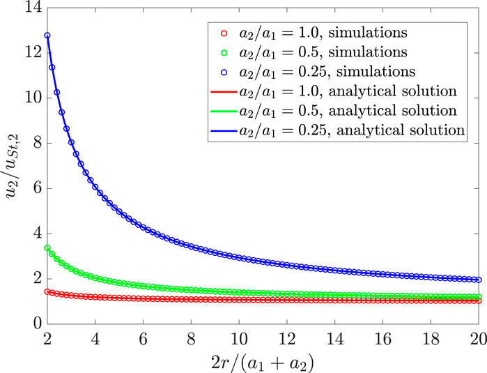
Figure 4. Simulated settling velocities of a sphere of radius $a_2\le a_1$ in a simulation of a horizontally aligned sphere pair, where one of the spheres has a radius $a_1$ and the other has a radius $a_2$. $u_{St,2}$ is the Stokes velocity of the sphere with radius $a_2$ and $r$ is the center-to-center distance of the pair. Lines are the analytical solutions of Ref (Wacholder and Sather, 1974).

4.3 Settling of a group of spheres

The long-range velocity hydrodynamic disturbances created by particles settling in a group result in settling velocities that are much larger than the single particle settling velocity, but also to a significant spread in velocity. In Figure 5 we compare group settling and individual settling for configurations in which 100 particles are randomly placed in a cubic box of side $L=35a$. In this plot, the average separation is such that the volume fraction is $1\%$ and the average velocity of the group is more than 6 times larger than the single-particle Stokes velocity. The average velocity of the group will depend on the (local) volume fraction, therefore in Figure 6 we plot the average velocity of the group of particles as a function of $\varphi$, where $\varphi$ is the volume fraction of particles inside the cloud. This plot is obtained by fixing the size of the cloud and the simulation box and changing the number of particles. To plot the dashed line in Figure 6, the radius of the cloud, $R$, is chosen as half of the box size $L/2$. From these graphs we can see that the dispersion around the mean value for these monodisperse simulations is comparatively small. An analysis of the problem of randomly distributed point-forces located within a sphere of radius $R$ in Ref. (Ekiel-Jeżewska et al., 2006). reports fluctuating velocity of at most $5\%$ of the difference between the average velocity of the particle group and the single particle settling rate. This is due to the fact that particles in the center of the group move with a velocity comparable to the average velocity of the group, while the settling velocity of particles at the group’s periphery is smaller than that of the group (see Figure 7a). The average velocity of the group follows approximately the expression, derived by Ekiel-Jeżewska and co-workers (Ekiel-Jeżewska et al., 2006):

$⟨u⟩/u_0=1+\frac{6}{5}\left(\frac{R^2\varphi }{a^2}-\frac{a}{R}\right)(3)$

This expression can be used for an estimation of the settling velocity of particles in a dilute cloud. Note that Equations 2, 3 reduce to the same expression, $1+\frac{6}{5}\frac{R^2\varphi }{a^2}$, for large $R/a$.

Figure 5

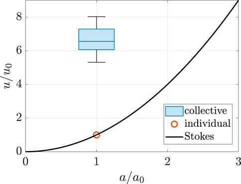
Figure 5. Monodisperse case: Particle settling velocities normalized by the particle Stokes settling velocity as function of the normalized particle size. Single particles settle according to Stokes (red circle), whereas particles settling collectively display a spread in settling velocities (boxplot). The mean value and standard deviation of the settling velocity are 6.6 and 0.7, respectively. The horizontal line in the blue box represents the median value. The volume fraction of particles is $1\%$ and 100 particles are used in the simulation. The radius of the cloud is half of the box size.

Figure 6

Figure 6. Monodisperse case: average particle settling velocity normalized by the individual Stokes settling velocity versus volume fraction in the settling group. Symbols are results of current simulations with error bars showing the standard deviation of the particle velocity fluctuations. The dashed line is the analytical solution from the reference (Ekiel-Jeżewska et al., 2006) for particles randomly distributed within a spherical cloud. The radius of the cloud is half of the box size.

Figure 7

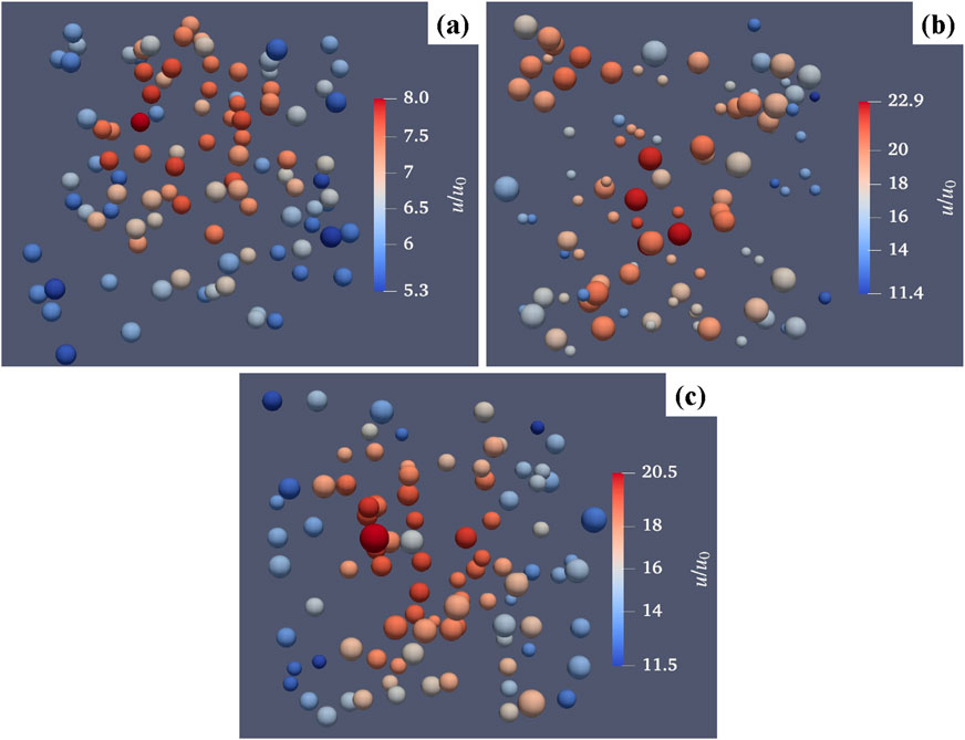
Figure 7. Example of simulated configurations for (a) monodisperse, (b) bidisperse and (c) polydisperse cases. The particles are colored according to their settling velocities (normalized by the reference Stokes velocity).

4.4 Settling of a bidisperse group of spheres

We now turn to the analysis of simulations in the bidisperse case. The normalized particle settling velocities in both individual settling and group settling cases are shown in Figure 8. For these calculations, in the individual settling case, a single particle with radius $a_1$ or $a_2$ is placed inside the domain. For collective settling, 50 small particles with radius $a_1$ and 50 large particles with radius $a_2$ are placed inside a cubic box with size $L=58a_1$, resulting a volume fraction as 0.01. At this volume fraction, in the collective settling, the settling velocities of the small particles range from 10 times to 20 times their Stokes velocity (the mean value and standard deviation of the settling velocity as 16.4 and 2.3, respectively). This large influence of bidispersity on the average settling rate can be understood from the fact that, as shown in Figure 4, in a pair of dissimilarly sized particles the velocity of the small particle is larger than its Stokes settling velocity and approaches the velocity of the large particle as $r$ is reduced (in a very dilute dispersion of particles, hydrodynamic interactions are essentially pair-wise additive, so results for particle pairs translate qualitatively to a particle cloud). Of course, in a bidisperse situation the larger particles will settle faster than the small particles, resulting in phenomena of segregation within an initially homogeneous cloud (Faletra et al., 2015) or even disintegration of the cloud (Ho et al., 2016) depending on the relative particle size.

Figure 8

Figure 8. Bidisperse case: Normalized particle settling velocities for collective and individual settling. For the collective settling, 50 particles of radius $a_0$ were mixed with 50 particles of radius $2a_0$. The box plot represents the velocity distribution of each size class in the mixture.

4.5 Settling of a polydisperse group of spheres

Finally, Figure 9 shows results for the polydisperse case. The particle size is distributed according to a Gaussian with mean 1.5 and standard deviation 0.2. A graph comparing the settling velocity vs. particle radius for individual settling and collective settling is shown in Figure 9a. For the collective settling simulation, 100 particles are placed randomly in a cubic box with $L=50$ (volume fraction $\varphi =0.01$). The average settling velocity of the group of particles is at least 10 times larger than the individual settling rate. Fluctuations in the velocity around the mean value, for each value of $a$ are comparatively large, so assigning a law of dependence between $u$ and $a$ can only be done in a least-square sense. The scatter plot of Figure 9a and the values presented in Figure 9b, where the settling data is plotted per particle size classes, indicate that in group settling the correlation between particle size and velocity is weak. It may therefore seem that estimating the particle Stokes settling velocity (and hence density) for a polydisperse suspension is not as straightforward as for a suspension of monodisperse particles, where Equations 2, 3 can be used. However, we will now see that another effect, typical of suspensions of polydisperse particles, in fact helps.

Figure 9

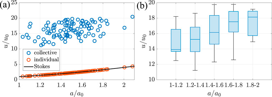
Figure 9. Polydisperse case: (a) normalized particle settling velocities comparing collective and individual settling, and (b) spread of the normalized particle settling velocities per size range during collective settling.

When a cloud of spherical monodisperse particles settles, the cloud maintains its shape while growing in size until it breaks up into “blobs”, except for clouds with very low initial volume fractions which disintegrate without keeping their shapes. A polydispersity in size has the effect of destabilising the cloud much faster. If the polydispersity is large, the cloud disintegration is faster.

In Figure 10a we show a snapshot of a dynamic simulation of a polydisperse suspension of 949 particles initially confined within a sphere. The initial volume fraction is $1\%$. The particle sizes are distributed according to the discrete logarithmic size distribution shown in Figure 10b. Because of the large polydispersity (the parameter $\sigma$ characterising the log-normal is 0.32, while the mean radius is 0.94) the initial spherical cloud has lost its coherence in shape in a comparatively short time. The cloud has disintegrated, leaving a trail of small particles (seen at the top of the image) that settle with a velocity still larger than their Stokes velocity. The larger particles near the bottom experience hydrodynamic interactions and settle at a velocity much larger than the Stokes velocity.

Figure 10

Figure 10. (a) A snapshot of a dynamic simulation of a settling polydisperse cloud. Particles are colored according to their sizes. (b) Particle size distribution used in the dynamic simulation. The mean value and standard deviation of the particle radius is 0.94 and 0.32, respectively.

Particles in the tail reach their Stokes settling velocity as time progresses. This trend is demonstrated in Figure 11, where the particle velocities are given in terms of trail particles (in red) and particles in the core of the cloud (blue) for $\varphi =1\%$. If the distance between a particle and the average position of all the particles is larger than the radius of the initial cloud, this particle is considered as a trail particle. Otherwise it is considered as in the cloud. The red circles come closer to the Stokes velocity line in time. The figure also shows that the largest (heaviest) particles in the trail offer the best agreement with the Stokes velocity. This is because the hydrodynamic influence of the smallest particles in a polydisperse distribution on the large particles is relatively weak (Li and Botto, 2024). The small particles “feel” the influence of the large particles, but not vice versa. This also explains why in the experiments of Ali et al. (Ali et al., 2024) the estimation of the effective density of the smallest flocs had a larger variance for the small flocs than for the large flocs. From Figure 11 it is also apparent that the velocity of the particle belonging to the core of the cloud is almost independent of the particle size, something also found experimentally.

Figure 11

Figure 11. Particle velocities for different size classes at three different times in the dynamic simulation. Blue symbols are for the particles in the cloud, red symbols are for the particles in the trail, and the red lines are the Stokes velocities. Time progresses from (a–c). (a,b) happen before the cloud is completely broken, and (c) happens after that.

4.6 Criteria for stability of polydisperse cloud of particles

The time for disintegration of a particle cloud depends primarily on the initial volume fraction. For example, for $\varphi =0.01\%$ and $\varphi =0.001\%$ no typical cloud evolution behaviour (with a toroidal vortex) is observed in our dynamic simulations, regardless of the number of particles in the cloud. For $\varphi =0.1\%$, the evolution follows initially a typical cloud behavior for $N=250$ until the cloud disintegrates. For monodisperse particle clouds, Ho et al. (2016) found that the cloud breakup time is in the range $500-1200{\tau }_c$, where ${\tau }_c=R_0/⟨u⟩$ is the time it takes for a spherical cloud of radius $R_0$ to travel a distance $R_0$ when moving with a velocity $⟨u⟩=4/15\varphi \mathrm{\Delta }\rho g{R}^2/\mu$ (equal to Equation 3 when $\varphi \ll a/R$). For a Gaussian distribution of at least 1500 particles, they found a smaller breakup time in the range 200–700 ${\tau }_c$. For number of particles smaller than 1000, they found that cloud destabilisation was “difficult to be detected or even does not occur in some realizations”. This result is compatible with our observation of absence of conventional breakup for extremely small volume fractions when the particle distribution is lognormal with a large variance.

In an experiment, most interesting is the destabilisation length $L_{\mathit{des}}$, as this sets the position where the camera should be placed. Figure 12 shows $L_{\mathit{des}}/D_0=L_{\mathit{des}}/(2R_0)$ vs. the normalised destabilisation time $t_{\mathit{des}}/{\tau }_c$ as measured in our simulations, against the correlation for $L_{\mathit{des}}/D_0=0.41t_{\mathit{des}}/{\tau }_c$ developed by Ho et al. (2016). This correlation provides a reasonably good fit to the data. Taking a lower bound $t_{\mathit{des}}/{\tau }_c\simeq 200$, we find $L_{\mathit{des}}/D_0\simeq 82$. For the experiments of Figure 1 we use a rectangular outlet 2 mm $\times$ 10 mm to inject the particles. Using for $D_0$ the average dimension of the outlet 6 mm we get $L_{\mathit{des}}\simeq 49.2$cm, almost two times larger than the value we use for the placement of the camera in the experiments of Figure 1. A much taller column, or a much smaller particle volume fraction, would have been needed to avoid hydrodynamic interaction effects in the measurement of the settling rate by the pipette method.

Figure 12

Figure 12. The destabilization length versus the destabilization time of the cloud. Symbols are the results of our dynamic simulations (Triangles for monodisperse clouds, squares and diamonds for polydisperse clouds), and the dashed line is the correlation given in the Ref. (Ho et al., 2016).

5 Conclusion

Settling experiments, where a small volume of a dilute suspension of flocs is introduced in a settling column and the velocity of these particles is recorded at the bottom of the column are widely used to obtain Stokes settling velocities which are an input parameter to sediment transport models. The experiments presented in this article were done with a setup that is the same or is similar to the ones used in different studies to evaluate the density of small particles collected in situ, the majority of which are aggregates (flocs). Experiments on flocs in previous studies have demonstrated that the effective particle (floc) density, ${\rho }_p$, obtained by fitting the Stokes formula to the measured settling velocity data, are incompatible with the expected intrinsic density of such a low-density particle. This was confirmed in the present article, where we used spherical polystyrene particles. When single particles were inserted in the settling column, their velocity matched their Stokes settling velocity as the density found was in range of the density of polystyrene. When dilute amounts of polystyrene particles are introduced in the column, the settling velocity of particles is changed by one order of magnitude. It was also observed that the size of particles was also incorrectly estimated (leading to a spread in size). This last fact is due to software issues related to the calibration of the grayscale and edge determination, and is not further discussed as the present article concentrates on the spread in velocity only.

Numerical simulations were subsequently presented to model the sedimentation of a cloud of particles at low Reynolds number in an unbounded fluid to evaluate the effect of collective particle interactions on the increase in settling rate over the single-particle (Stokes) settling rate formula. When a dilute amount of particles is introduced at the top of the settling column, a particle cloud is formed. At that point, each particle in the cloud settles approximately with the velocity of the cloud. This velocity scales proportionally to the number of particles in the cloud and is thus much larger than the single particle settling rate. This, in turn, gives rise to an overestimation of the effective density.

From Equation 3, assuming $R/a\gg 1$, the effective average particle density $({\rho }_p-{\rho }_w)$ can be estimated from the measured average particle velocity of the core particles in the cloud $⟨u⟩$ using:

${\rho }_p-{\rho }_w=\frac{\mu }{g}\frac{⟨u⟩}{2a^2/9+4R^2\varphi /15},(4)$

where $\mu$ is the viscosity of water, $R$ is the radius of the cloud, $\varphi$ is the volume fraction, $a$ is the radius of the particle, and $g$ is the gravitational acceleration. The volume fraction can be estimated from the concentration of the suspension added in the column and the extension of the cloud. Particles trailing out of the cloud (see Figure 13) can be assumed to settle according to Stokes for the largest particles, and close to their Stokes settling velocity when the cloud is completely broken up.

Figure 13

Figure 13. Sketch of a settling particle group with dashed circle enclosing the cloud particles and leaving the trail particles behind.

Because we have access to accurate simulation data, we are in the position to test the accuracy of the simple model Equation 4. We estimated the particle-water density difference from the measured (from the simulation) average particle velocity of a monodisperse cloud, and compared the measured and real (imposed) density differences. The results are shown in Figure 14. Blue dots are the results from the Stokes velocity formula and the average particle velocity as the Stokes velocity, and red dots are the results using the correction Equation 4. For a very dilute cloud (i.e., $\varphi =0.001$), the ratio between the corrected value and the real value is very close to 1. As the volume fraction increases, the ratio between the two increases and reaches a value of around 1.5 for $\varphi =0.1$. Thus, the accuracy of the model expectedly decreases with increasing volume fraction. However, the error is comparatively small. Without correction using Equation 4, the ratio between the measured density difference and the real density difference would be around 60 for $\varphi =0.1$, nearly 120 times larger than the error obtained with the corrective model! Thus, while simple, the proposed model Equation 4 gives a much more accurate estimation of the particle-water density difference than the single-particle Stokes velocity formula.

Figure 14

Figure 14. The ratio between the estimated particle and water density difference from the simulations of a monodisperse cloud and the real density difference versus the volume fraction of the cloud. Blue dots are results without correction, and red dots are results with correction using Equation 4. Here $R/a=17.5$.

We conclude by summarising some of the key assumptions in our simulation. The main assumptions are that the Reynolds number based on the fluid-particle velocity difference is negligibly small and non-hydrodynamic particle-particle interactions (e.g., adhesion, electrostatic interaction, etc.) do not affect the sedimentation dynamics at the explored range of relatively small volume fractions. The particles are assumed to have equal density. The effect of the lateral bounding walls is also not considered. Developing simulations where these limitations are overcome is feasible with modern numerical methods for multiphase flows (Yousefi et al., 2020; Hu et al., 2024). The current work has indicated quantities that can be computed in simulations and that are of direct interest to scientists and practitioners seeking to use physical experiments to estimate particle-fluid density differences.

Data availability statement

The original contributions presented in the study are included in the article/supplementary material, further inquiries can be directed to the corresponding authors.

Author contributions

HL: Writing – original draft, Writing – review and editing. WA: Writing – original draft, Writing – review and editing. CC: Writing – original draft, Writing – review and editing. LB: Writing – original draft, Writing – review and editing.

Funding

The authors declare that financial support was received for the research and/or publication of this article. LB received funding from the European Research Council (ERC) under the European Union’s Horizon 2020 research and innovation program (Grant Agreement No. 715475, project FLEXNANOFLOW). This work is performed in the framework of PlumeFloc (TMW.BL.019.004, Topsector Water and Maritiem: Blauwe route) within the MUDNET academic network.

Acknowledgements

The authors would like to thank all co-funding partners. The authors would also like to thank Deltares for using their experimental facilities in the framework of the MoU between TU Delft/Deltares.

Conflict of interest

The authors declare that the research was conducted in the absence of any commercial or financial relationships that could be construed as a potential conflict of interest.

Generative AI statement

The authors declare that no Generative AI was used in the creation of this manuscript.

Any alternative text (alt text) provided alongside figures in this article has been generated by Frontiers with the support of artificial intelligence and reasonable efforts have been made to ensure accuracy, including review by the authors wherever possible. If you identify any issues, please contact us.

Publisher’s note

All claims expressed in this article are solely those of the authors and do not necessarily represent those of their affiliated organizations, or those of the publisher, the editors and the reviewers. Any product that may be evaluated in this article, or claim that may be made by its manufacturer, is not guaranteed or endorsed by the publisher.

References

Ahmed, M. B., Rahman, M. S., Alom, J., Hasan, M. S., Johir, M., Mondal, M. I. H., et al. (2021). Microplastic particles in the aquatic environment: a systematic review. Sci. Total Environ. 775, 145793. doi:10.1016/j.scitotenv.2021.145793

PubMed Abstract | CrossRef Full Text | Google Scholar

Ali, W., Enthoven, D., Kirichek, A., Chassagne, C., and Helmons, R. (2022). “Can flocculation reduce the dispersion of deep sea sediment plumes,” in Proceedings of the world dredging conference. Copenhagen, Denmark.

Google Scholar

Al-Zawaidah, H., Kooi, M., Hoitink, T., Vermeulen, B., and Waldschlaäger, K. (2024). Mapping microplastic movement: a phase diagram to predict nonbuoyant microplastic modes of transport at the particle scale. Environ. Sci. and Technol. 58, 17979–17989. doi:10.1021/acs.est.4c08128

PubMed Abstract | CrossRef Full Text | Google Scholar

Ali, W., and Chassagne, C. (2022). Comparison between two analytical models to study the flocculation of mineral clay by polyelectrolytes. Cont. Shelf Res. 250, 104864. doi:10.1016/j.csr.2022.104864

CrossRef Full Text | Google Scholar

Ali, W., Kirichek, A., and Chassagne, C. (2024). Flocculation of deep-sea clay from the clarion clipperton fracture zone. Appl. Ocean Res. 150, 104099. doi:10.1016/j.apor.2024.104099

CrossRef Full Text | Google Scholar

Ali, W., Enthoven, D., Kirichek, A., Chassagne, C., and Helmons, R. (2022). Effect of flocculation on turbidity currents. Front. Earth Sci. 10, 1014170. doi:10.3389/feart.2022.1014170

CrossRef Full Text | Google Scholar

Andrady, A. L. (2011). Microplastics in the marine environment. Mar. Pollut. Bull. 62, 1596–1605. doi:10.1016/j.marpolbul.2011.05.030

PubMed Abstract | CrossRef Full Text | Google Scholar

Blumberg, A. F., Ji, Z.-G., and Ziegler, C. K. (1996). Modeling outfall plume behavior using far field circulation model. J. Hydraulic Engineering 122, 610–616. doi:10.1061/(asce)0733-9429(1996)122:11(610)

CrossRef Full Text | Google Scholar

Brady, J. F., and Bossis, G. (1988). Stokesian dynamics. Annu. Rev. Fluid Mech. 20, 111–157. doi:10.1146/annurev.fl.20.010188.000551

CrossRef Full Text | Google Scholar

Brzinski, T., and Durian, D. (2018). Observation of two branches in the hindered settling function at low reynolds number. Phys. Rev. Fluids 3, 124303. doi:10.1103/physrevfluids.3.124303

CrossRef Full Text | Google Scholar

Chassagne, C. (2021). Introduction to colloid science: applications to sediment characterization. doi:10.34641/mg.16

CrossRef Full Text | Google Scholar

Chassagne, C., and Safar, Z. (2020). Modelling flocculation: towards an integration in large-scale sediment transport models. Mar. Geol. 430, 106361. doi:10.1016/j.margeo.2020.106361

CrossRef Full Text | Google Scholar

Chassagne, C., Safar, Z., Deng, Z., He, Q., and Manning, A. J. (2021). “Flocculation in estuaries: modeling, laboratory and in-situ studies,” in Sediment transport-recent advances (IntechOpen).

Google Scholar

Deng, Z., He, Q., Safar, Z., and Chassagne, C. (2019). The role of algae in fine sediment flocculation: in-situ and laboratory measurements. Mar. Geol. 413, 71–84. doi:10.1016/j.margeo.2019.02.003

CrossRef Full Text | Google Scholar

Dittmar, S., Ruhl, A. S., and Jekel, M. (2023). Optimized and validated settling velocity measurement for small microplastic particles (10–400 μm). ACS ES&T Water 3, 4056–4065. doi:10.1021/acsestwater.3c00457

CrossRef Full Text | Google Scholar

Dittmar, S., Ruhl, A. S., Altmann, K., and Jekel, M. (2024). Settling velocities of small microplastic fragments and fibers. Environ. Sci. and Technol. 58, 6359–6369. doi:10.1021/acs.est.3c09602

PubMed Abstract | CrossRef Full Text | Google Scholar

Durlofsky, L., Brady, J. F., and Bossis, G. (1987). Dynamic simulation of hydrodynamically interacting particles. J. Fluid Mech. 180, 21–49. doi:10.1017/s002211208700171x

CrossRef Full Text | Google Scholar

Ekiel-Jeżewska, M., Metzger, B., and Guazzelli, E. (2006). Spherical cloud of point particles falling in a viscous fluid. Phys. Fluids 18, 038104. doi:10.1063/1.2186692

CrossRef Full Text | Google Scholar

Faletra, M., Marshall, J. S., Yang, M., and Li, S. (2015). Particle segregation in falling polydisperse suspension droplets. J. Fluid Mech. 769, 79–102. doi:10.1017/jfm.2015.111

CrossRef Full Text | Google Scholar

Fall, K. A., Friedrichs, C. T., Massey, G. M., Bowers, D. G., and Smith, S. J. (2021). The importance of organic content to fractal floc properties in estuarine surface waters: insights from video, lisst, and pump sampling. J. Geophys. Res. Oceans 126. doi:10.1029/2020jc016787

CrossRef Full Text | Google Scholar

Glockzin, M., Pollehne, F., and Dellwig, O. (2014). Stationary sinking velocity of authigenic manganese oxides at pelagic redoxclines. Mar. Chem. 160, 67–74. doi:10.1016/j.marchem.2014.01.008

CrossRef Full Text | Google Scholar

Goral, K. D., Guler, H. G., Larsen, B. E., Carstensen, S., Christensen, E. D., Kerpen, N. B., et al. (2023). Settling velocity of microplastic particles having regular and irregular shapes. Environ. Res. 228, 115783. doi:10.1016/j.envres.2023.115783

PubMed Abstract | CrossRef Full Text | Google Scholar

Gu, C., Li, H., Spencer, K. L., and Botto, L. (2025). Sedimentation and resistance tensor of a river floc from 3D X-Ray microtomography. Int. J. Multiph. Flow.

Google Scholar

Hale, R. C., Seeley, M. E., La Guardia, M. J., Mai, L., and Zeng, E. Y. (2020). A global perspective on microplastics. J. Geophys. Res. Oceans 125, e2018JC014719. doi:10.1029/2018jc014719

CrossRef Full Text | Google Scholar

Ho, T. X., Phan-Thien, N., and Khoo, B. C. (2016). Destabilization of clouds of monodisperse and polydisperse particles falling in a quiescent and viscous fluid. Phys. Fluids 28, 063305. doi:10.1063/1.4953412

CrossRef Full Text | Google Scholar

Hu, J., Yin, Q., Xie, J., Su, X., Zhu, Z., and Pan, D. (2024). Settling dynamics and thresholds for breakup and separation of bi-disperse particle clouds. Phys. Fluids 36, 033306. doi:10.1063/5.0196098

CrossRef Full Text | Google Scholar

Isachenko, I., and Chubarenko, I. (2022). Transport and accumulation of plastic particles on the varying sediment bed cover: Open-channel flow experiment. Mar. Pollut. Bull. 183, 114079. doi:10.1016/j.marpolbul.2022.114079

PubMed Abstract | CrossRef Full Text | Google Scholar

Kaiser, D., Estelmann, A., Kowalski, N., Glockzin, M., and Waniek, J. J. (2019). Sinking velocity of sub-millimeter microplastic. Mar. Pollut. Bull. 139, 214–220. doi:10.1016/j.marpolbul.2018.12.035

PubMed Abstract | CrossRef Full Text | Google Scholar

Khatmullina, L., and Chubarenko, I. (2021). Thin synthetic fibers sinking in still and convectively mixing water: laboratory experiments and projection to Oceanic environment. Environ. Pollut. 288, 117714. doi:10.1016/j.envpol.2021.117714

PubMed Abstract | CrossRef Full Text | Google Scholar

Lesser, G. R., Roelvink, J. v., van Kester, J. T. M., and Stelling, G. (2004). Development and validation of a three-dimensional morphological model. Coast. Engineering 51, 883–915. doi:10.1016/j.coastaleng.2004.07.014

CrossRef Full Text | Google Scholar

Li, H., and Botto, L. (2024). Hindered settling of a log-normally distributed stokesian suspension. J. Fluid Mech. 1001, A30. doi:10.1017/jfm.2024.1068

CrossRef Full Text | Google Scholar

Li, J., Liu, H., and Chen, J. P. (2018). Microplastics in freshwater systems: a review on occurrence, environmental effects, and methods for microplastics detection. Water Res. 137, 362–374. doi:10.1016/j.watres.2017.12.056

PubMed Abstract | CrossRef Full Text | Google Scholar

MacIver, M. (2019). Safas: sedimentation and floc analysis software. Available online at: https://github.com/rmaciver/safas.

Google Scholar

Manning, A. (2015). Labsfloc-2—the second generation of the laboratory system to determine spectral characteristics of flocculating cohesive and mixed sediments. UK.

Google Scholar

Manning, A. J., Friend, P., Prowse, N., and Amos, C. L. (2007). Estuarine mud flocculation properties determined using an annular mini-flume and the labsfloc system. Cont. Shelf Res. 27, 1080–1095. doi:10.1016/j.csr.2006.04.011

CrossRef Full Text | Google Scholar

Manning, A., Langston, W., and Jonas, P. (2010). A review of sediment dynamics in the severn estuary: influence of flocculation. Mar. Pollut. Bull. 61, 37–51. doi:10.1016/j.marpolbul.2009.12.012

PubMed Abstract | CrossRef Full Text | Google Scholar

Manning, A., Baugh, J., Soulsby, R., Spearman, J., and Whitehouse, R. (2011). Cohesive sediment flocculation and the application to settling flux modelling. Sediment. Transp., 91–116. doi:10.5772/16055

CrossRef Full Text | Google Scholar

Masria, A., Elejla, K., Abualtayef, M., Qahman, K., Seif, A. K., and Alshammari, T. O. (2024). Modeling the dispersion of wastewater pollutants in gaza’s coastal waters. Mar. Pollut. Bull. 208, 117071. doi:10.1016/j.marpolbul.2024.117071

PubMed Abstract | CrossRef Full Text | Google Scholar

Meiburg, E., and Kneller, B. (2010). Turbidity currents and their deposits. Annu. Rev. Fluid Mech. 42, 135–156. doi:10.1146/annurev-fluid-121108-145618

CrossRef Full Text | Google Scholar

Metzger, B., Nicolas, M., and Guazzelli, É. (2007). Falling clouds of particles in viscous fluids. J. Fluid Mech. 580, 283–301. doi:10.1017/s0022112007005381

CrossRef Full Text | Google Scholar

Nitsche, J., and Batchelor, G. (1997). Break-up of a falling drop containing dispersed particles. J. Fluid Mech. 340, 161–175. doi:10.1017/s0022112097005223

CrossRef Full Text | Google Scholar

Normant, C. L. (2000). Three-dimensional modelling of cohesive sediment transport in the loire estuary. Hydrol. Processes 14, 2231–2243. doi:10.1002/1099-1085(200009)14:13<2231

CrossRef Full Text | Google Scholar

Peacock, T., and Ouillon, R. (2023). The fluid mechanics of deep-sea mining. Annu. Rev. Fluid Mech. 55, 403–430. doi:10.1146/annurev-fluid-031822-010257

CrossRef Full Text | Google Scholar

Rotne, J., and Prager, S. (1969). Variational treatment of hydrodynamic interaction in polymers. J. Chem. Phys. 50, 4831–4837. doi:10.1063/1.1670977

CrossRef Full Text | Google Scholar

Rulent, J., James, M. K., Rameshwaran, P., Jardine, J. E., Katavouta, A., Wakelin, S., et al. (2024). Modelling pollutants transport scenarios based on the x-press pearl disaster. Mar. Pollut. Bull. 209, 117129. doi:10.1016/j.marpolbul.2024.117129

PubMed Abstract | CrossRef Full Text | Google Scholar

Safar, Z., Chassagne, C., Rijnsburger, S., Sanz, M. I., Manning, A., Souza, A., et al. (2022). Characterization and classification of estuarine suspended particles based on their inorganic/organic matter composition. Front. Mar. Sci. 9, 896163. doi:10.3389/fmars.2022.896163

CrossRef Full Text | Google Scholar

Snyder, P. J., and Hsu, T.-J. (2011). A numerical investigation of convective sedimentation. J. Geophys. Res. Oceans 116, C09024. doi:10.1029/2010jc006792

CrossRef Full Text | Google Scholar

Spencer, K., Wheatland, J., Carr, S., Manning, A., Bushby, A., Gu, C., et al. (2022). Quantification of 3-dimensional structure and properties of flocculated natural suspended sediment. Water Res. 222, 118835. doi:10.1016/j.watres.2022.118835

PubMed Abstract | CrossRef Full Text | Google Scholar

Wacholder, E., and Sather, N. (1974). The hydrodynamic interaction of two unequal spheres moving under gravity through quiescent viscous fluid. J. Fluid Mechanics 65, 417–437. doi:10.1017/s0022112074001467

CrossRef Full Text | Google Scholar

Ye, L., Manning, A. J., and Hsu, T.-J. (2020). Oil-mineral flocculation and settling velocity in saline water. Water Res. 173, 115569. doi:10.1016/j.watres.2020.115569

PubMed Abstract | CrossRef Full Text | Google Scholar

Yousefi, A., Costa, P., and Brandt, L. (2020). Single sediment dynamics in turbulent flow over a porous bed–insights from interface-resolved simulations. J. Fluid Mech. 893, A24. doi:10.1017/jfm.2020.242

CrossRef Full Text | Google Scholar

Yu, Z., Yang, G., and Zhang, W. (2022). A new model for the terminal settling velocity of microplastics. Mar. Pollut. Bull. 176, 113449. doi:10.1016/j.marpolbul.2022.113449

PubMed Abstract | CrossRef Full Text | Google Scholar

Zhang, J., and Choi, C. (2025). A transport mechanism for deep-sea microplastics: hydroplaning of clay-laden sediment gravity flows. Mar. Pollut. Bull. 218, 118191. doi:10.1016/j.marpolbul.2025.118191

PubMed Abstract | CrossRef Full Text | Google Scholar

Zhang, J., Ji, C., Liu, G., Zhang, Q., and Xing, E. (2023). Settling processes of cylindrical microplastics in quiescent water: a fully resolved numerical simulation study. Mar. Pollut. Bull. 194, 115438. doi:10.1016/j.marpolbul.2023.115438

PubMed Abstract | CrossRef Full Text | Google Scholar

Zuk, P. J., Wajnryb, E., Mizerski, K., and Szymczak, P. (2014). Rotne–prager–yamakawa approximation for different-sized particles in application to macromolecular bead models. J. Fluid Mech. 741, R5. doi:10.1017/jfm.2013.668

CrossRef Full Text | Google Scholar