Scaling up the curvature of mammalian metabolism

A curvilinear relationship between mammalian metabolic rate and body size on a log-log scale has been adopted in lieu of the longstanding concept of a 3/4 allometric relationship (Kolokotrones et al., 2010). The central tenet of Metabolic Ecology (ME) states that metabolism at the individual level scales-up to drive the ecology of populations, communities and ecosystems. If this tenet is correct, the curvature of metabolism should be perceived in other ecological traits. By analyzing the size scaling allometry of eight different mammalian traits including basal and field metabolic rate, offspring biomass production, ingestion rate, costs of locomotion, life span, population growth rate and population density we show that the curvature affects most ecological rates and times. The prevalence of this non-linearity can be put forward as a proof for the real existence of the curvature described in mammalian basal metabolic rate and as support for ME. However, the curvilinear relationship between metabolic rate and body size does not allow an analytical solution for the scaling equations of the Metabolic Theory of Ecology (MTE). Numerical simulations of the ontogenetic growth model used by MTE to scale from metabolism to developmental times show that the resulting body mass scaling for developmental time and traits at the population level would be curvilinear but with different scaling coefficients. This prevents the full acceptance or rejection of MTE on the basis of the coincidence or lack of coincidence of the exact values of the scaling exponents of different traits.

1. Introduction

Metabolic Ecology (ME) views metabolism as the backbone of ecology, driving the relationship between the biology of individual organisms and the ecology of populations, communities and ecosystems (Brown et al., 2012). The Metabolic Theory of Ecology (MTE) (Brown et al., 2004) is a specific framework within ME based on a central equation that attempts to summarize in a single model the effects of body size and temperature on metabolic rate:

$\begin{array}{ll}B=B_o{M}^{\beta }{e}^{-E/kT}\hfill & (1)\hfill \end{array}$

where B is basal metabolic rate, B₀ is a normalization constant, M is body mass, β is the allometric exponent, and e^−E/kT is the Boltzmann's factor describing the temperature dependence of metabolic processes (where E is the activation energy of metabolic reactions, k is Boltzmann's constant, and T is the absolute temperature in K). Following the work of West et al. (1999), β is assumed to have a constant value of 0.75, while E is close to 0.65 eV for aerobic processes (Gillooly et al., 2002).

The power law between B and M captured the attention of ecologists for decades, promoting an intense debate on the exact value of β (Heusner, 1982; Hayssen and Lacy, 1985; West et al., 1999; Dodds et al., 2001; White and Seymour, 2003; Savage et al., 2004b; White and Kearney, 2013; Glazier, 2014; White and Kearney, 2014). Taking logarithms, the relationship between B, M, and temperature is rewritten as:

$\begin{array}{ll}\ln (B)={\beta }_0+\beta \ast \ln (M)+\frac{1}{kT}+ϵ\hfill & (2)\hfill \end{array}$

with β₀ being the logarithm of B₀ and ϵ the error term that includes both experimental error and variability in metabolic rate not explained by body size and temperature. According to Equations 1 and 2, the slope of the relationship between the logarithm of the temperature-corrected B and the logarithm of M is the constant value β.

However, Kolokotrones et al. (2010) found that this relationship is not linear in mammals, and provided a general overview of its causes and consequences. The conclusion of this work is that the relationship between metabolism and body size describes a convex curvature and a quadratic polynomial model of the form:

$\begin{array}{ll}\ln (B)={\beta }_0+{\beta }_1\ln (M)+{\beta }_2\ast {(\ln (M))}^2+{\beta }_T\ast \frac{1}{kT}+ϵ\hfill & (3)\hfill \end{array}$

which accounts for a higher amount of variance than a linear model. This equation implies that in a log-log plot of the temperature-corrected B vs. M, the slope is β₁ + 2 * β₂ * ln(M), a non-constant value that increases with body size. Consequently, the increase in metabolic rate with body size is more pronounced for large mammals than for smaller ones. This curvilinear relationship calls into question the form of the central equation of MTE (Equation 1) and suggests that it should take the form of :

$\begin{array}{ll}B=B_o{M}^{{\beta }_1}{M}^{{\beta }_2\ast \ln (M)}{e}^{-E/kT}\hfill & (4)\hfill \end{array}$

where the allometric exponent β₁ can be considered as a scale dependent coefficient (Deeds et al., 2011; Mackay, 2011), while the exponent β₂ is a measure of the degree of curvilinearity.

The goal of this work is to explore both the consequences of the curvature of metabolism on the scaling of other life history traits, and on tests for the premises of Metabolic Ecology through the coincidence of predicted scaling exponents with observations of data. Assuming Equation 1 and the central tenet of ME as valid, MTE predicts that body size and temperature should rule the ecology of individuals and populations. This central Equation 1, linear on a log-log scale, has been applied to different ecological processes and levels of organization (Brown et al., 2004; Brown and Sibly, 2012). The persuasive model of West et al. (1999) suggests that the mass scaling allometry then takes some value multiple of 1/4 depending on the phenomenon under consideration (Table 1). Whole organism rates should scale with body mass with a 3/4 allometry, while mass-specific rates should scale with a mass exponent of −1/4. Biological times should show a 1/4 mass scaling while measures of ecosystem carrying capacity such as maximal population density should scale as the −3/4 power of body mass (Brown et al., 2012). Tests of the coincidence of the observed body-size scaling coefficients with these predictions have been used to support (e.g., Ernest, 2003; Savage et al., 2004b; Economo et al., 2005) or reject (i.e., Duncan et al., 2007) MTE.

TABLE 1

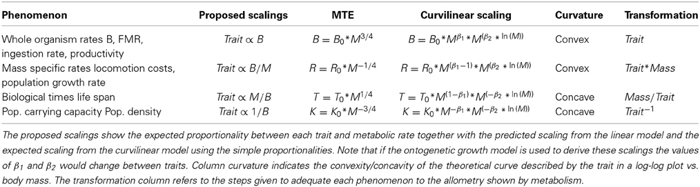
Table 1. Body size and metabolic scaling for different ecological traits/phenomena.

To predict the scaling of developmental times (Gillooly et al., 2002) and rates at the population level (Savage et al., 2004b; Duncan et al., 2007), MTE incorporates Equation 1 in a growth model (West et al., 2001; Hou et al., 2008; Moses et al., 2008) that balances energy uptake and maintenance costs during ontogeny. An important assumption in this general ontogenetic growth model is that the metabolic rate during ontogeny scales with the same allometric coefficient observed across adult animals of different species (Moses et al., 2008; Makarieva et al., 2009; Zuo et al., 2009). So ontogenetic growth is modeled as:

$\begin{array}{ll}\frac{dm}{dt}=a{m}^{\beta }-bm\hfill & (5)\hfill \end{array}$

where m is the mass of the organism as a function of time (t), and a and b are parameters related to fundamental cellular properties (West et al., 2001; Gillooly et al., 2002; Moses et al., 2008).

Integrating Equation 5 from t = birth to t = maturity, yields the prediction that developmental time should scale interspecifically with an exponent equal to β − 1 (Gillooly et al., 2002). MTE then uses demographic theory to make predictions at the population level (i.e., Jetz et al., 2004; Savage et al., 2004b; Duncan et al., 2007; White et al., 2007).

If we follow the same steps, but instead of using Equation 1 we use the curvilinear Equation 4, we obtain the equation:

$\begin{array}{ll}\frac{dm}{dt}=a{m}^{{\beta }_1+{\beta }_2\ln (m)}-bm\hfill & (6)\hfill \end{array}$

whose integral cannot be solved analytically to make predictions on the exact curvilinear scaling of biological times (and hence rates at the population level) with body mass. Intuitively, however, the increasing slope in the allometry of mammalian metabolism should translate to a curvature in the size scaling of other metabolic-mediated traits such as life span, population density or population growth rate. If these curvatures exist they should be perceived as convex for whole organism and mass specific rates, and as concave for biological times and population carrying capacities (Table 1), with critical consequences on species on the extremes of the body size range.

In this work we demonstrate the propagation of the curvature of metabolism through different mammalian life-history traits, both at the individual and population level. We will first show the existence of curvatures in the different life history traits evaluated; then, we will show that the type of curvature in terms of concavity/convexity is different for each trait as expected according to the proportionality between the scaling of each trait and metabolic rate. Because the allometric coefficients change with body size, the existence of such curvilinear relationships prevents any attempts to test MTE on the basis of comparison of linear log-log scaling coefficients unless the ranges of body mass considered by all data sets are the same. Given the low number of species for which all traits have been measured, we will compare the body size scaling of each trait with the size scaling of metabolism for the same subset of species. Finally we will try to solve the differential Equation 6 numerically to understand how the curvature of metabolism should affect the scaling of other biological traits. As explained above, the differential Equation 6 is based on the assumption that interspecific and intraspecific metabolic scalings should be equal, but here we will explore the consequences of the relaxation of this assumption on the curvilinear scaling of metabolic rate.

2. Materials and Methods

2.1. Evaluated Life History Traits

We performed a bibliographic search on life history traits of mammals, both at the organism and at population levels of organization. The result of this compilation is presented Data Sheet 1 in Supplementary Material. Traits at the population level of organization refer to traits varying at the population level for which we are using a species level average. We considered eight different traits (basal metabolic rate in J s⁻¹, field metabolic rate in J s⁻¹, offspring biomass production in kg s⁻¹, ingestion rate in J s⁻¹, costs of locomotion in L O₂ kg⁻¹ m⁻¹, life span in s, population growth rate in s⁻¹ and population density in m⁻²) using nine different bibliographic sources (see Table S1). If available, we obtained the data directly from tables but when tables were not provided we digitized the data from plots (Table S1). The offspring biomass production P was calculated using the clutch size C, the number of clutches produced per year N, and the mass of each individual offspring m, obtaining P = CNm. The data on ingestion rate refers both to carnivores and herbivores from the work of Farlow (1976) (Table S1). Data on body temperatures were compiled from the work of McNab (2008), and are reported also Data Sheet 1 in Supplementary Material.

To homogenize the species names of the different data sets, we followed the nomenclature provided by Fritz et al. (2009). Then, we constructed a database with the values of each trait reported for each mammalian species considered (Data Sheet 1 in Supplementary Material). This compilation results in a total of 1365 species. Data on basal metabolic rate is available for 746 different species combining data from the data-bases of McNab (2008), Sieg et al. (2009), and Savage et al. (2004b). For those species with more than one data reported from the different data sets we calculated an arithmetic mean of the logarithms for B and body mass; these are the values used in the comparisons with the other traits in Figure 3. Data on field metabolic rate is available for 116 species of which 84 have associated values of B. Data on offspring biomass productivity is available for 532 species of which data on B is available for 279 species. In the case of life span, we found values of B for 270 out of 592 species. Data on population growth rate is available for 294 species of which we have values of B in the case of 162 species. Finally, for population density we have values for 553 different species, of which data for B is available for 245 species.

2.2. Influence of Temperature and Phylogeny

Metabolic rate and all the related life history traits are highly influenced by temperature (Ernest et al., 2003; Savage et al., 2004a; White et al., 2006). Although we consider only endotherm mammals, there can be small differences in body temperature between the species. For the analysis of the effect of the temperature in each life history trait, we considered the compilation by McNab (2008), used by Kolokotrones et al. (2010) (see Data Sheet 1 in Supplementary Material). Additionally, in order to account for the non-independence of the data due to the shared evolutionary history of species, we analyzed the different traits by means of phylogenetic least squares regression (PGLS). To do that we used the phylogenetic tree provided by Fritz et al. (2009), which is an updated version of the tree of Bininda-Emonds et al. (2007) considering 5020 species of mammals. The branch lengths and structure of this tree represents the evolutionary history and phylogeny of each species. In consequence, to carry out the PGLS, we first homogenized the species names to the nomenclature used by Fritz et al. (2009) as described above. Once each species has an associated phylogenetic position, we use REstricted Maximum Likelihood (REML) instead of Maximum Likelihood (following the methodology of Kolokotrones et al., 2010) for fitting the models. These analyses were carried out using the APE (Paradis et al., 2004) and NLME (Pinheiro et al., 2014) packages for R (R Core Team, 2014). The parameter λ (Pagel, 1999; Freckleton et al., 2002) of the regressions was also calculated as a measure of the importance of phylogeny on the residuals errors of the regression (Revell, 2010).

2.3. Analysis of the Coincidence of the Curvatures and Measurement Error

To compare the curvilinear fit of B and the curvilinear fits of the other life-history traits, and given that not all the traits follow 3/4 allometries, the values of the traits were transformed so that the expected scaling, based on MTE, would be 3/4. To transform each trait, we followed the mathematical description shown in “Transformation” column of Table 1, which consisted of easy mathematical transformations between B and M. Once the traits were transformed, to test the variation in the linear slopes we performed standard linear regressions of each trait and body size. The 95% confidence intervals of these slopes are shown in Figure S1 with the word “Slope.” The curvatures of the different traits were analyzed by fitting an orthogonal polynomial regression. This regression is of the form Y = α + β(X − X) + γ(X² + aX − b); where X is the average of the X values, and a and b are chosen so that Σ(X² + aX − b) = 0 and ΣX(X² − aX − b) = 0. This method does not affect the estimate of γ and it makes the estimates of α, β and γ independent of each other. Additionally, this method is not affected by changes of scale, so the results are not dependent on the mass unit considered. To compare the coefficients of two orthogonal regressions the average of the X values (i.e., the average body masses) should be equal. For some species the average body mass was different in each trait database, which would make the average body sizes differ. To avoid this error in the calculation of the orthogonal regression coefficients we used an average body mass from the two datasets being compared.

To analyze the effect of measurement error and intraspecific variability in BMR, we performed a similar comparison using BMR estimates reported by two different bibliographic sources for the same species. To create a BMR data set where the measurements for each species come from different sources, we removed from the work of McNab (2008) and Sieg et al. (2009) those species that had the same first author as the original data source (Data Sheet 1 in Supplementary Material). To do that we performed an extensive search on the primary sources used by these studies on BMR. Quite often these sources were citations that compiled data from several sources, although a big effort was done to disentangle these sub-references, it was sometimes impossible to obtain the original data source. For example, although data on mass and BMR for the Chilean rock rat (Aconaemys fuscus) were exactly the same in the two data sets, the data sources (or the sub-references we were able to obtain) were different. We included these species in our data set so our approach is conservative in the sense that some references considered here to be different could come from the same original source. In the case of the BMR data base of Savage et al. (2004b), it was not possible to analyze the bibliographic origin of the data, as the amount of sub-references was too high.

2.4. Analysis of the Influence of the Curvature of Metabolism on the Scaling of Developmental Time

We used a numerical model to test the resulting interspecific scaling of developmental times (and hence traits at the population level) if the assumption of equal ontogenetic and interspecific metabolic scalings is relaxed. As we explained in the introduction, if the curvilinear scaling in B is accepted, the integral of Equation 6 cannot be solved analytically to predict the exact scaling of developmental time and population rates with body size. To solve the differential growth Equation 6 we used the solver for ordinary differential equations, switching automatically between stiff and non-stiff methods (lsoda) (Petzold, 1983) using package “deSolve” in the R statistical package (R Core Team, 2014) (see simulations in Figures 4A,B). The code used to run the simulations presented in Figure 4 is provided in the Presentation 1 in Supplementary Material.

3. Results

3.1. Scaling-Up the Curvature of Metabolism

We have evaluated the propagation of the curvature of metabolic rate through seven different life history traits (see Materials and Methods and Table S1). The log-log plots of these traits vs. body mass show a curvilinear response in most traits (Figure 1, where the traits are ordered from the individual, upper panels, to the population level of organization, lower panels). This visual perception of the curvatures is supported by the better fit and lower Akaike values of the quadratic model compared to the linear fit and the significance of the quadratic term in Equation 3 (Tables 2, 3). Only for population density, where the variability explained by body size is small, the quadratic term is not significant (Table 3). In those cases where the curvature is significant, the convexity and concavity of these curvatures is coincident with the scalings proposed by MTE and shown in Table 1 (sign of β₂ in Table 3).

FIGURE 1

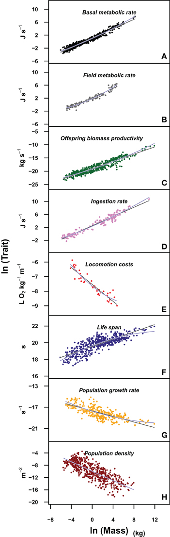
Figure 1. Plots of the different life history traits (A: basal metabolic rate; B: field metabolic rate; C: offspring biomass productivity; D: ingestion rate; E: locomotion costs; F: life span; G: population growth rate; H: population density) vs. body mass in a log-log scale. Blue lines correspond to the fit of the quadratic model and black lines to the fit of a linear model. The upper panels correspond to individual level traits, while the lower panels to population level traits. See Data Sheet 1 in Supplementary Material for the bibliographic sources used to construct each panel.

TABLE 2

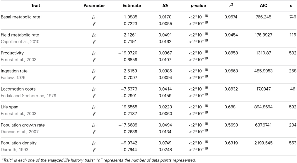
Table 2. Fit of the data in Figure 1 of the main text using a linear (ln(Trait) ~ β₀ + βln(M)) model.

TABLE 3

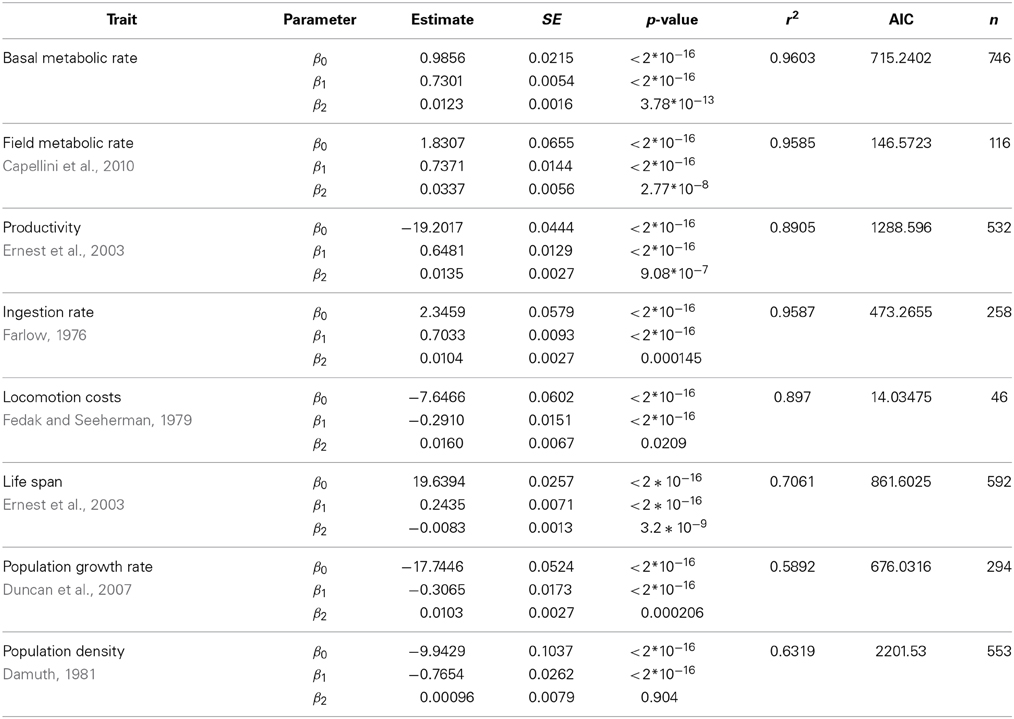
Table 3. Fit of the data in Figure 1 of the main text using a quadratic model (ln(Trait) ~ β₀ + β₁ln(M) + β₂(ln(M))²).

3.2. Influence of Temperature and Phylogeny

When the allometry of these traits was analyzed taking into account the possible effects of body temperature or the phylogenetic relationship of the species within each data set, the curvature remains significant for most traits, except for those traits at the population level (Tables 4, 5). Figure 2 allows a visual comparison of the curvatures of the different traits using the quadratic model with temperature (left panels), and the quadratic model accounting for the phylogenetic history of each species (PGLS regression, right panels). As in Figure 1, the slope and convexity of each relationship depend on the allometric coefficient of the traits. Although the curvatures were statistically significant when temperature and phylogeny are taken into account (Tables 4, 5), the different curvatures obtained among traits may be caused by the lower number of data points and restricted body mass range available when phylogeny, and more critically temperature, are considered (column “n” in Tables 2–5). With some exceptions, the models accounting for phylogeny and temperature have lower Akaike values than the linear or the quadratic fits (Tables 2–5). Besides the high values of λ obtained (Table 5), this means that models considering the phylogeny of species are the most appropriate to evaluate the curvature of the different scaling relationships.

TABLE 4

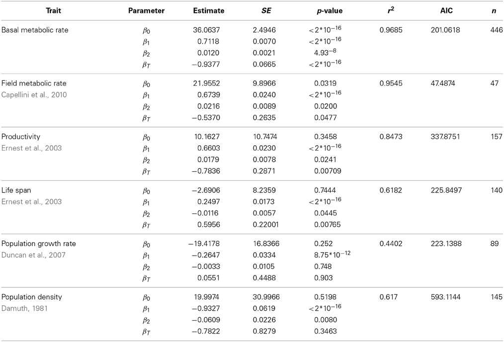
Table 4. Fit of the data shown in left panels of Figure 2, using a quadratic model with a temperature term (ln(Trait) ~ β₀ + β₁ln(M) + β₂(ln(M))² + β_T / T).

TABLE 5

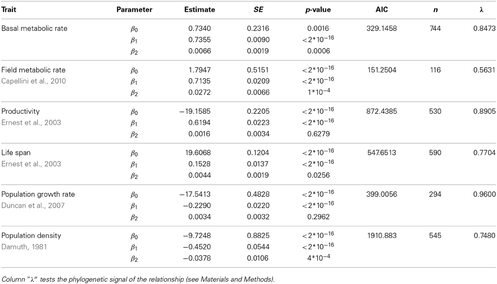
Table 5. Fit of the data shown in right panels of Figure 2 of the main text using phylogenetic least squares regression (ln(Trait) ~ β₀ + β₁ln(M) + β₂(ln(M))²).

FIGURE 2

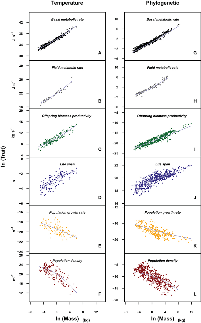
Figure 2. Plots of the different life history traits (A,G: basal metabolic rate; B,H: field metabolic rate; C,I: offspring biomass productivity; D,J: life span; E,K: population growth rate; F,L: population density) vs. body mass in a log-log scale. The models fitted (blue lines) incorporate the effects of temperature (left panels) and phylogeny (right panels). Traits in left panels were corrected for the effect of temperature (ln(Trait/e^(E/kT))). In left panels we fit a quadratic model of the form ln(Trait) β₀ + β₁ * ln(M) + β₂ * ln(M)² + β_T/T, whose coefficient values can be found in Table 4. In right panels, we carry out a phylogenetic least squares regression of the form ln(Trait) β₀ + β₁ * ln(M) + β₂ * ln(M)², whose coefficient values are reported in Table 5.

3.3. Analysis of the Coincidence of Curvatures and Measurement Error

Tests on whether the curvature of each trait is coincident with the curvature found in basal metabolic rate cannot be based on the fits in Figure 1 for two reasons. First, because the estimates of the coefficients for the quadratic term in a traditional least-squares polynomial regression are dependent on the estimates for the linear term, and second, because the body mass ranges in each data set are different (Table S1), thus the expected fits for the linear term should also differ. To resolve these two problems we have performed pairwise comparisons using only those species for which both data on each life history trait and basal metabolic rate were available (Figure S1). We have then used orthogonal polynomial regression to test whether the first and second order polynomial terms coincide (i.e., whether the 95% confidence intervals overlap, see Materials and Methods for details on orthogonal polynomial regression). The confidence intervals for the second term of the polynomial fit overlap in all cases, indicating that the departure from linearity is similar in all cases. However, the estimates for the linear term (i.e., first term of the polynomial) only overlap with those for B in the case of field metabolic rate. For all the other traits analyzed, the allometric scaling coefficients differ, pointing to a mismatch in size scaling between most ecological traits and B.

This novel database with paired estimates of B and life history traits for each species lets us analyze the variance in metabolic rate not explained by body size. If a species has a metabolic rate different from that expected for animals of the same size (a difference measured by the residuals in a plot of metabolism vs body size), this difference should be perceived, following ME, in the residuals of the plots of other traits with body size for that same species. The analysis of the residuals of these body size relationships (Figure 3) indicates that higher residuals in B translate into higher residuals of field metabolic rate, but not into higher residuals for the rest of traits considered. This is an indication that, once the effects of body size on metabolic rate have been accounted for, the remaining variance in metabolic rate does not have any perceptible effects on the other traits.

FIGURE 3

Figure 3. Relationships of the residuals of the linear regression fits of each evaluated trait (A: field metabolic rate; B: offspring biomass productivity; C: life span; D: population growth rate; E: population density) and B. Panel (F) represents the residuals of B from different bibliographic sources (Sieg et al., 2009 in the x-axis and Kolokotrones et al., 2010 in the y-axis).

To fully understand this result, we need to know if the residuals in the metabolism vs. body size relationship are an indication that a given species has a different metabolic rate or it is just the result of random or measurement error. As we pointed out in the introduction, the error term (ϵ) in Equations 2 and 3 includes both the experimental error and the variability not explained by body size. In an attempt to study the magnitude of this experimental error, we have compared two different data sets of basal metabolic rate (the one used by Kolokotrones et al., 2010 to describe the curvature of metabolism McNab, 2008 and the data set of Sieg et al., 2009), considering only those data coming from different bibliographic sources (Figure 3F, but see also Figure S1 panels K, L). The goodness of fit between the residuals of B for each species in the two data sets may be an indication of the relative importance of experimental error and true variability. An analysis of the residuals similar to the one applied above for other traits indicates a correlation between the residuals of both B data sets of 46.2%. In addition, the B estimates of these data sets for each species are the average of several measurements so intraspecific variability is not considered. Sieg et al. (2009) provided data on intraspecific variability measured as the standard deviation of B measurements for different individuals of the same species. For 34% of the species considered in the database used in Figure S1 panel L, the intraspecific variability is larger than the residuals of the B vs. body size plot. Consequently, although the residuals of B vs. body size hold some information, there is quite a lot of scatter introduced by intraspecific variation and measurement error. Body size captures most of the variability in metabolic rate: in this comparison of B measured by different sources, body size explains 95.9% of the variance, while the B measured for the same species by a different author explains 96.7% (Figure S2, panels A, B).

3.4. Analysis of the Influence of the Curvature of Metabolism on the Scaling of Developmental Time

In Figure 4A we provide a numerical example of the prediction of MTE using a simple, linear allometry of B (β₁ = 3/4; β₂ = 0) resulting in the predicted linear scaling of developmental time (γ₁ = 1/4; γ₂ = 0). However, following the same approach using the curvilinear model for B (Table 3) (β₁ = 0.5593; β₂ = 0.0123), the resulting scaling of developmental time has a γ₁ = 0.4746 and a γ₂ = −0.0061 (Figure 4B). Hence, if there is a curvilinear scaling of B with body size, following MTE we reach the counter-intuitive result that the scaling of developmental time should be curvilinear but with different scaling coefficients.

FIGURE 4

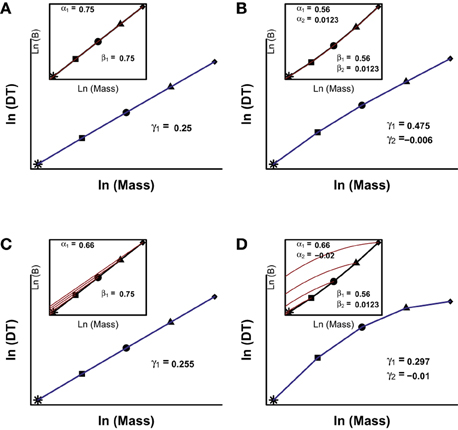
Figure 4. Numerical solutions for Equation 6. The inset in each panel represents the interspecific (black line) and ontogenetic (red lines) scalings of B vs. body size. The different symbols represent hypothetical adult body sizes of different species. The blue lines show the scaling of developmental time (DT, defined as the moment in which the organism reach an arbitrary fraction of adult body size) with body mass. The coefficients shown correspond to the models ln(B_ontogenetic) = a_o + α₁ * ln(m) + α₂ * ln(m)²; ln(B_{interspecific}) = a_i + β₁ * ln(M) + β₂ * ln(M)² and ln(DT) = a₃ + γ₁ * ln(M) + γ₂ * ln(M)²; where m is the mass of the organism during growth and M is the asymptotic adult mass of the species. In (A,B), the ontogenetic and interspecific scalings are coincident; in (C) they are different and linear, and in (D) they are different and curvilinear. See Presentation 1 in Supplementary Material for further details on the mathematical background and the R code to solve the model.

Similarly, Figures 4C,D show two scenarios where the allometry of B during ontogeny is different to the allometry of the interspecific scaling of B. The most simple case is one where both scalings are linear on a log-log scale but ontogenetic B takes an allometric slope lower than interspecific allometric scaling. This reflects the commonly observed phenomenon that a juvenile of a species has a higher mass-specific metabolic rate (B/M) than an adult individual of another species with the same body mass (Makarieva et al., 2009). In Figure 4C, we run a simulation where the slope of ontogenetic scaling is 2/3 and the interspecific scaling 3/4. The result of this simulation is a linear scaling of developmental time with body size, with an interspecific scaling coefficient 0.255. From these simulations we can conclude that the interspecific scaling in B has more importance in the resulting interspecific scaling in developmental time. Figure 4D shows another simulation where ontogenetic and interspecific scalings are different, both are curvilinear and each has a different degree and sign of curvilinearity. In this simulation, the scaling of B is convex between species but concave during ontogeny. The concave curvature of B during ontogeny introduces some degree of variability but the scaling of developmental time is still concave as expected from the interspecific convex scaling of B.

4. Discussion

The curvature of metabolism described by Kolokotrones et al. (2010) seems to be present in the relationship between other important life history traits and body size in mammals. This finding gives support to the fundamental tenet of ME, that metabolism drives the ecology of organisms at any level of biological organization but, given the body size dependence of the expected scaling coefficients, it prevents also to test the validity of MTE based on the comparison of slopes and theoretical scaling coefficients.

The finding that deviations from linear allometries occur is not a novel result. In the physiology and scaling community, certain non-linearity in this relationship has been known for a long time (Peters, 1983; Calder, 1984; Schmidt-Nielsen, 1984; Charnov, 1993; Dodds et al., 2001; Packard and Birchard, 2008; Savage et al., 2008; White et al., 2009; Banavar et al., 2010; Kolokotrones et al., 2010; Ehnes et al., 2011). The work of West et al. (1997), where the constant value of β is demonstrated to be 3/4, considers this and explains how in fractal-like systems of resource distribution, the importance of the term determining the branching of small vessels increases in small animals, what finally causes a slightly different scaling exponent in animals depending on their body size. Similarly, Kolokotrones et al. (2010) have shown that the curvature in metabolic scaling is not against the principles of MTE and that the mechanistic model of West et al. (1999) can be extended to meet the premises of the quadratic equation. Our work is based on the idea that if the principal tenet of ME and the scalings suggested by MTE are correct, (Enquist et al., 2003; Brown et al., 2004; Economo et al., 2005), the curvature of metabolism should be perceived in other ecological traits. In consequence, the fact that most traits considered show a curvature (Figure 1) coincident with the predicted convexity or concavity as expected from MTE, can be considered as a support for ME.

We have found also that when the effect of temperature is considered, the curvature remains significant for the traits at the individual level, but it seems to lose strength when higher order traits are evaluated. Clarke et al. (2010) found that the most appropriate model describing the scaling relationship of basal metabolic rate and body size is a quadratic model including the temperature term. For these authors, the influence of the temperature term is significant, although it has a weak influence on the explanatory power of the model. Additionally, these authors corrected their non-independent data sets by means of phylogenetic analysis and the effect of temperature. By doing so, the importance of the temperature term as a predictive factor for basal metabolic rate decreases even further.

Concerning the persistence of the curvatures when the temperature and the phylogenies are considered in our analysis, Figure 2 and Tables 4, 5 show that, in general, the curvatures remain, albeit they can be less evident in some traits. In any case, the Akaike of the fits considering temperature and phylogeny are, in general, lower than the linear and quadratic fits, indicating that these models are appropriate to evaluate the curvature of scaling. In the case of the phylogenetic approach, the values of λ (Table 5) are reasonably high, which indicates that the phylogenetic influence on these relationships is considerable. This result also indicates the importance of carrying out phylogenetic approaches when performing these kind of comparative analyses. The use of phylogenetic approaches is widely accepted nowadays, and there is no reason to present separate phylogenetic and non-phylogenetic controlled analyses (Freckleton, 2009). The reason why we do so is to allow a better comparison of our results with the curvature of metabolism described by Kolokotrones et al. (2010), where these approaches are also presented separately.

Silva and Downing (1995) have considered the relationship between population density and body size for different groups of mammals. These authors found a negative relationship between population density and body mass, but with a more pronounced slope for smaller animals than for larger organisms. In their study they considered data on population density regardless of whether this was maximal so the energetic equivalence rule (Damuth, 1981) is not expected to hold (Isaac et al., 2011). In addition, the shape of the relationship between population density and body mass remains controversial and some authors argue that it could be triangular instead of linear, with medium sized species attaining a higher density (Marquet et al., 1995). We have chosen to analyze the data set of Damuth (1993) because it considers only the size range for which maximal population density decreases with body size and the energetic equivalence rule should hold.

Charnov and Ernest (2006) studied the allometry of reproductive trade-offs and explored the relationship between the number of offspring produced (corrected for the female mass) and the offspring size. They found a slight curvature or break at a neonate size around 1 kg. Using these data, as well as the number of offspring per clutch and the clutches per year (see Materials and Methods) we obtain the curvature in Figure 1C. The relationship between offspring biomass productivity and body size describes a convex curve that, following MTE, agrees with the concave curvature in B, suggesting that the break found by Charnov and Ernest (2006) could have a metabolic origin. A similar break in the allometric relationships is reported in the work of Brown et al. (1993). Through the development of a theory for optimal body size in mammals based on an energetic point of view, this work is probably the first approach to a non-linear allometric relationship between metabolism and body size, and predicts a break or curvature of different mammalian traits at a mass of 1 kg. This model has been subject to intense debate (e.g., Bokma, 2001) and is nowadays largely discredited, but the skewed frequency distribution of body sizes described might be related to the curvature in metabolism found by Kolokotrones et al. (2010).

Tests on the difference between the allometric scaling of different traits and the scalings predicted by MTE, based on the linear Equation 2, have been used to refute (i.e., Duncan et al., 2007) or accept (i.e., Savage et al., 2004b) MTE. The existence of curvilinear scalings, however, invalidates to some extent all these attempts. The linear (in a log-log scale) coefficients are mass dependent, so a trait would have a scaling coefficient different or similar to 3/4 depending on the body mass range of the database under consideration. Thus, we suggest a way to correctly make these comparisons for each trait by considering a database of B and trait measurements for the same species. Because in such a database the body masses coincide, the linear fits of B and the given trait should be the same if MTE is correct. For the traits considered, such comparisons (Figure S1) lead to the conclusion that the linear fits for all traits (except field metabolic rate) differ.

However, the existence of a curvature in metabolism introduces further uncertainties in the comparison of scaling coefficients. If Equation 3 is accepted as valid, it is not possible to analytically reach the prediction on the expected scalings for developmental time and traits at the population level. Nevertheless Equation 6 can be integrated numerically to show that when the scaling of B is curvilinear, the resulting scaling in developmental time is also curvilinear but with a different degree of curvilinearity (Figure 4). Furthermore, Equation 6 is reached after assuming that during ontogeny the scaling of B with body mass parallels interspecific scaling (Hou et al., 2008; Moses et al., 2008), an assumption which has been the focus of some debate and may not be respected in most of the cases (Glazier, 2005; Makarieva et al., 2009; Zuo et al., 2009). These simulations suggest thus that it is not possible to refute MTE if the scaling coefficients of ecological traits are different to that of B.

A possible way to test ME would be to analyze the residuals of the relationship between B and body size. If a species has a B different than expected for its body size, it should have an influence on its ecology and be reflected in the residuals of other life history traits for this species. However, do the residuals hold ecological information or are they the result of random and experimental noise? Although some phylogenetic groups have been shown to fall above the B vs. mass regression line (McNab, 2008; Capellini et al., 2010), and despite a phylogenetic signal in the linear term of the B scaling exponent has been detected (Capellini et al., 2010; Isaac and Carbone, 2010), these differences are not reflected in the other traits (Figure 3). In any case, it is hard to ascertain to what extent these differences are influenced by common experimental errors due to the use of different protocols to measure B for each group or species, and hence to what extent these deviations should be reflected in the scaling of other traits. For example, one important source of noise in the measurements of B is the number of individuals used to obtain each data point in the data sets (Garamszegi and Møller, 2010; Garamszegi, 2014). We have, however, attempted to assess this experimental error by creating a database where each species has two B measurements each one coming from a different original bibliographic source. If experimental error is very low compared to ecological effects we would expect a good correlation between the two B measurements. The moderate correlation (r² = 0.462, Figure 3F) between the residuals of each B data set indicates that the measurement error of B is considerable. We cannot quantify the magnitude of the measurement error in the values of the other traits considered but it is likely to be, at least, of the same magnitude to that of B. This suggests that, to some extent, the lack of correlation in the plots of Figure 3 could be due to the influence of experimental or random error (White et al., 2012). In addition, intraspecific variability within traits should be considered. Intraspecific variability is larger than the residuals of the B vs body size plot for 34% of the species in our database. Because B and each trait are measured on different sets of individuals this introduces further uncertainty in the comparison of residuals.

In summary, our analysis leaves an uncertain scenario on the acceptance of MTE as a general macroecological theoretical framework. We have shown that testing MTE on the basis of comparison of regression slopes is not a valid approach. Furthermore, the analysis of residuals shows that intraespecific and experimental errors are greater than expected, thus introducing some level of uncertainty in this kind of studies. The pervasive effect of body size on B, explaining a similar amount of variance than B measured in another set of individuals of the same species, makes difficult to analyze the residual variance. Studies measuring B and other ecological traits on the same set of individuals with sample sizes large enough to reduce experimental error are needed to fully evaluate MTE. In any case, the curvatures of the traits, in agreement with the concave/convex scaling expected by ME, point to a regularity in the curvilinear scaling of many different life history traits which could have a metabolic origin.

Conflict of Interest Statement

The authors declare that the research was conducted in the absence of any commercial or financial relationships that could be construed as a potential conflict of interest.

Acknowledgments

This work was partially funded by Theme 6 of the EU Seventh Framework Program through the Marine Ecosystem Evolution in a Changing Environment (MEECE No. 212085), project METOCA funded by Spanish National I+D+I Plan, and project RADIALES from the Instituto Español de Oceanografía. Juan Bueno was a recipient of a PhD fellowship from the Instituto Español de Oceanografía. Authors would like to thank A. Isla, X. A. Morán, T. Huete, F. Cabello, and N. Weidberg for their comments and suggestions on the original paper.

Supplementary Material

The Supplementary Material for this article can be found online at: http://www.frontiersin.org/journal/10.3389/fevo.2014.00061/abstract

References

Banavar, J. R., Moses, M. E., Brown, J. H., Damuth, J., Rinaldo, A., Sibly, R. M., et al. (2010). A general basis for quarter-power scaling in animals. Proc. Natl. Acad. Sci. U.S.A. 107, 15816–15820. doi: 10.1073/pnas.1009974107

Pubmed Abstract | Pubmed Full Text | CrossRef Full Text | Google Scholar

Bininda-Emonds, O. R. P., Cardillo, M., Jones, K. E., MacPhee, R. D. E., Beck, R. M. D., Grenyer, R., et al. (2007). The delayed rise of present-day mammals. Nature 446, 507–512. doi: 10.1038/nature05634

Pubmed Abstract | Pubmed Full Text | CrossRef Full Text | Google Scholar

Bokma, F. (2001). Evolution of body size: limitations of an energetic definition of fitness. Funct. Ecol. 15, 696–699. doi: 10.1046/j.0269-8463.2001.00548.x

CrossRef Full Text | Google Scholar

Brown, J. H., Gillooly, J. F., Allen, A. P., Savage, V. M., and West, G. B. (2004). Toward a metabolic theory of ecology. Ecology 85, 1771–1789. doi: 10.1890/03-9000

CrossRef Full Text | Google Scholar

Brown, J. H., Marquet, P. A., and Taper, M. L. (1993). Evolution of body size: consequences of an energetic definition of fitness. Am. Nat. 142, 573–584. doi: 10.1086/285558

Pubmed Abstract | Pubmed Full Text | CrossRef Full Text | Google Scholar

Brown, J. H., and Sibly, R. M. (2012). “The metabolic theory of ecology and its central equation,” in Metabolic Ecology: a Scaling Approach, eds R. M. Sibly, J. H. Brown, and A. Kodric-Brown (Chichester, UK: John Wiley & Sons, Ltd.). doi: 10.1002/9781119968535.ch2

CrossRef Full Text | Google Scholar

Brown, J. H., Sibly, R. M., and Kodric-Brown, A. (2012). “Metabolism as the basis for a theoretical unification of ecology,” in Metabolic Ecology: a Scaling Approach, eds R. M. Sibly, J. H. Brown and A. Kodric-Brown (Chichester, UK: John Wiley & Sons, Ltd.). doi: 10.1002/9781119968535.ch

CrossRef Full Text | Google Scholar

Calder, W. A. (1984). Function and Life History. Cambridge, MA: Harvard University Press.

Google Scholar

Capellini, I., Venditi, C., and Barton, R. A. (2010). Phylogeny and metabolic scaling in mammals. Ecology 91, 2783–2793. doi: 10.1890/09-0817.1

Pubmed Abstract | Pubmed Full Text | CrossRef Full Text | Google Scholar

Charnov, E. L. (1993). Life History Invariants. Oxford: Oxford University Press.

Charnov, E. L., and Ernest, S. K. M. (2006). The offspring-size/clutch-size trade-off in mammals. Am. Nat. 167, 578–582. doi: 10.1086/501141

Pubmed Abstract | Pubmed Full Text | CrossRef Full Text | Google Scholar

Clarke, A., Rothery, P., and Isaac, N. J. B. (2010). Scaling of basal metabolic rate with body mass and temperature in mammals. J. Anim. Ecol. 79, 610–619. doi: 10.1111/j.1365-2656.2010.01672.x

Pubmed Abstract | Pubmed Full Text | CrossRef Full Text | Google Scholar

Damuth, J. (1981). Population density and body size in mammals. Nature 290, 699–700. doi: 10.1038/290699a0

CrossRef Full Text | Google Scholar

Damuth, J. (1993). Cope's rule, the island rule and the scaling of mammalian population density. Nature 365, 748–750. doi: 10.1038/365748a0

Pubmed Abstract | Pubmed Full Text | CrossRef Full Text | Google Scholar

Deeds, E. J., Savage, V., and Fontana, W. (2011). Curvature in metabolic scaling: a reply to mackay. J. Theor. Biol. 280, 197–198. doi: 10.1016/j.jtbi.2011.03.036

Pubmed Abstract | Pubmed Full Text | CrossRef Full Text

Dodds, P. S., Rothman, D. H., and Weitz, J. S. (2001). Re-examination of the “3/4-law” of metabolism. J. Theor. Biol. 209, 9–27. doi: 10.1006/jtbi.2000.2238

Pubmed Abstract | Pubmed Full Text | CrossRef Full Text | Google Scholar

Duncan, R. P., Forsyth, D. M., and Hone, J. (2007). Testing the metabolic theory of ecology: allometric scaling exponents in mammals. Ecology 88, 324–333. doi: 10.1890/0012-9658(2007)88[324:TTMTOE]2.0.CO;2

Pubmed Abstract | Pubmed Full Text | CrossRef Full Text | Google Scholar

Economo, E. P., Kerkhoff, A. J., and Enquist, B. J. (2005). Allometric growth, life-history invariants and population energetics. Ecol. Lett. 8, 353–360. doi: 10.1111/j.1461-0248.2005.00737.x

CrossRef Full Text | Google Scholar

Ehnes, R. B., Rall, B. C., and Brose, U. (2011). Phylogenetic grouping, curvature and metabolic scaling in terrestrial invertebrates. Ecol. Lett. 14, 993–1000. doi: 10.1111/j.1461-0248.2011.01660.x

Pubmed Abstract | Pubmed Full Text | CrossRef Full Text | Google Scholar

Enquist, B. J., Economo, E. P., Huxman, T. E., Allen, A. P., Ignace, D. D., and Gillooly, J. F. (2003). Scaling metabolism from organisms to ecosystems. Nature 423, 639–642. doi: 10.1038/nature01671

Pubmed Abstract | Pubmed Full Text | CrossRef Full Text | Google Scholar

Ernest, S. K. M. (2003). Life history characteristics of placental non-volant mammals. Ecology 84:3401. doi: 10.1890/02-9002

CrossRef Full Text | Google Scholar

Ernest, S. K. M., Enquist, B. J., Brown, J. H., Charnov, E. L., Gillooly, J. F., Savage, V., et al. (2003). Thermodynamic and metabolic effects on the scaling of production and population energy use. Ecol. Lett. 6, 990–995. doi: 10.1046/j.1461-0248.2003.00526.x

CrossRef Full Text | Google Scholar

Farlow, J. O. (1976). A consideration on the trophic dynamics of a late cretaceous large-dinosaur community (Oldman formation). Ecology 57, 841–857. doi: 10.2307/1941052

CrossRef Full Text | Google Scholar

Fedak, M. A., and Seeherman, H. J. (1979). Reappraisal of energetics of locomotion show identical cost in bipeds and quadrupeds including ostrich and horse. Nature 282, 713–716. doi: 10.1038/282713a0

Pubmed Abstract | Pubmed Full Text | CrossRef Full Text | Google Scholar

Freckleton, P. (2009). The seven deadly sins of comparative analysis. J. Evol. Biol. 22, 1367–1375. doi: 10.1111/j.1420-9101.2009.01757.x

Pubmed Abstract | Pubmed Full Text | CrossRef Full Text | Google Scholar

Freckleton, P., Harvey, P. H., and Pagel, M. (2002). Phylogenetic analysis and comparative data: a test and review of evidence. Am. Nat. 160, 712–726. doi: 10.1086/343873

Pubmed Abstract | Pubmed Full Text | CrossRef Full Text | Google Scholar

Fritz, S. A., Bininda-Emonds, O. R. P., and Purvis, A. (2009). Geographical variation in predictors of mammalian extinction risk: big is bad, but only in the tropics. Ecol. Lett. 12, 538–549. doi: 10.1111/j.1461-0248.2009.01307.x

Pubmed Abstract | Pubmed Full Text | CrossRef Full Text | Google Scholar

Garamszegi, L. Z. (ed.). (2014). “Uncertainties due to within-species variation in comparative studies: measurement errors and statistical weights,” in Modern Phylogenetic Comparative Methods and Their Application in Evolutionary Biology (Berlin: Springer-Verlag), 157–199. doi: 10.1007/978-3-662-43550-2_7

CrossRef Full Text | Google Scholar

Garamszegi, L. Z., and Møller, A. P. (2010). Effects of sample size and intraspecific variation in phylogenetic comparative studies: a meta-analytic review. Biol. Rev. 85, 797–805. doi: 10.1111/j.1469-185X.2010.00126.x

Pubmed Abstract | Pubmed Full Text | CrossRef Full Text | Google Scholar

Gillooly, J. F., Charnov, E. L., West, G. B., Savage, V. M., and Brown, J. H. (2002). Effects of size and temperature on developmental time. Nature 417, 70–73. doi: 10.1038/417070a

Pubmed Abstract | Pubmed Full Text | CrossRef Full Text | Google Scholar

Glazier, D. S. (2005). Beyond the “3/4-power law”: variation in the intra-and interspecific scaling of metabolic rate in animals. Biol. Rev. 80, 611–662. doi: 10.1017/S1464793105006834

Pubmed Abstract | Pubmed Full Text | CrossRef Full Text | Google Scholar

Glazier, D. S. (2014). Is metabolic rate a universal pacemaker for biological processes? Biol. Rev. Camb. Philos. Soc. doi: 10.1111/brv.12115. [Epub ahead of print].

Pubmed Abstract | Pubmed Full Text | CrossRef Full Text | Google Scholar

Hayssen, V., and Lacy, R. C. (1985). Basal metabolic rates in mammals: taxonomic differences in the allometry of BMR and body mass. Comp. Biochem. Physiol. A 81, 741–754.

Pubmed Abstract | Pubmed Full Text | Google Scholar

Heusner, A. (1982). Energy metabolism and body size. I. is the 0.75 mass exponent of Kleiber a statistical artifact? Respir. Physiol. 48, 1–12. doi: 10.1016/0034-5687(82)90046-9

Pubmed Abstract | Pubmed Full Text | CrossRef Full Text | Google Scholar

Hou, C., Zuo, W., Moses, M. E., Woodruff, W. H., Brown, J. H., and West, G. B. (2008). Energy uptake and allocation during ontogeny. Science 322, 736–739. doi: 10.1126/science.1162302

Pubmed Abstract | Pubmed Full Text | CrossRef Full Text | Google Scholar

Isaac, N. J. B., and Carbone, C. (2010). Why are metabolic scaling exponents so controversial? quantifying variance and testing hypotheses. Ecol. Lett. 13, 728–738. doi: 10.1111/j.1461-0248.2010.01461.x

Pubmed Abstract | Pubmed Full Text | CrossRef Full Text | Google Scholar

Isaac, N. J. B., Storch, D., and Carbone, C. (2011). Taxonomic variation in size density relationships challenges the notion of energy equivalence. Biol. Lett. 7, 615–618. doi: 10.1098/rsbl.2011.0128

Pubmed Abstract | Pubmed Full Text | CrossRef Full Text | Google Scholar

Jetz, W., Carbone, C., Fulford, J., and Brown, J. H. (2004). The scaling of animal space use. Science 306, 266–268. doi: 10.1126/science.1102138

Pubmed Abstract | Pubmed Full Text | CrossRef Full Text | Google Scholar

Kolokotrones, T., Savage, V., Deeds, E. J., and Fontana, W. (2010). Curvature in metabolic scaling. Nature 464, 753–756. doi: 10.1038/nature08920

Pubmed Abstract | Pubmed Full Text | CrossRef Full Text | Google Scholar

Mackay, N. J. (2011). Mass scale and curvature in metabolic scaling. comment on: T. Kolokotrones et al., Curvature in metabolic scaling, Nature 464 (2010) 753-756. J. Theor. Biol. 280, 194–196. doi: 10.1016/j.jtbi.2011.02.011

Pubmed Abstract | Pubmed Full Text | CrossRef Full Text

Makarieva, A. M., Gorshkov, V. G., and Li, B. L. (2009). Comment on “energy uptake and allocation during ontogeny.” Science 325:1206. doi: 10.1126/science.1171303

CrossRef Full Text | Google Scholar

Marquet, P. A., Navarrete, S. A., and Castilla, J. C. (1995). Body size, population density, and the energetic equivalence rule. J. Anim. Ecol. 64, 325–332. doi: 10.2307/5894

CrossRef Full Text | Google Scholar

McNab, B. K. (2008). An analysis of the factors that influence the level and scaling of mammalian BMR. Comp. Biochem. Physiol. A 151, 5–28. doi: 10.1016/j.cbpa.2008.05.008

Pubmed Abstract | Pubmed Full Text | CrossRef Full Text | Google Scholar

Moses, M. E., Hou, C., Woodruff, W. H., West, G. B., Nekola, J. C., Zuo, W., et al. (2008). Revisiting a model of ontogenetic growth: estimating model parameters from theory and data. Am. Nat. 171, 632–645. doi: 10.1086/587073

Pubmed Abstract | Pubmed Full Text | CrossRef Full Text | Google Scholar

Packard, G. C., and Birchard, G. F. (2008). Traditional allometric analysis fails to provide a valid predictive model for mammalian metabolic rates. J. Exp. Biol. 211, 3581–3587. doi: 10.1242/jeb.023317

Pubmed Abstract | Pubmed Full Text | CrossRef Full Text | Google Scholar

Pagel, M. (1999). Inferring the historical patterns of biological evolution. Nature 401, 877–884. doi: 10.1038/44766

Pubmed Abstract | Pubmed Full Text | CrossRef Full Text | Google Scholar

Paradis, E., Claude, J., and Strimmer, K. (2004). Ape: analyses of phylogenetics and evolution in R language. Bioinformatics 20, 289–290. doi: 10.1093/bioinformatics/btg412

Pubmed Abstract | Pubmed Full Text | CrossRef Full Text | Google Scholar

Peters, R. H. (1983). The Ecological Implications of Body Size. Cambridge: Cambridge University Press. doi: 10.1017/CBO9780511608551

CrossRef Full Text | Google Scholar

Petzold, L. R. (1983). Automatic selection of methods for solving stiff and nonstiff systems of ordinary differential equations. SIAM J. Sci. Comput. 4, 136–148. doi: 10.1137/0904010

CrossRef Full Text | Google Scholar

Pinheiro, J., Bates, D., DebRoy, S., Sarkar, D., and R Core Team (2014). nlme: Linear and Nonlinear Mixed Effects Models. R package version 3.1-117.

R Core Team. (2014). R: A Language and Environment for Statistical Computing. Vienna: R Foundation for Statistical Computing. Available online at: http://www.r-project.org

Revell, L. J. (2010). Phylogenetic signal and linear regression on species data. Methods Ecol. Evol. 1, 319–329. doi: 10.1111/j.2041-210X.2010.00044.x

CrossRef Full Text | Google Scholar

Savage, V., Deeds, E. J., and Fontana, W. (2008). Sizing up allometric scaling theory. PLoS Comput. Biol. 4:e1000171. doi: 10.1371/journal.pcbi.1000171

Pubmed Abstract | Pubmed Full Text | CrossRef Full Text | Google Scholar

Savage, V. M., Gillooly, J. F., Brown, J. H., West, G. B., and Charnov, E. L. (2004a). Effects of body size and temperature on population growth. Am. Nat. 163, 429–441. doi: 10.1086/381872

Pubmed Abstract | Pubmed Full Text | CrossRef Full Text | Google Scholar

Savage, V. M., Gillooly, J. F., Woodruff, W. H., West, G. B., Allen, A. P., Enquist, B. J., et al. (2004b). The predominance of quarter-power scaling in biology. Funct. Ecol. 18, 257–282. doi: 10.1111/j.0269-8463.2004.00856.x

CrossRef Full Text | Google Scholar

Schmidt-Nielsen, K. (1984). Scaling: Why is Animal Size so Important? Cambridge: Cambridge University Press. doi: 10.1017/CBO9781139167826

CrossRef Full Text | Google Scholar

Sieg, A. E., O'Connor, M. P., McNair, J. N., and Grant, B. W. (2009). Mammalian metabolic allometry: do intraspecific variation, phylogeny and regression model matters? Am. Nat. 174, 720–733. doi: 10.1086/606023

Pubmed Abstract | Pubmed Full Text | CrossRef Full Text | Google Scholar

Silva, M., and Downing, J. A. (1995). The allometric scaling of density and body mass: a nonlinear relationship for terrestrial mammals. Am. Nat. 145, 704–727. doi: 10.1086/285764

CrossRef Full Text | Google Scholar

West, G. B., Brown, J. H., and Enquist, B. J. (1997). A general model for the origin of allometric scaling laws in biology. Science 276, 122–126. doi: 10.1126/science.276.5309.122

Pubmed Abstract | Pubmed Full Text | CrossRef Full Text | Google Scholar

West, G. B., Brown, J. H., and Enquist, B. J. (1999). The fourth dimension of life: fractal geometry and allometric scaling of organisms. Science 284, 1677–1679. doi: 10.1126/science.284.5420.1677

Pubmed Abstract | Pubmed Full Text | CrossRef Full Text | Google Scholar

West, G. B., Brown, J. H., and Enquist, B. J. (2001). A general model for ontogenetic growth. Nature 413, 628–631. doi: 10.1038/35098076

Pubmed Abstract | Pubmed Full Text | CrossRef Full Text | Google Scholar

White, C., and Kearney, M. R. (2013). Determinants of inter-specific variation in basal metabolic rate. J. Comp. Physiol. B 183, 1–26. doi: 10.1007/s00360-012-0676-5

Pubmed Abstract | Pubmed Full Text | CrossRef Full Text | Google Scholar

White, C. R., Blackburn, T. M., and Seymour, R. S. (2009). Phylogenetically informed analysis of the allometry of mammalian basal metabolic rate supports neither geometric nor quarter-power scaling. Evolution 63, 2658–2667. doi: 10.1111/j.1558-5646.2009.00747.x

Pubmed Abstract | Pubmed Full Text | CrossRef Full Text | Google Scholar

White, C. R., Phillips, N. F., and Seymour, R. S. (2006). The scaling and temperature dependence of vertebrate metabolism. Biol. Lett. 2, 125–127. doi: 10.1098/rsbl.2005.0378

Pubmed Abstract | Pubmed Full Text | CrossRef Full Text | Google Scholar

White, C. R., and Kearney, M. R. (2014). Metabolic scaling in animals: methods, empirical results, and theoretical explanations. Compr. Physiol. 4, 231–256. doi: 10.1002/cphy.c110049

Pubmed Abstract | Pubmed Full Text | CrossRef Full Text | Google Scholar

White, C. R., Schimpf, N. G., and Cassey, P. (2012). The repeatability of metabolic rate declines with time. J. Exp. Biol. 216, 1763–1765. doi: 10.1242/jeb.076562

Pubmed Abstract | Pubmed Full Text | CrossRef Full Text | Google Scholar

White, C. R., and Seymour, R. S. (2003). Mammalian basal metabolic rate is proportional to body mass ^2/3. Proc. Natl. Acad. Sci. U.S.A. 100, 4046–4049. doi: 10.1073/pnas.0436428100

Pubmed Abstract | Pubmed Full Text | CrossRef Full Text | Google Scholar

White, E. P., Ernest, S. K. M., Kerkhoff, A. J., and Enquist, B. J. (2007). Relationships between body size and abundance in ecology. Trends Ecol. Evol. 22, 323–330. doi: 10.1016/j.tree.2007.03.007

Pubmed Abstract | Pubmed Full Text | CrossRef Full Text | Google Scholar

Zuo, W., Moses, M. E., Hou, C., Woodruff, W. H., West, G. B., and Brown, J. H. (2009). Response to comments on energy uptake and allocation during ontogeny. Science 325:1206. doi: 10.1126/science.1171949

CrossRef Full Text | Google Scholar