Environmental Gradients and Spatial Patterns of Calanoid Copepods in the Southeast Pacific

Understanding the mechanisms maintaining the biodiversity of plankton communities in marine ecosystems subject to a strongly variable ocean has become a critical issue for modern oceanography. Here, we used data on distribution of calanoid copepods in the upper layer of the ocean (0–500 m), a widely distributed taxonomic group in the pelagic realm, to assess the effects of changing oceanographic conditions on their diversity patterns and family and species richness. Copepods abundance and occurrence were evaluated from 2002 to 2015 covering the region extended between the coastal upwelling zone (CUP-Z) and the offshore region of Chile at subtropical and temperate areas. We used spatial analyses of community structure descriptors, such as abundance and diversity (family and species richness), multivariate analysis and General Additive Models (GAM_S) in order to study the effect of surface temperature and its gradients, mixed layer depth, salinity and Chlorophyll-a on copepod diversity. Seventeen families were identified comprising 151 species distributed in 3 predefined zones in the onshore-offshore gradient covering the coastal upwelling, the coastal transition and the oligotrophic zones, whereas over the alongshore gradient, same families were majorly linked to the northern and southern portions of the sampled area (20–40°S). Families and species were significantly structured over the zonal gradient, revealing the dominant habitat for each of the families. Spatial patterns revealed the presence of transitional zones comprised by mixed taxa. Over the alongshore gradient this transition zone was linked to the subtropical convergence (30°S). The spatial variation of sea surface temperature (SST) revealed strong environmental zonation of temperature gradients across onshore-offshore and alongshore dimensions. Mean SST combined with mean mixed layer depth explained about 40% and about 29% of variation in family and species richness, respectively over the onshore-offshore axis. We thus conclude that the environmental zonation imposed by SST and its spatial gradients, considered as ecological barriers, is the key driver for maintaining diversity of copepods in the southeast Pacific.

Introduction

The marine pelagic environment presents a high diversity of organisms as part of a complex trophic food web (Lenz, 2012). One of the main groups within the pelagic community is the zooplankton, mostly comprised by species with short life cycles (<1 year), and which is considered a key trophic link in the marine food web and. Zooplankton exhibit a high taxonomic diversity highly sensitive to environmental changes (Peijnenburg and Goetze, 2013; Pino-Pinuer et al., 2014), in particular their changes in abundance and distribution can be used as indicators of ecosystem response to climate driven variation (Beaugrand, 2003; Richardson, 2008).

Actually, the knowledge and understanding of oceanographic drivers influencing patterns of the large-scale distribution of zooplankton over large-scale domains, such as ocean basins is poor, limiting our capacity to predict changes in diversity and spatial distribution under a changing ocean. Biodiversity and species distribution of zooplankton are known to be affected by changes in oceanographic conditions, such as temperature, oxygenation, salinity and stratification, as it has been demonstrated in other regions of the world (Beaugrand et al., 2002; Beaugrand, 2003; Richardson and Schoeman, 2004; Peterson et al., 2006; Aronés et al., 2009; Gewin, 2010; Seibel, 2011), revealing the strong dependence of these organisms on oceanographic variables due to their limited migration capacity and so reflecting the strong effects of hydrographic patterns on their distribution and that of their prey (McClain and Barry, 2010). In this context, the Southeast Pacific (SEP) shows a great heterogeneity in hydrographic conditions from coastal to open sea gradient evidenced by a progressive increase of depth of the mixing layer, dissolved oxygen, temperature and surface salinity (Palma and Silva, 2006; González et al., 2019). Also, within the same gradient it is possible to observe drastic changes in biological productivity, which is high in the coastal zone (Humboldt Current) and extremely low in the ultra-oligotrophic central gyre (Bonnet et al., 2008; Morel et al., 2010; Kletou and Hall-Spencer, 2012; Mann and Lazier, 2013). Across the alongshore gradient (72–110°S), strong differences in temperature, salinity and levels of oxygenation of surface waters can occur. These changes are also accompanied by variable seasonal regimes from low to high latitudes (Strub et al., 1998).

The strong hydrographic variability observed in the SEP over both zonal and meridional gradients allows us to distinguish distinct ecoregions, where the environmental characteristics are seasonal, although relatively stable and homogeneous with respect to the adjacent ones, and such properties are also reflected in distinct communities between these ecoregions. For instance, along coastal and oceanic areas of the SEP five ecoregions have been suggested: Central Peru, Humboldtian, Central Chile, Araucanian, Juan Fernandez, and Desventuradas (Spalding et al., 2007). Although, a recent work based on ecological and biogeochemical division of zooplankton, proposed the existence of four regions over the zonal gradient, predefined in terms of surface chlorophyll-a as a proxy for productivity (González et al., 2019). Same work suggested that changes in the community structure of zooplankton in the SEP could be linked to the factors or processes that modulate the availability of nutrients at lower trophic levels, such as N-limitation and N-fixation (González et al., 2019). Nevertheless, it has now become clear that a changing temperature of the ocean is the major driver for altered diversity and distribution patterns of marine organisms (Antão et al., 2020).

Changes in temperature and sea level have modified the geographical range of some copepod species (Gee, 1991; Crame, 1993; Molfino, 1994), also affecting their evolutionary history (Cronin and Schneider, 1990; Beaugrand et al., 2002). On a smaller scale, ecological factors influencing the physiology of the species can modify the spatial and temporal distribution of species, depending on their tolerance and optimal ranges of their populations, regulating diversity patterns. Such spatial and temporal variation, from microscale to large scale, has contributed synergistically to promote speciation events, and hence shaping up the actual patterns of biodiversity of pelagic organisms. However, the mechanisms that regulate biogeographical patterns need a better understanding to gain tools for predicting the variation in the species distribution under the effect of natural or anthropogenic impacts. Under this view, the pelagic ecosystem of the Southeast Pacific may constitute a suitable model to enhance our understanding of underlying mechanisms modulating zooplankton distribution patterns and other higher trophic levels. With these ultimate goals in mind, in this work we assessed the coastal-oceanic (zonal) and alongshore (meridional) distribution of pelagic Calanoid families and their species over pre-defined zones to test the hypothesis that ecological zonation is determined by environmental gradients of which the temperature gradient can play a unique role. We thus aimed at understanding the underlying mechanisms influencing the large-scale patterns of species distribution within ocean basins.

Materials and Methods

Study Area and Data Bases

The Southeast Pacific region off Chile has been the focus of various zooplankton studies and samplings over the last two decades carried out for our research team, although most of them in the coastal zone, also known as the southern portion of the Humboldt Current system covering the area between 18°S and 40°S. We have also conducted a few oceanographic cruises in the offshore region, even reaching the area near Easter Island (∼110° W). Figure 1 illustrates our study area and the sites from which zooplankton samples have been obtained and used in this study and information of the samples sources and data are summarized in Supplementary Table S1. González et al. (2019) distinguished four ecological zones in this region, as based on the surface chlorophyll-a (Chla-a) concentration, from the highly productive upwelling area toward the central south Pacific gyre. This study found significant changes in zooplankton community structure among these zones, defined as: the CUP-Z, the coastal transition zone (CTZ), the oligotrophic zone (OLIGO-Z) and the ultra-oligotrophic zone (U-OLIGO-Z) which are illustrated in Figure 1. Here, we used these pre-defined zones to allocate all the sampling sites, although the OLIGO-Z and the U-OLIGO-Z were considered only as OLIGO-Z, because of too few samples to separate them.

FIGURE 1

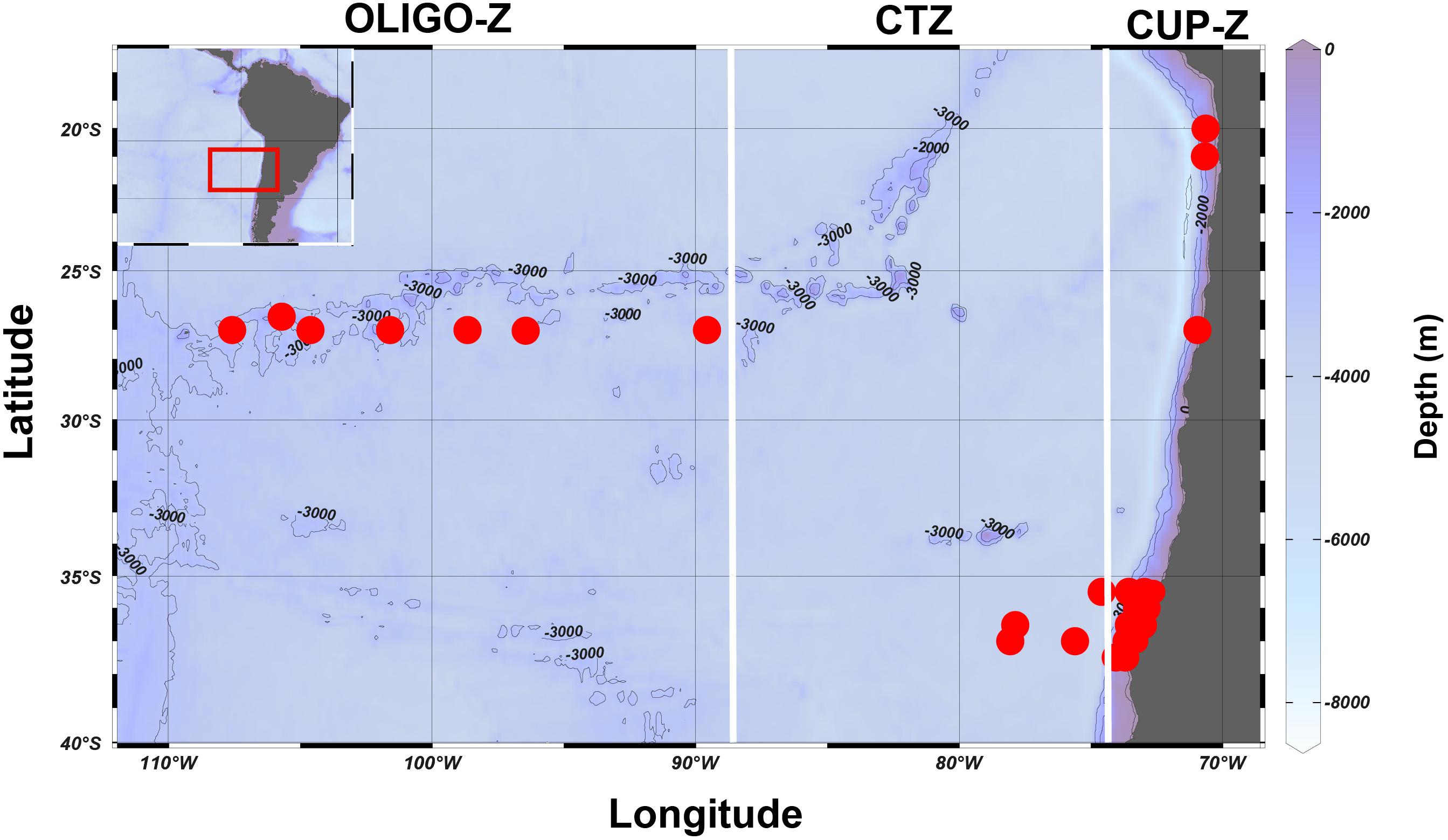
Figure 1. The southeast Pacific region where the samplings were made between the years 2002–2015. The sampling stations are indicated by a red circle. The study area was divided in three zones according to surface chlorophyll-a values: coastal upwelling zone (CUP-Z), mesotrophic coastal transition zone (CTZ), and oligotrophic zone (OLIGO-Z) (González et al., 2019). The bathymetry of each zone is indicated by its color and isobars.

The sampling period for our study was extended from 2002 to 2015 with seasonal variable periods and with different sampling gears (see Supplementary Table S1), although in all cases the target community has been mesozooplankton (200–2000 μm) which is the zooplankton majorly composed by copepods in the ocean. Although most samples have been performed in the upper 200 m, some of them were obtained down to 500 m over OLIGO-Z zone. In the coastal zone a site is part of a coastal time series, so that it has a much better temporal resolution upon monthly sampling, in comparison with all the others for which in some cases a single sampling was done. Most of these data have been published as indicated in Supplementary Table S1 and the copepod data base has been uploaded in the South Pacific node of the Ocean Biogeographic Information Systems (OBIS)¹.

Data Analyses

Data on species abundance from all sampling sites were used as number of individual m^–3. Species have been properly identified and only a few uncertain species are considered at the genera level. For each sampling point the sum of abundance for all species and families was made. However, since the source of samples varied with season, depth strata and sampling gear, the effects of such factors on species abundances and composition were tested with variance analysis (ANOVA), firstly tested for normality and variance homogeneity by Shapiro–Wilks and Levene tests, respectively (see Supplementary Table S2). ANOVA test showed no seasonal or sampling gear effects, but significant differences between depth strata were found, so that data and analyses were treated separately into shallow (0–200 m) and deep (0–500 m) strata.

Changes in copepod families were evaluated for the different zones using community descriptors, such as family richness (R) which is the number of species per family, numerical abundance (N) and weighed frequency of occurrence (WFO) defined as:

$$WFO=\left(\frac{\frac{NFi}{NS}}{REFi}\right).$$

where NF is the number of stations in which the I family was present, NS is total number of sampled stations and REF is the number of species present in the I family. Also, we modified the equation of weighted mean depth suggested by Andersen et al. (2004), as to estimate the average weighted family abundance found across the meridional and zonal gradients of the SEP. For this, we estimated the weighted abundance across the zonal (ZWA) and meridional (MWA) gradients of the copepod families as:

$$ZWAorMWA=\frac{\sum (NiZiRi)}{\sum (NiRi)}.$$

where Ni is standardized sum abundance to ind.m^–3 for family i, Zi is the distance in km between a predefined starting point and end point of a given study area i and Ri is half the difference between these predefined boundaries of their i zone.

Satellite data as on sea surface temperature (SST), mixed layer depth (MLD), sea surface salinity (SSS) and surface Chl-a were used as independent variables during the study period (August 2002 until October 2015). Mean values of these variables were calculated for each sampling station from monthly satellite data. Also, the spatial gradients of SST, both zonal and alongshore were estimated for these mean values for the entire study area. These spatial gradients represent the either alongshore (meridional) or onshore-offshore (zonal) difference in temperature between two consecutive SST means at 1 degree (110 km) spatial resolution. MLD and SSS were obtained from the ARGO floats² with a spatial resolution of 3 degrees, while surface Chl-a was downloaded from the MODIS satellite³ with a spatial resolution of 0.8 degrees. SST was obtained from OAFlux project⁴ with a spatial resolution of 1 degree.

Statistical Analysis

We assessed similarities in distribution of Calanoid copepods families and species only for the shallow stratum (0–200 m), within and between zones, in terms of abundance (individuals m^–3) across a zonal transect. This zonal gradient could not be assessed for the deep stratum (0–500 m), because most samples were only within oceanic region. The analysis of the alongshore distribution of families and species was also restricted to north-south comparisons with respect to the subtropical convergence (ca. 30°S), because of low coverage of the whole gradient and unbalanced design, due to a large number of samples for the southern area 36°S and few of them in the northern portion of the SEP. The structure of the community was evaluated by multivariate analysis performed with PRIMER v.7 (Anderson, 2008). For this, we grouped the different samples over the zonal gradient in according to their location, as CUP-Z, CTZ, and OLIGO-Z. For evaluating similarity in composition and abundance between and within zones, we applied a multidimensional scaling (MDS) and analysis of similarities (ANOSIM) with log-transformed data [Log (x + 1)] for families and presence/absence for species. We used presence and absence data for species, because in some cases only genera were reported, also to reduce extremely high variance of abundances due to presence of dominant and rare species. The matrices of similarities were built for families from the Bray–Curtis index and for species with Jaccard distance. The differences or similarities between the zones were evaluated with SIMPER (percentages of similarity). Also, R Statistic analysis was applied to test differences between groups.

Biota-environmental (BIOENV), Distance-based Linear Model (DISTLM), and Generalized Additive Models (GAM_s) were used to correlate the copepod community with environmental. For this, the abundance of species and families were used as response variables for DISTLM, while for GAM_s and BIOENV richness values were used as dependent variable in order to determine variables to be included in the models, a correlation analysis using Spearman’s test and variance inflation factor (VIF), among the hydrographic variables was first carried out. SSS was found to have strong correlations (r > 0.60 and VIF > 5) with SST, Chl-a and MLD, and it was therefore removed from the analysis in order to minimize collinearity among independent variables. In the BIOENV analysis, similarity matrices were built between log-normalized environmental variables and both family and species richness using Euclidean distance, delivering as result the Sperman rank correlation between the two variables. An automated, stepwise procedure were used both DISTLM and GAM_S analyzes to identify influential variables on families and species richness, and the final model for each diversity measure were obtained according to the Akaike information criterion (AIC). Smaller values of the AIC indicate a better model and yield into the “best” combination of environmental predictor variables that explain the largest amount of variation in the response variable. For DISTLM analysis, similarity matrices were built between the abundance of species and families with the log-normalized environmental variables using Bray-Curtis distance, delivering as result a “Pseudo-F statistic” for each environmental variable. Both the BIOENV and DISTLM analyzes were performed with PRIMER v.7 (Anderson, 2008). Finally, for the GAM_S analysis percent deviance explained (DE) and determination coefficient (R²) were calculated for each model to examine the overall goodness-of-fit. The models were constructed using a Gaussian distribution with an identity-link function and smoothing function for oceanographic factors through the “mgcv” package (Wood, 2017) of R (Team, 2000).

Results

Copepod families and species are listed in Supplementary Table S3: Species list. From the whole data base, 17 Calanoid families were found for a total number of 151 species (see Supplementary Table S3). Information on the specific zone where the species were found is shown in Supplementary Material (Supplementary Tables S4, S5 for zonal and meridional locations, respectively). The family Aetideidae was the most represented with 19 species, followed by Scolecitrichidae with 17 species and then Clausocalanidae with 16 species. The least represented families were Rhyncalanidae and Temoridae with 2 species. Paracalanidae, Acartidae, and Calanidae were the most abundant and common species, mainly present within the CUP-Z. Rare families, in terms of occurrence and abundance, were Temoridae and Calocalanidae, both present only in the CUP-Z and OLIGO-Z, respectively, with low abundances (Table 1).

TABLE 1

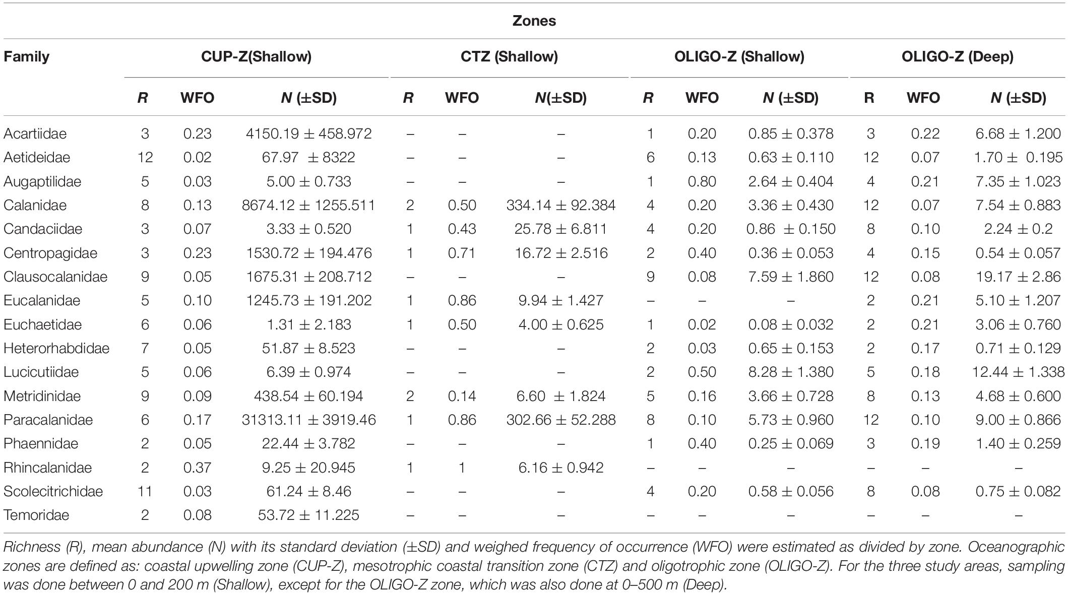
Table 1. Community descriptors for copepod families of the order Calanoida in the southeast Pacific during 2002 to 2015.

When examining the community descriptors, abundance (N), species richness (R) and weighed frequency of occurrence (WFO) for each predefined zone for the 0–200 depth strata (Table 1), it was found that much greater abundances occurred in the CUP-Z, while in the OLIGO-Z abundances were commonly 1 order of magnitude lower when compared same families. The number of species per family (family richness) tended to decrease in the OLIGO-Z in some families containing most species. This was the case for Aetideidae (14 species) and Scolecitrichidae (11 species). In most cases families had more species in the CUP-Z. However, when comparing the two depth strata within the OLIGO-Z zone, we observed greater abundance and richness at the deep stratum. This was observed in Calanidae (12 species), Aetideidae (12 species) and Paracalanidae (12 species) (Table 1).

Onshore-Offshore Distribution

For the zonal distribution analysis, we used the zonal weighed abundance (ZWA) of the families at shallow depths (0–200 m) to assess their dominant habitat across the onshore-offshore gradient. This distributional pattern is shown in Figure 2. It was found that many families can occupy the entire zonal range, although a few appeared restricted to the coastal area.

FIGURE 2

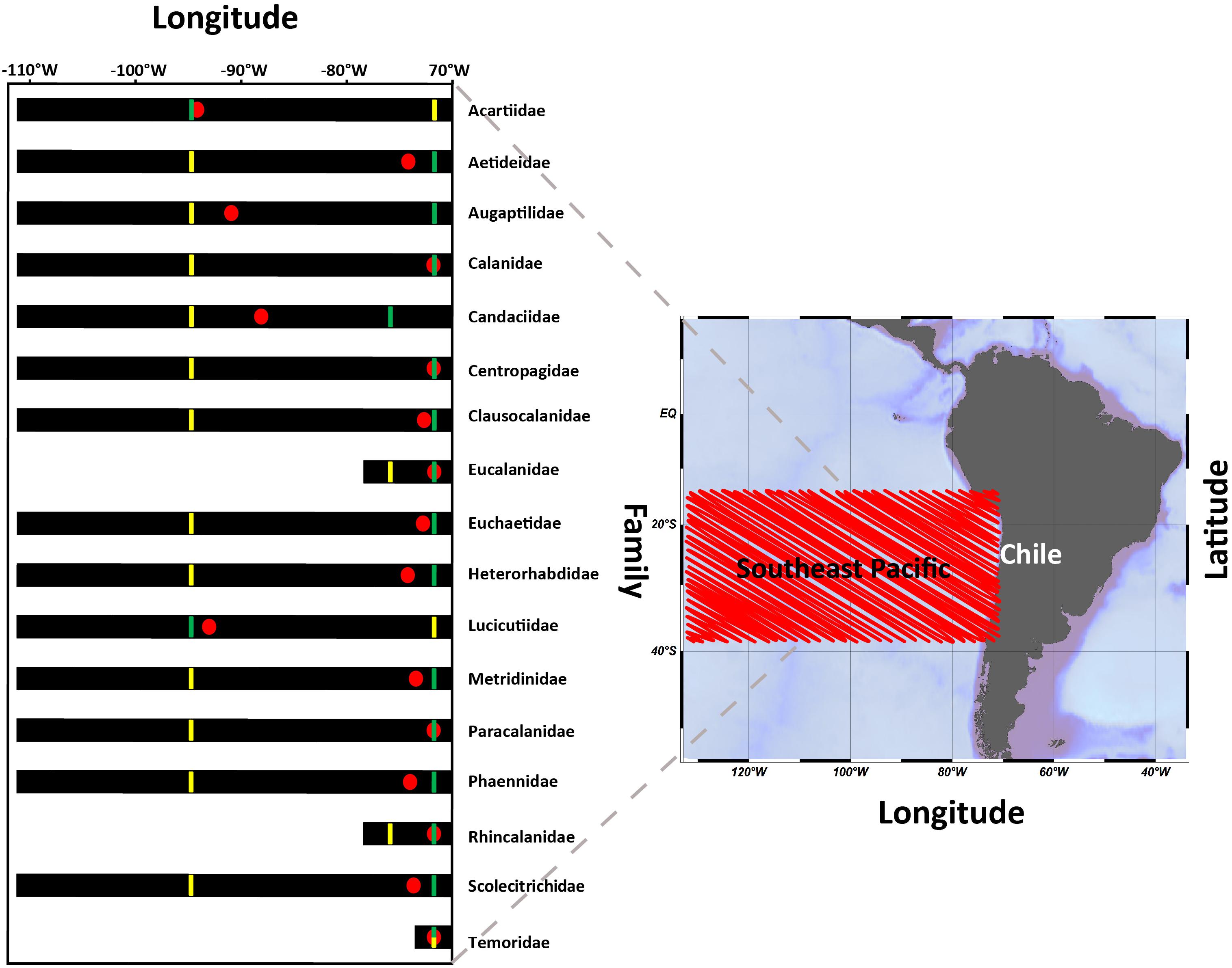
Figure 2. Mean distribution of families in the 0–200 m layer across a longitudinal gradient from the coastal zone of Chile to Easter Island, between the years 2002 and 2015. For each family, the location of the onshore-offshore weighed abundance is shown (ZWA: ), the greatest abundance (), lowest abundance () and range of distribution ().

It was also found that ZWA values were aggregated within the first 2000 km from the coast, and these varied considerably among families, although with a tendency toward the coastal zone. In any case, ZWA’s could help us to allocate dominant habitat of families, such that Acartidae, Augaptilidae, Candaciidae, and Lucicutidae which seemed to have more oceanic habitats compared to the abundant Eucalanidae, Rhincalanidae, and Temoridae, whose habitats seem centered close to shore (Figure 2). Some dominant families in the CTZ were Aetideidae, Heterohabbidae, Metridinidae, Phaennidae, and Scolecitrichidae.

In terms of absolute abundance across the onshore-offshore gradient, Figure 3 represents how families are distributed over this axis. Calanidae and Paracalanidae were the families most widely distributed (with more homogeneous distribution) across this zonal gradient and along with Acartidae and Centropagidae they were the most abundant within the CUP-Z. By contrast, Temoridae, Aetideidae, and Phaennidae were represented with much more restricted distributions (Figure 3).

FIGURE 3

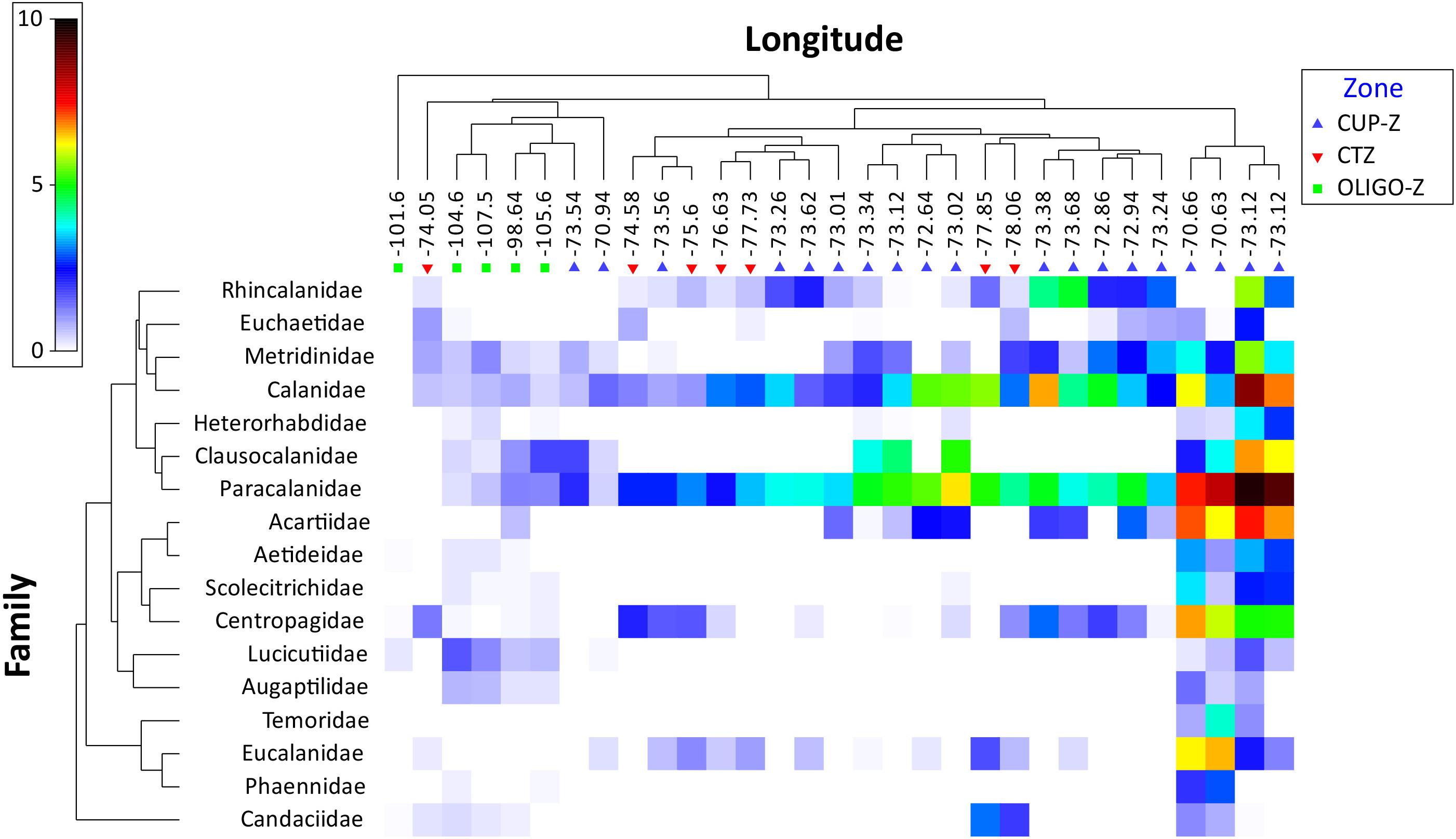
Figure 3. Shade plot of mean abundances [transformed by log (x + 1)] of the 17 families found in the 0–200 m layer, along the onshore-offshore gradient from 2002 to 2015 in the southeast Pacific. Oceanographic zones are defined as: coastal upwelling zone (CUP-Z), mesotrophic coastal transition zone (CTZ) and oligotrophic zone (OLIGO-Z). The color scale represents transformed abundance for each family.

Changes in community structure at the family level across the onshore-offshore gradient became evident after NMDS analysis using the Bray–Curtis similarity index of distance. This NMDS analysis (Figure 4A) shows that a large cluster can be arranged at 20% of similarity with most samples and significant grouping may occur at 40% of similarity where the samples of the CUP-Z zone are grouped with the others. Also, ANOSIM analysis showed significant differences in the abundance of families between the zones OLIGO-Z with CUP-Z (p-value = 0.001; Rglobal = 0.75) and CTZ (p-value 0.001; Rglobal = 0.69), but not between the zones CUP-Z and CTZ (p-value 0.14; Rglobal = 0.13).

FIGURE 4

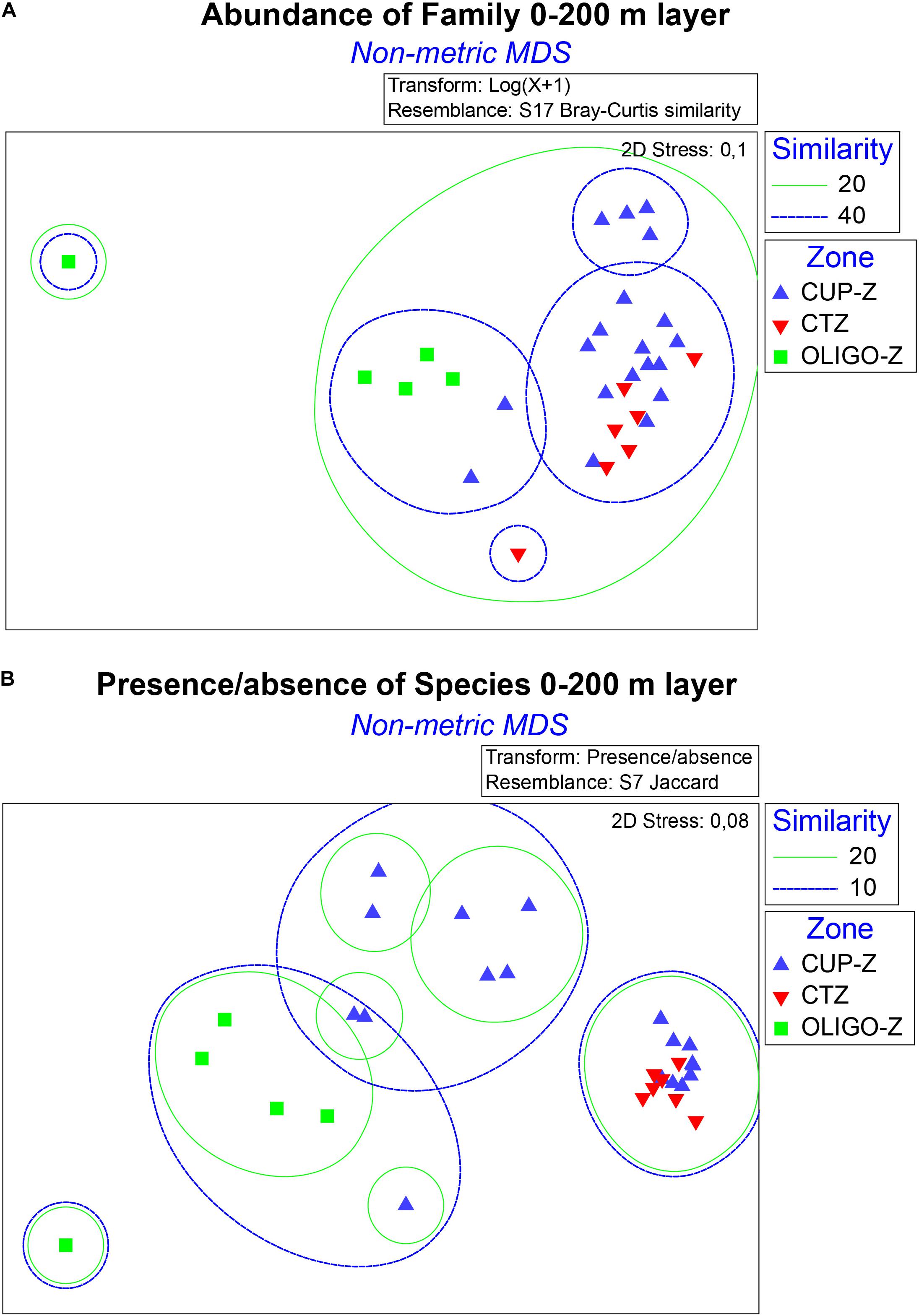
Figure 4. Non-metric multidimensional scaling diagram (NMDS) of families and species within the order Calanoida found in the 0–200 m layer, across an onshore-offshore gradient, divided in zone which were defined as: coastal upwelling zone (CUP-Z), mesotrophic coastal transition zone (CTZ) and oligotrophic zone (OLIGO-Z) of the southeast Pacific. For families NMDS (A) was calculated using its abundance through the Bray-Curtis distance index from the transformation of data with log (x + 1). For species NMDS (B) was calculated using the Jaccard distance index from the transformation of the abundance data as presence/absence of the species.

A similar analysis to that of families was applied to the community structure at the species level. In this case however, using presence or absence since abundance was too heterogeneous for comparisons. The Jaccard index of distance yielded a NMDS shown in Figure 4B. NMDS analysis revealed that at low level of similarity (10%) three groups could be observed in which, as in families, the samples from the CUP-Z zone became grouped with those from other zones. However, ANOSIM analysis at the species level showed a result similar as that observed at the family level. Significant differences were found between zones OLIGO-Z with CUP-Z (p-value 0.001; Rglobal = 0.51) and CTZ (p-value 0.001; Rglobal = 1.00). On the other hand, presence and absence of species was different between the shallow (0–200 m) and deep (0–500 m) layers (p-value = 0.001; Rglobal = 0.17) at OLIGO-Z zone. Most families exhibited a greater number of species in the deeper stratum (0–500 m), indicating that some species reside below 200 m and are not found in the shallow stratum (0–200 m).

Alongshore Distribution

When looking at the alongshore distribution of copepod families at the shallow depth stratum (0–200 m), we used a meridional weighed abundance (MWA), designed in according to our sampling area. This allowed us to allocate the dominant habitat of each family over the latitudinal axis within the CUP-Z. This alongshore pattern is shown in Figure 5. It was found that most families were widely distributed over the region, except for Rhincalanidae mostly inhabiting the southern area. Two major groups can be distinguished located either in the southern or northern portions of the study area. The southern area was characterized by seven families, Augaptilidae, Candaciidae, Centropagidae, Eucalanidae, Scolecitrichidae, and Temoridae which were the most abundant, whereas in the northern portion 10 families Calanidae, Clausocalanidae, Euchaetidae, Heterorhabditidae, Lucicutidae, Metridinidae, and Paracalanidae were well represented (Figure 5).

FIGURE 5

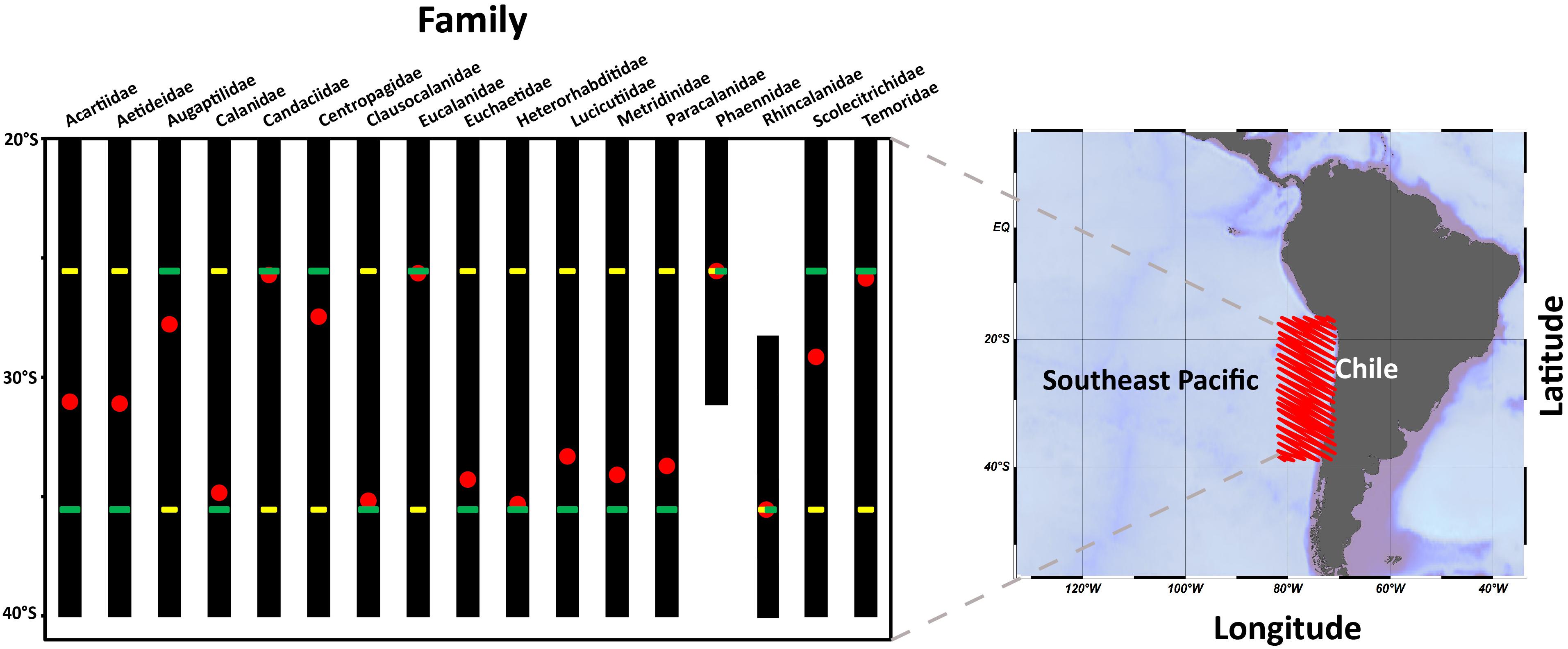
Figure 5. Mean distribution of families presents found in the 0–200 m layer across alongshore gradient from the coastal zones of Antofagasta to Concepción between 2002 and 2015. For each family the location of the alongshore weighed abundance is shown (MWA: ), range of distribution (), site of greatest abundance (), and lowest abundance ().

A shade plot (Figure 6) shows that Paracalanidae and Calanidae were widely distributed families along the upwelling zone, also representing the most abundant copepods in the region. In a lesser extent, Acartidae and Metrinidae also appeared as widely distributed, whereas other families exhibited more restricted distributions. The northern area, two families Eucalanidae (4 species) and Centropagidae (2 species) showed the highest abundances, whereas in the southern portion three families Paracalanidae (6 species), Calanidae (6 species) and Acartidae (2) presented the highest abundance values.

FIGURE 6

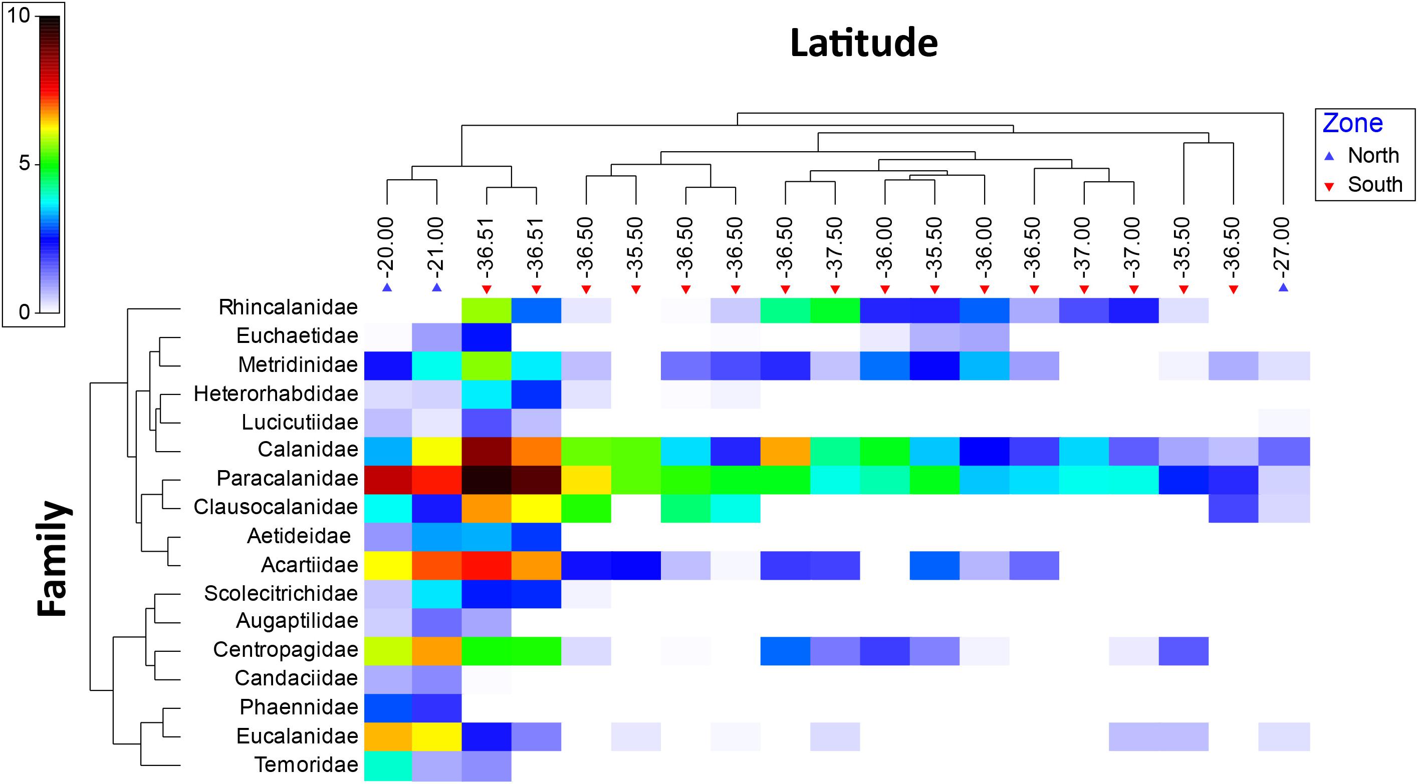
Figure 6. Shade plot of mean abundances [transformed by log (x + 1)] of the families found in the 0–200 m layer, over the north-south (alongshore) gradient from 2002 to 2015 in the southeast Pacific off the Chilean coast. Oceanographic regions were defined as north and south divided by the subtropical convergence (30°S). The color scale represents transformed abundance for each family.

Environmental Correlates

In order to examine environmental correlates of the copepod community with habitat conditions, we used the grand mean values of the study period for the different oceanographic variables (independent variables). The spatial patterns of these variables (2002–2015) are shown in Figure 7. In the CUP-Z a warmer SST in the range of 16–21°C prevails in the northern portion, while a range of 12–16°C prevails in the southern portion of this CUP-Z. The CTZ exhibits a similar northern-southern pattern and SST range as that of the CUP-Z, whereas the OLIGO-Z shows a gradual increase in SST from about 21°C up to 27°C at the northeast portion of the study area (Figure 7A). Sea surface salinity (SSS) exhibited a high variation, both over the zonal and alongshore gradients. In the CUP-Z a higher SSS in the range of 34.5–35 predominated in the northern zone, compared to a range of 33–34 observed in the southern region. The CTZ showed a similar SSS northern-southern pattern as that exhibited by the CUP-Z (Figure 7B). Contrasting with SST and SSS, the mixed layer depth MLD showed a strong variation only over the zonal gradient. In the CUP-Z the shallowest depths of MLD (<20 m) were observed, while toward the OLIGO-Z zone it shows a gradual deepening mainly in the northern portion (>80 m) (Figure 7C). Finally, Chl-a exhibited an abrupt increase of its concentration only over the zonal dimension. The highest Chl-a concentrations were observed in the CUP-Z zone (>1 mg m^–3), while toward the OLIGO-Z zone the concentration was extremely low (<0.05 mg m^–3) (Figure 7D).

FIGURE 7

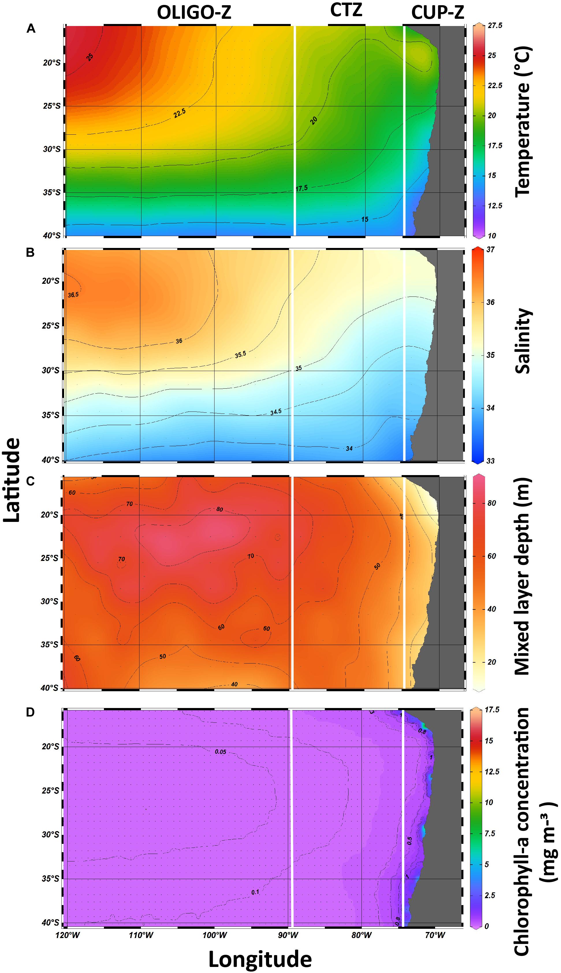
Figure 7. Satellite-derived means of surface oceanographic conditions in the southeast Pacific from 2002 to 2015 for the three study areas defined as: coastal upwelling zone (CUP-Z), mesotrophic coastal transition zone (CTZ), and oligotrophic zone (OLIGO-Z). (A) temperature, (B) salinity, (C) mixed layer, and (D) Chlorophyll-a concentration.

Spatial patterns of SST gradients over the zonal and alongshore axes are shown in Figure 8. The Southeast Pacific showed strong temperature gradients within and across all predefined regions for the study period. The zonal gradient exhibited a very particular spatial pattern, characterized by bands nearly parallel to the coast of about 700–900 km width. These features showed stronger gradients (>0.4°C), in the region between 80° and 70°W, corresponding mainly to the CTZ off the coastal upwelling area (Figure 8A). The alongshore gradient presented a zone of lower variability (<0.2°C) between 20–30°, while toward the southern portion an intensification of this gradient was observed and the differentiation between these two patterns became evident at 30°S corresponding to the subtropical convergence (Figure 8B).

FIGURE 8

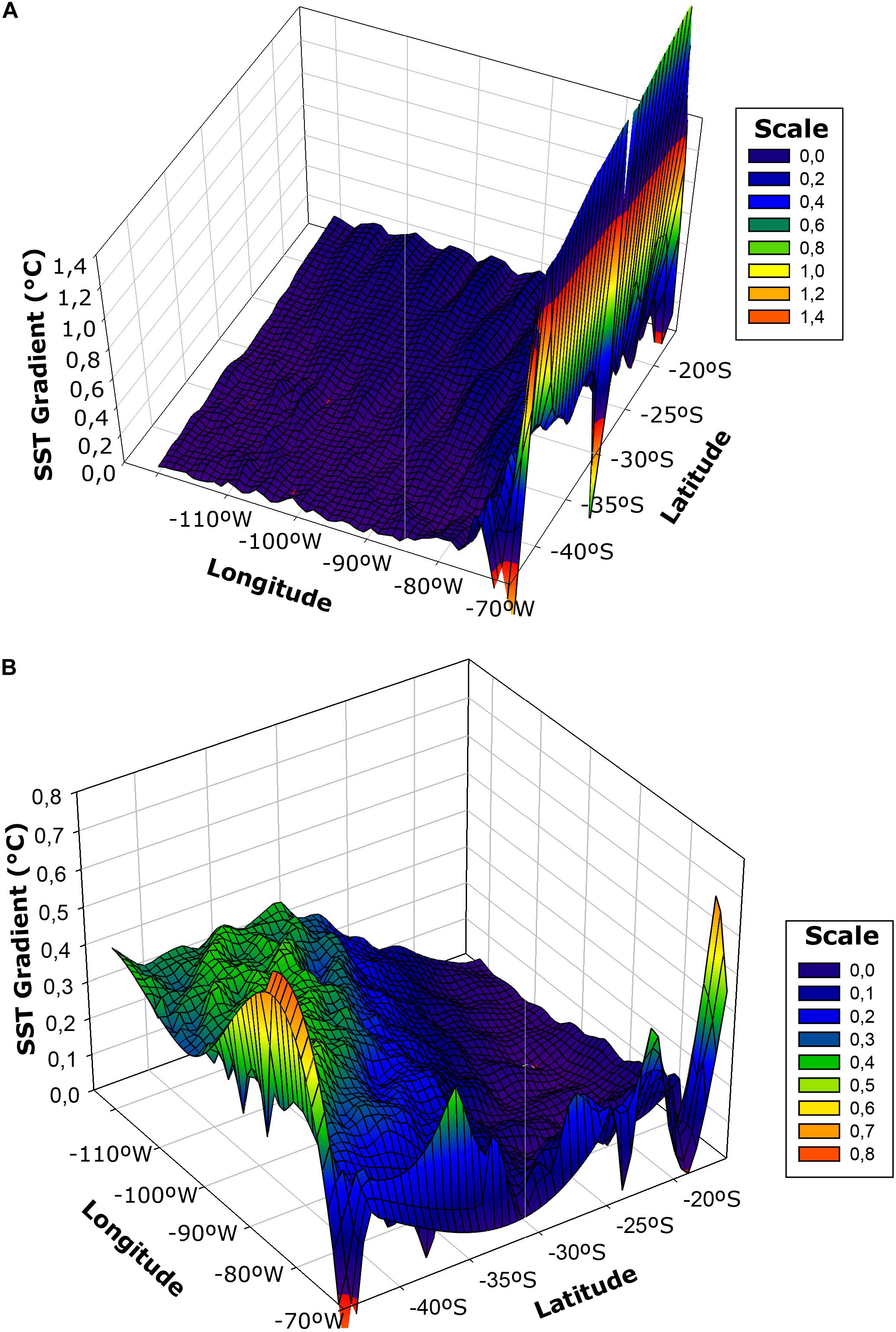
Figure 8. Spatial gradients of sea surface temperature (SST) for the onshore-offshore (Zonal) (A) and the alongshore (meridional) (B) gradients in the southeast Pacific for the period 2002–2015. Gradient resolution is for 1° from mean monthly values of SST.

The multivariate analysis between the abiotic and biotic variables (families and species) was performed with the family and species matrices. In both cases similar results were found. The BIOENV analysis between oceanographic variables and the abundances of families and species showed a high correlation with SST (families: r = 0.5 and species: r = 0.6) (Supplementary Table S6). Indeed, DISTLM analysis indicated that the three variables SST, MLD and Chl-a correlate significantly with the abundance of both species and families (p-value < 0.05), although SST explained the highest percentage of variability in the community matrix (families: 21% and species: 20%). Furthermore, the sequential test with the stepwise procedure selected the SST and MLD as the variables that best explain the variation in the species matrix, for the selection of the best model, the lowest value of the AIC was used. More detailed results from this analysis are shown in Supplementary Tables S7, S8.

When looking for a predictive model for copepod diversity, it was found that most oceanographic variables had a significant effect on family and species richness at the shallow depth stratum, as resulting from application of a Generalized Additive Models (GAMs). Over the zonal gradient we found from the AIC value, as the most parsimonious criteria for best-fit GAMs, that a predictive model incorporated SST and MLD to explain both the family and species richness (Table 2). Relationships between family richness with SST and MLD explained together a 39.80% of the variance (Table 2). These effects were highly significant (P-value < 0.01) and showed a positive relationship with the SST, and a negative relationship with MLD (Figures 9A,B). At species level, it was observed that variation in richness was explained in 29.10% by both SST and MLD (Table 2). However, only SST exhibited a significant and positive effect on richness (Figures 10A,B).

TABLE 2

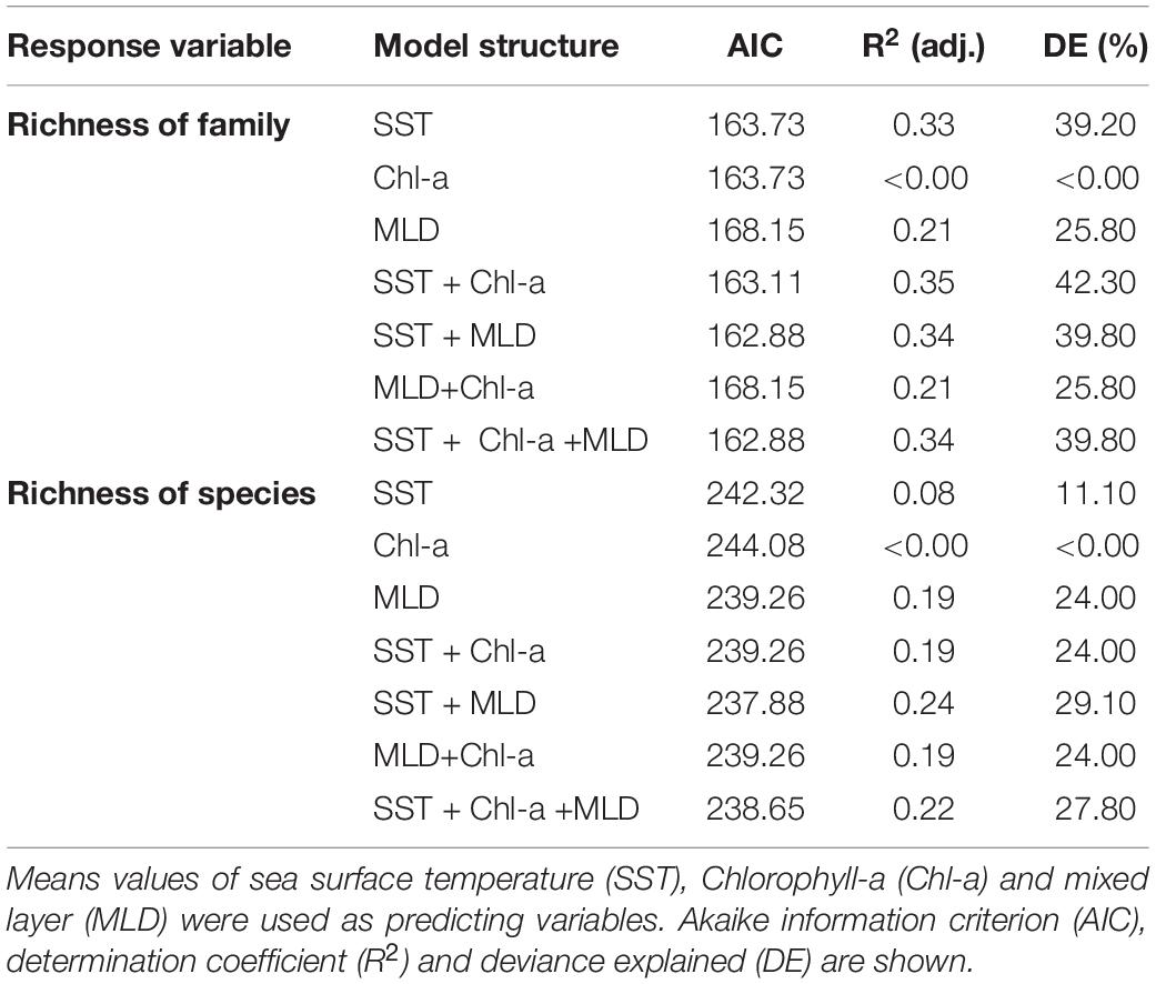
Table 2. Generalized additive models (GAM_s) after fitting the relationship found in the 0–200 m layer, between family and species richness of calanoid copepods and oceanographic variables at Southeast Pacific, for the period 2002–2015 over an onshore-offshore (zonal) gradient.

FIGURE 9

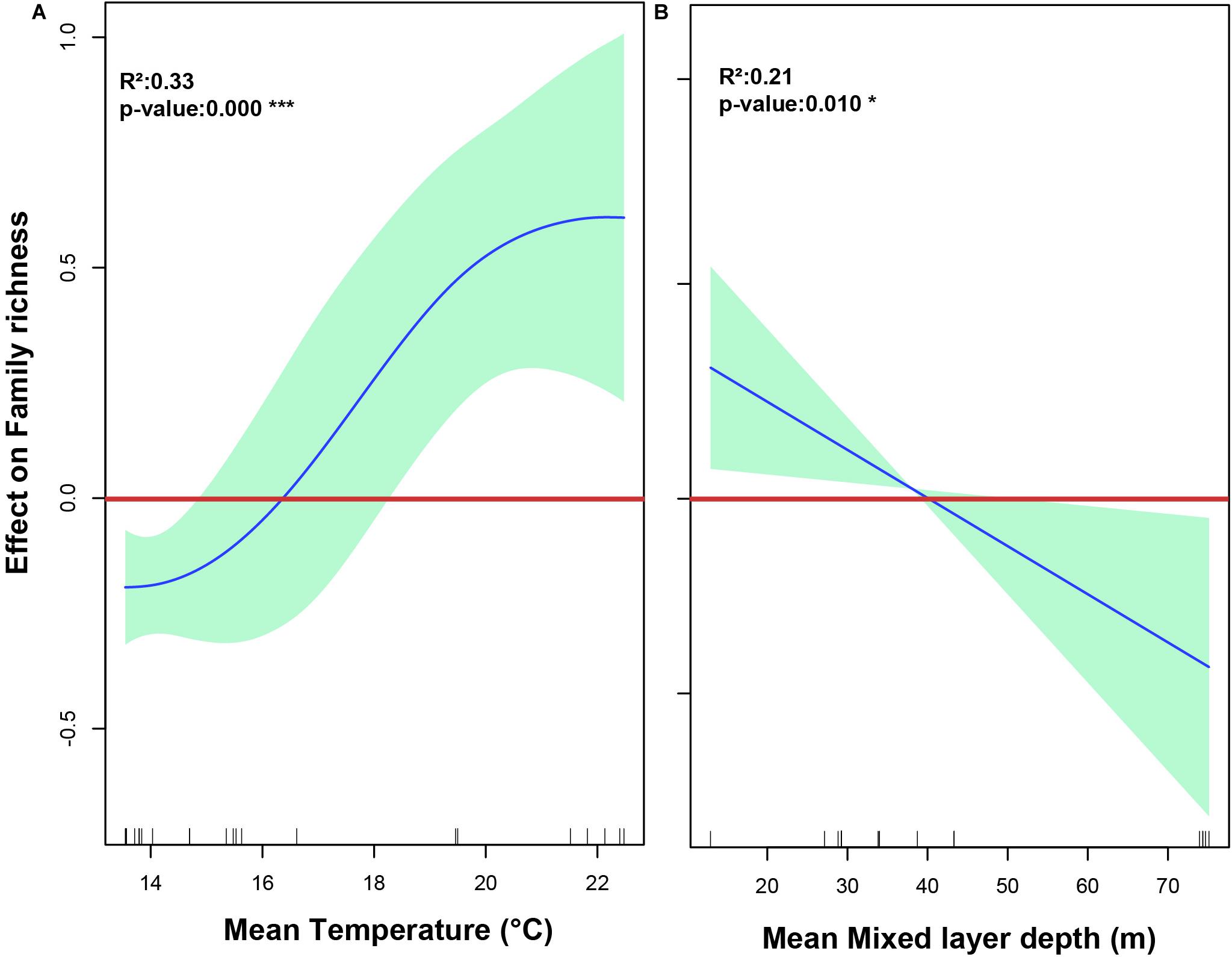
Figure 9. The relationship between oceanographic variables and family richness of calanoid copepods found in the 0–200 m layer in the southeast Pacific, as represented by a generalized additive model (GAM). (A) The effect of Mean sea surface temperature on family richness. (B) The effect of mean depth of the mixed layer on family richness. Spline fit (solid blue line) is bound at 95% confidence intervals (light green area). Values > 0 indicate a positive effect on richness, values < 0 indicate a negative effect. The rug plot (dashes above the x-axis) represents the distribution of data points.

FIGURE 10

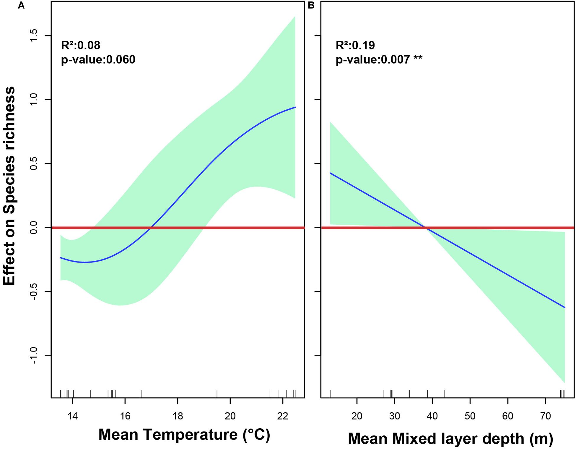
Figure 10. The relationship between oceanographic variables and species richness of calanoid copepods found in the 0–200 m layer in the southeast Pacific, as represented by a generalized additive model (GAM). (A) The effect of Mean sea surface temperature on species richness. (B) The effect of mean depth of the mixed layer on species richness. Spline fit (solid blue line) is bound at 95% confidence intervals (light green area). Values > 0 indicate a positive effect on richness, values < 0 indicate a negative effect. The rug plot (dashes above the x-axis) represents the distribution of data points.

Discussion

Biological diversity of zooplankton can be modulated by environmental gradients which modify the spatial patterns of species and communities (Lawton, 1999; Hillebrand and Azovsky, 2001; Rex et al., 2001). Although the partition of the habitat over the horizontal plane of zooplankton communities has been reported in some works (e.g., Heinrich, 1973; Gonzalez and Marín, 1998; Escribano and Hidalgo, 2000; Linacre and Palma, 2004), there have been difficulties for identifying and understanding the mechanisms that modulate differential distributions. In this context, our analyses revealed a high structuring of the order Calanoida, linked to spatial zonation, both in zonal and meridional gradient. However, some sources of variance may introduce biases affecting the observed species distributions. For example, sampling depth can modify the observed horizontal distribution of copepods (e.g., Judkins, 1980), and even though we separated samplings done over different depth strata, variability introduced by vertical distribution, including vertical migrations become difficult to account in our horizontal analyses. Also, most of the samplings were made in the CUP-Z targeting the upper 200 m, which is the zone where most species of copepods aggregate due to vertical restrictions imposed by presence of a shallow oxygen minimum zone (Escribano et al., 2009). Another additional source of variation could be caused by using different sampling gear. In our case, we selected the same mesh size for the zooplankton nets, but different opening diameter of nets and variable towing speed may have occurred. For instance, a comparison of two type of gear, the MOCNESS and WP2 nets, showed that estimates of biomasses differed between these nets, although such differences were mostly accounted by the largest fractions of zooplankton represented by euphausiids and amphipods, and there was no evidence for a significant effect of net opening diameter in the estimates of abundance of smaller organisms, such as copepods (Gjøsæter et al., 2000). In our analyses we did not find significant differences in copepods abundances estimated by two different sampling gears, Tucker trawl and Multinet and it seems that both devices can properly sample mesozooplankton which was our target group. This result agrees with a previous study in which different vertical, oblique, and multiple opening/closing net systems resulted in similar estimates of zooplankton with comparable mesh-sized nets and a sufficiently high ratio of mesh to mouth opening (Skjoldal et al., 2013).

Samples analyzed in this study were obtained in different years and seasons. The coastal transition and oligotrophic zones were sampled during spring-summer, unlike the coastal region (upwelling zone) which was sampled throughout the year, such that it was then possible to assess the effect of seasonality on the species composition and families. Even although, for the coastal zone it has been reported an effect of seasonal variability on the composition of species (Hidalgo and Escribano, 2001; Escribano et al., 2007), we did not detect such effect when evaluating composition of families. This lack of seasonality effect could be explained by continued presence of copepod families, although eventually represented by different species, or different stages of same species, so that showing a lack of variability in the total abundance and diversity at different times of the year. Continuous reproduction and multigenerational populations can also help explain species occurrence year-round (Escribano and McLaren, 1999; Hidalgo and Escribano, 2007).

With respect to zonation over the zonal gradient, as found in the composition of families and species of the order Calanoida, we found highly significant changes from the coastal upwelling to the oligotrophic zones. Other works in the same area also reported changes in species composition; example for euphausiids (Riquelme-Bugueño et al., 2012) and (Palma and Silva, 2006). One of the main explanations for this pattern is attributed to the presence of different water masses, although variable sources of food and nutrient over this gradient has also been suggested, providing distinctive characteristics to each of the study zones (Silva et al., 2009; González et al., 2019). The costal upwelling zone is mainly influenced by Equatorial Subsurface Water, characterized by a high concentration of nutrients and source of fresh carbon from the atmosphere that is rapidly transferred to copepods (Morales et al., 1996; Gruber et al., 1999; Daneri et al., 2000; Silva and Valdenegro, 2003; Mompeán et al., 2013).However, mesotrophic coastal transition and oligotrophic zones are composed by Sub Antarctic Water and Subtropical Water, respectively, which present lower concentrations of nutrients and more regenerated carbon sources compared to the coastal zone (Reid, 1973; Nakatsuka et al., 1992). All these factors along with presence of the anticyclonic gyre in oceanic region can isolates species assemblages from the adjacent areas, and so promoting a semi-closed ecosystem regulated by in situ processes (McGowan, 1971, 1977). Over a longer time-scale samples of marine microfossils collected during the Pleistocene indicate that the longitudinal zonation observed in Southern Pacific persisted allowing to observe the structuring patterns at the level of family and species of calanoid copepods (Riedel and Funnell, 1964).

A high degree of structuring can also be observed over the alongshore gradient, with spatial agreement between analyses done at the levels of both species and families, showing the presence of three groups distributed in the north, a transition region, and the south. Other works done about the same gradient have also reported the presence of these biogeographic breaks in other organisms such as kelps, and bivalves mollusks (Broitman et al., 2001; Cárdenas et al., 2009; González et al., 2012). The boundaries of these biogeographic regions are not fixed and can vary seasonally and between years (Escribano et al., 2003). Despite that the limits between the different regions are not clear, it has been reported that the transition region shows a high correlation with a gradient of surface temperature (Broitman et al., 2001), irregular patterns of circulation (Hormazabal et al., 2004), and a sharp narrowing of the continental shelf (Strub et al., 1998). Furthermore, the presence and interaction of different water masses, such as: equatorial subsurface water and intermediate Antarctic water, can be the source for equatorial species in the north region and polar/sub-Antarctic in the south, possibly generating a transition zone between 30°S corresponding to tropical (Escribano et al., 2003; Hidalgo et al., 2010).

In this study we report a strong dependence of richness with temperature both at family and species levels. In this respect, it is known that temperature can modify the rates of various biological processes in copepods, such as growth, productivity and mortality, but also influencing physical conditions of the water column, such as stratification and availability of nutrients and indirectly affecting the ecology of copepods (Reese et al., 2005; Kiørboe and Hirst, 2008). Along the zonal gradient it was observed a notorious increase in mean temperature from the coastal zone to the open ocean associated with increasing richness of copepod families. In fact, mean temperature was strongly correlated (ca. 29–39%) with richness both of families and species levels and a positive correlation with temperatures values > 17°C due to the presence of Subtropical Water (Silva et al., 2009). In several regions of the world a positive correlation between temperature and richness of aquatic zooplankton species has been reported, accompanied by a decrease in abundance (Matsubara, 1993; Castro et al., 2007; Hessen et al., 2007) and with marine organisms at a global scale as well (Antão et al., 2020). Regarding the alongshore gradient we observed that temperature showed a significant effect on species richness and this can be associated with rapid and abrupt change of temperature between 20 and 30°S in the coastal zone due to a spatial variation in the seasonal upwelling regime between northern Chile and southern Chile (Escribano et al., 2004), and presence of different water masses (Silva et al., 2009). The onshore-offshore (zonal) gradient of SST indeed revealed the existence of discrete habitats imposing constraints for population connectivity of epipelagic plankton. These physical barriers can play a significant role for evolutionary processes and gene flow across this zonal gradient, as shown by a recent work revealing ongoing speciation in the cosmopolitan copepod Pleuromamma abdominalis over this gradient (González et al., 2020). Such processes can certainly be extended to the community level and so influencing both family and species richness.

In addition to temperature, many other factors may influence zooplankton diversity patterns (Angel, 1997 for review). For instance, in the Benguela biome it has been suggested that variation in primary production (PP) and the coupling between primary producer and secondary producer may be the main controllers of the copepod community structure (Woodd-Walker et al., 2002). In our work, Chl-a as a proxy of food or ocean productivity, did not show any correlation with copepods diversity and species distribution. In this regard, the spatial scale is an important issue to consider and it may be that local (patchiness) effects of food resources can indeed influence species distribution and composition. However, over a large, basin scale physical barriers, such as those formed by temperature gradients, and the temperature within them are key drivers for diversity patterns. Depth of the mixed layer also deserves further attention. In the coastal zone vertical distribution, commonly restricted by strong gradients in temperature, oxygen, light or other factors, the available habitat becomes spatially limited, and deepening of the mixed layer which also correlates positively with temperature may help expanding the vertical and so promoting increased diversity (Tittensor et al., 2010; Mora et al., 2011).

In any case, temperature and its spatial arrangements have been reported as a major correlate of zooplankton diversity in other studies as well (Rombouts et al., 2009; Beaugrand and Kirby, 2010), implying that (Hessen et al., 2007) ongoing warming of the ocean may greatly impact copepod diversity patterns by either altering their comfort ranges of temperature or by modifying the spatial gradients.

Data Availability Statement

The datasets analyzed for this study have been deposited in the Southeast Regional Node of OBIS [https://ron.udec.cl/].

Author Contributions

All co-authors have contributed to the work. CG contributed to data analysis and writing. RE integrated the all results and developed the direction of the manuscript. JM-M and RE participated in discussion and data analyses and commented on the manuscript. All the authors contributed to the article and approved the submitted version.

Conflict of Interest

The authors declare that the research was conducted in the absence of any commercial or financial relationships that could be construed as a potential conflict of interest.

Funding

This work was funded by Grants CIMAR-21 and CIMAR-22 of CONA-Chile and the Millennium Institute of Oceanography (ICN12_019-IMO). Additional funding was provided by Grant FONDECYT 188-1682. CG work was supported by the CONICYT Scholarship No 21160714.

Acknowledgments

We thank to the two reviewers for their valuable and key comments that greatly improved the work. We are also grateful to Daniel Toledo for sampling assistance during most cruises.

Supplementary Material

The Supplementary Material for this article can be found online at: https://www.frontiersin.org/articles/10.3389/fevo.2020.554409/full#supplementary-material

Footnotes

1. ^ https://obis.org/
2. ^ http://apdrc.soest.hawaii.edu/projects/argo/
3. ^ https://podaac.jpl.nasa.gov
4. ^ http://oaflux.whoi.edu/heatflux.html

References

Andersen, V., Devey, C., Gubanova, A., Picheral, M., Melnikov, V., Tsarin, S., et al. (2004). Vertical distributions of zooplankton across the Almeria-Oran frontal zone (Mediterranean Sea). J. Plankton Res. 26, 275–293. doi: 10.1093/plankt/fbh036

PubMed Abstract | CrossRef Full Text | Google Scholar

Anderson, M. (2008). Permanova+ for Primer?: guide to software and statisticl methods. Plymouth: PRIMER-E Ltd.

Google Scholar

Angel, M. V. (1997). Pelagic biodiversity. Mar. Biodivers. patterns Process. Cambridge, UK: Cambridge Univ. Press. doi: 10.1017/CBO9780511752360.004

CrossRef Full Text | Google Scholar

Antão, L. H., Bates, A. E., Blowes, S. A., Waldock, C., Supp, S. R., Magurran, A. E., et al. (2020). Temperature-related biodiversity change across temperate marine and terrestrial systems. Nat. Ecol. Evol. 4, 927–933. doi: 10.1038/s41559-020-1185-7

PubMed Abstract | CrossRef Full Text | Google Scholar

Aronés, K., Ayón, P., Hirche, H.-J., and Schwamborn, R. (2009). Hydrographic structure and zooplankton abundance and diversity off Paita, northern Peru (1994 to 2004)—ENSO effects, trends and changes. J. Mar. Syst. 78, 582–598. doi: 10.1016/j.jmarsys.2009.01.002

CrossRef Full Text | Google Scholar

Beaugrand, G. (2003). Long-term changes in copepod abundance and diversity in the north-east Atlantic in relation to fluctuations in the hydroclimatic environment. Fish Oceanogr. 12, 270–283. doi: 10.1046/j.1365-2419.2003.00248.x

CrossRef Full Text | Google Scholar

Beaugrand, G., and Kirby, R. (2010). Spatial changes in the sensitivity of Atlantic cod to climate-driven effects in the plankton. Clim. Res. 41, 15–19. doi: 10.3354/cr00838

CrossRef Full Text | Google Scholar

Beaugrand, G., Reid, P. C., Ibañez, F., Lindley, J. A., and Edwards, M. (2002). Reorganization of North Atlantic marine copepod biodiversity and climate. Science. 296, 1692–1694. doi: 10.1126/science.1071329

PubMed Abstract | CrossRef Full Text | Google Scholar

Bonnet, S., Guieu, C., Bruyant, F., Pr, O., Wambeke, F., Van Raimbault, P., et al. (2008). Nutrient limitation of primary productivity in the Southeast Pacific (BIOSOPE cruise). Biogeosciences 5, 215–225. doi: 10.5194/bg-5-215-2008

CrossRef Full Text | Google Scholar

Broitman, B., Navarrete, S., Smith, F., and Gaines, S. (2001). Geographic variation of southeastern Pacific intertidal communities. Mar. Ecol. Prog. Ser. 224, 21–34. doi: 10.3354/meps224021

CrossRef Full Text | Google Scholar

Cárdenas, L., Castilla, J. C., and Viard, F. (2009). A phylogeographical analysis across three biogeographical provinces of the south-eastern Pacific: the case of the marine gastropod Concholepas concholepas. J. Biogeogr. 36, 969–981. doi: 10.1111/j.1365-2699.2008.02056.x

CrossRef Full Text | Google Scholar

Castro, L. R., Troncoso, V. A., and Figueroa, D. R. (2007). Fine-scale vertical distribution of coastal and offshore copepods in the Golfo de Arauco, central Chile, during the upwelling season. Prog. Oceanogr. 75, 486–500. doi: 10.1016/j.pocean.2007.08.012

CrossRef Full Text | Google Scholar

Crame, J. A. (1993). Latitudinal range fluctuations in the marine realm through geological time. Trends Ecol. Evol. 8, 162–166. doi: 10.1016/0169-5347(93)90141-B

CrossRef Full Text | Google Scholar

Cronin, T. M., and Schneider, C. E. (1990). Climatic influences on species: evidence from the fossil record. Trends Ecol. Evol. 5, 275–279. doi: 10.1016/0169-5347(90)90080-W

CrossRef Full Text | Google Scholar

Daneri, G., Dellarossa, V., Quiñones, R., Jacob, B., Montero, P., and Ulloa, O. (2000). Primary production and community respiration in the Humboldt Current System off Chile and associated oceanic areas. Mar. Ecol. Prog. Ser. 197, 41–49. doi: 10.3354/meps197041

CrossRef Full Text | Google Scholar

Escribano, R., Daneri, G., Farías, L., Gallardo, V. A., González, H. E., Gutiérrez, D., et al. (2004). Biological and chemical consequences of the 1997–1998 El Niño in the Chilean coastal upwelling system: A synthesis. Deep. Res. Part II Top. Stud. Oceanogr. 51, 2389–2411. doi: 10.1016/j.dsr2.2004.08.011

CrossRef Full Text | Google Scholar

Escribano, R., Fernández, M., and Aranís, A. (2003). Physical-chemical processes and patterns of diversity of the Chilean eastern boundary pelagic and benthic marine ecosystems: an overview. Gayana 67, 190–205. doi: 10.4067/S0717-65382003000200008

PubMed Abstract | CrossRef Full Text | Google Scholar

Escribano, R., and Hidalgo, P. (2000). Spatial distribution of copepods in the north of the Humboldt Current region off Chile during coastal upwelling. J. Mar. Biol. Assoc. UK 80, 283–290. doi: 10.1017/S002531549900185X

CrossRef Full Text | Google Scholar

Escribano, R., Hidalgo, P., González, H., Giesecke, R., Riquelme-Bugueño, R., and Manríquez, K. (2007). Seasonal and inter-annual variation of mesozooplankton in the coastal upwelling zone off central-southern Chile. Prog. Oceanogr. 75, 470–485. doi: 10.1016/j.pocean.2007.08.027

CrossRef Full Text | Google Scholar

Escribano, R., Hidalgo, P., and Krautz, C. (2009). Zooplankton associated with the oxygen minimum zone system in the northern upwelling region of Chile during March 2000. Deep Sea Res. Part II Top. Stud. Oceanogr. 56, 1083–1094. doi: 10.1016/j.dsr2.2008.09.009

CrossRef Full Text | Google Scholar

Escribano, R., and McLaren, I. (1999). Production of Calanus chilensis in the upwelling area of Antofagasta, northern Chile. Mar. Ecol. Prog. Ser. 177, 147–156. doi: 10.3354/meps177147

CrossRef Full Text | Google Scholar

Gee, J. H. R. (1991). Speciation and biogeography. Fundam. Aquat. Ecol. 1991, 172–185. doi: 10.1002/9781444314113.ch9

CrossRef Full Text | Google Scholar

Gewin, V. (2010). Dead in the water. Nature 466:812. doi: 10.1038/466812a

PubMed Abstract | CrossRef Full Text | Google Scholar

Gjøsæter, H., Dalpadado, P., Hassel, A., and Skjoldal, H. R. (2000). A comparison of performance of WP2 and MOCNESS. J. Plankton Res. 22, 1901–1908. doi: 10.1093/plankt/22.10.1901

PubMed Abstract | CrossRef Full Text | Google Scholar

González, A., Beltrán, J., Hiriart-Bertrand, L., Flores, V., de Reviers, B., Correa, J. A., et al. (2012). Identification of cryptic species in the Lessonia nigrescens complex (phaeophyceae, laminariales) ¹. J. Phycol. 48, 1153–1165. doi: 10.1111/j.1529-8817.2012.01200.x

PubMed Abstract | CrossRef Full Text | Google Scholar

Gonzalez, A., and Marín, V. (1998). Distribution and life cycle of Calanus chilensis and Centropages brachiatus (Copepoda) in Chilean coastal waters:a GIS approach. Mar. Ecol. Prog. Ser. 165, 109–117. doi: 10.3354/meps165109

CrossRef Full Text | Google Scholar

González, C. E., Escribano, R., Bode, A., and Schneider, W. (2019). Zooplankton Taxonomic and Trophic Community Structure Across Biogeochemical Regions in the Eastern South Pacific. Front. Mar. Sci. 5:00498. doi: 10.3389/fmars.2018.00498

CrossRef Full Text | Google Scholar

González, C. E., Goetze, E., Escribano, R., Ulloa, O., and Victoriano, P. (2020). Genetic diversity and novel lineages in the cosmopolitan copepod Pleuromamma abdominalis in the Southeast Pacific. Sci. Rep. 10, 1–15. doi: 10.1038/s41598-019-56935-5

PubMed Abstract | CrossRef Full Text | Google Scholar

Gruber, N., Keeling, C. D., Bacastow, R. B., Guenther, P. R., Lueker, T. J., Wahlen, M., et al. (1999). Spatiotemporal patterns of carbon-13 in the global surface oceans and the oceanic suess effect. Glob. Biogeochem. Cycles 13, 307–335. doi: 10.1029/1999GB900019

CrossRef Full Text | Google Scholar

Heinrich, A. K. (1973). Horizontal distribution of copepods in the Peru current region. Oceanology 13, 97–103.

Google Scholar

Hessen, D. O., Bakkestuen, V., and Walseng, B. (2007). Energy Input and Zooplankton Species Richness. Ecography 30, 749–758. doi: 10.1111/j.2007.0906-7590.05259.x

CrossRef Full Text | Google Scholar

Hidalgo, P., and Escribano, R. (2001). Succession of pelagic copepod species in coastal waters off northern Chile: The influence of the 1997–98 El Niño. Hydrobiologia 45, 153–160. doi: 10.1023/A:1013188522222

CrossRef Full Text | Google Scholar

Hidalgo, P., and Escribano, R. (2007). Coupling of life cycles of the copepods Calanus chilensis and Centropages brachiatus to upwelling induced variability in the central-southern region of Chile. Prog. Oceanogr. 75, 501–517. doi: 10.1016/j.pocean.2007.08.028

CrossRef Full Text | Google Scholar

Hidalgo, P., Escribano, R., Vergara, O., Jorquera, E., Donoso, K., and Mendoza, P. (2010). Patterns of copepod diversity in the Chilean coastal upwelling system. Deep. Res. Part II Top. Stud. Oceanogr. 57, 2089–2097. doi: 10.1016/j.dsr2.2010.09.012

CrossRef Full Text | Google Scholar

Hillebrand, H., and Azovsky, A. I. (2001). Body size determines the strength of the latitudinal diversity gradient. Ecography 24, 251–256. doi: 10.1111/j.1600-0587.2001.tb00197.x

CrossRef Full Text | Google Scholar

Hormazabal, S., Shaffer, G., and Leth, O. (2004). Coastal transition zone off Chile. J. Geophys. Res. C Ocean 109:1956. doi: 10.1029/2003JC001956

CrossRef Full Text | Google Scholar

Judkins, D. C. (1980). Vertical distribution of zooplankton in relation to the oxygen minimum off Peru. Deep Sea Res. Part A, Oceanogr. Res. Pap. 27, 475–487. doi: 10.1016/0198-0149(80)90057-6

CrossRef Full Text | Google Scholar

Kiørboe, T., and Hirst, A. (2008). Optimal development time in pelagic copepods. Mar. Ecol. Prog. Ser. 367, 15–22. doi: 10.3354/meps07572

CrossRef Full Text | Google Scholar

Kletou, D., and Hall-Spencer, M. J. (2012). Threats to Ultraoligotrophic Marine Ecosystems. London: InTech. doi: 10.5772/34842

CrossRef Full Text | Google Scholar

Lawton, J. H. (1999). Are There General Laws in Ecology? Oikos 84:177. doi: 10.2307/3546712

CrossRef Full Text | Google Scholar

Lenz, P. H. (2012). The biogeography and ecology of myelin in marine copepods. J. Plankton Res. 34, 575–589. doi: 10.1093/plankt/fbs037

PubMed Abstract | CrossRef Full Text | Google Scholar

Linacre, L., and Palma, S. (2004). Variabilidad espacio-temporal de los eufáusidos frente a la costa de Concepción. Chile. Investig. Mar. 32, 19–32. doi: 10.4067/S0717-71782004000100003

PubMed Abstract | CrossRef Full Text | Google Scholar

Mann, K. H., and Lazier, J. R. N. (2013). Dynamics of marine ecosystems: biological-physical interactions in the oceans. Berlin: Springer.

Google Scholar

Matsubara, T. (1993). Rotifer community structure in the south basin of Lake Biwa. Hydrobiologia 271, 1–10. doi: 10.1007/BF00005690

CrossRef Full Text | Google Scholar

McClain, C. R., and Barry, J. P. (2010). Habitat heterogeneity, disturbance, and productivity work in concert to regulate biodiversity in deep submarine canyons. Ecology 91, 964–976. doi: 10.1890/09-0087.1

CrossRef Full Text | Google Scholar

McGowan, J. A. (1971). “Oceanic biogeography of the Pacific,” in The micropaleontology of the oceans, eds B. M. Funnel and W. R. Reidel (Cambridge: Cambridge University Press), 3–74.

Google Scholar

McGowan, J. A. (1977). “What regulates pelagic community structure in the Pacific?,” in Oceanic sound scattering prediction, eds N. R. Andersen and B. J. Zahuranec (New York, NY: Plenum Press), 423–443.

Google Scholar

Molfino, B. (1994). Palaeoecology of marine systems. Aquat. Ecol. Scale, pattern Process. Cambridge: Blackwell Sci. Publ, 517–546.

Google Scholar

Mompeán, C., Bode, A., Benítez-Barrios, V. M., Domínguez-Yanes, J. F., José, E., and Fraile-Nuez, E. (2013). Spatial patterns of plankton biomass and stable isotopes reflect the influence of the nitrogen-fixer Trichodesmium along the subtropical North Atlantic. J. Plankton Res. 35:011. doi: 10.1093/plankt/fbt011

PubMed Abstract | CrossRef Full Text | Google Scholar

Mora, C., Tittensor, D. P., Adl, S., Simpson, A. G. B., and Worm, B. (2011). How Many Species Are There on Earth and in the Ocean? PLoS Biol. 9:e1001127. doi: 10.1371/journal.pbio.1001127

PubMed Abstract | CrossRef Full Text | Google Scholar

Morales, C. E., Blanco, J. L., Braun, M., Reyes, H., and Silva, N. (1996). Chlorophyll-a distribution and associated oceanographic conditions in the upwelling region off northern Chile during the winter and spring 1993. Deep Sea Res. Part I Oceanogr. Res. Pap. 43, 267–289. doi: 10.1016/0967-0637(96)00015-5

CrossRef Full Text | Google Scholar

Morel, A., Claustre, H., and Gentili, B. (2010). The most oligotrophic subtropical zones of the global ocean: Similarities and differences in terms of chlorophyll and yellow substance. Biogeosciences 7, 3139–3151. doi: 10.5194/bg-7-3139-2010

CrossRef Full Text | Google Scholar

Nakatsuka, T., Handa, N., Wada, E., and Wong, C. S. (1992). The dynamic changes of stable isotopic ratios of carbon and nitrogen in suspended and sedimented particulate organic matter during a phytoplankton bloom. J. Mar. Res. 50, 267–296. doi: 10.1357/002224092784797692

CrossRef Full Text | Google Scholar

Palma, S., and Silva, N. (2006). Epipelagic siphonophore assemblages associated with water masses along a transect between Chile and Easter Island (eastern South Pacific Ocean). J. Plankton Res. 28, 1143–1151. doi: 10.1093/plankt/fbl044

PubMed Abstract | CrossRef Full Text | Google Scholar

Peijnenburg, K. T. C. A., and Goetze, E. (2013). High evolutionary potential of marine zooplankton. Ecol. Evol. 3, 2765–2783. doi: 10.1002/ece3.644

PubMed Abstract | CrossRef Full Text | Google Scholar

Peterson, W. T., Emmett, R., Goericke, R., Venrick, E., Mantyla, A., Bograd, S. J., et al. (2006). The state of the California Current, 2005–2006: warm in the north, cool in the south. Calif. Coop. Ocean. Fish. Investig. Rep. 47:30.

Google Scholar

Pino-Pinuer, P., Escribano, R., Hidalgo, P., Riquelme-Bugueño, R., and Schneider, W. (2014). Copepod community response to variable upwelling conditions off central-southern Chile during 2002-2004 and 2010-2012. Mar. Ecol. Prog. Ser. 515, 83–95. doi: 10.3354/meps11001

CrossRef Full Text | Google Scholar

Reese, D. C., Miller, T. W., and Brodeur, R. D. (2005). Community structure of near-surface zooplankton in the northern California Current in relation to oceanographic conditions. Deep Sea Res. Part II Top. Stud. Oceanogr. 52, 29–50. doi: 10.1016/j.dsr2.2004.09.027

CrossRef Full Text | Google Scholar

Reid, J. L. (1973). The shallow salinity minima of the Pacific Ocean. Deep. Res. Oceanogr. Abstr. 20, 51–68. doi: 10.1016/0011-7471(73)90042-9

CrossRef Full Text | Google Scholar

Rex, M. A., Stuart, C. T., and Etter, R. J. (2001). Do deep-sea nematodes show a positive latitudinal gradient of species diversity? The potential role of depth. Mar. Ecol. Prog. Ser. 210, 297–298. doi: 10.3354/meps210297

CrossRef Full Text | Google Scholar

Richardson, A. J. (2008). In hot water: Zooplankton and climate change. ICES J. Mar. Sci. 65, 279–295. doi: 10.1093/icesjms/fsn028

CrossRef Full Text | Google Scholar

Richardson, A. J., and Schoeman, D. S. (2004). Climate impact on plankton ecosystems in the Northeast Atlantic. Science 305, 1609–1612. doi: 10.1126/science.1100958

PubMed Abstract | CrossRef Full Text | Google Scholar

Riedel, W. R., and Funnell, B. M. (1964). Tertiary sediment cores and microfossils from the Pacific Ocean floor. Q. J. Geol. Soc. London 120, 305–368. doi: 10.1144/gsjgs.120.1.0305

CrossRef Full Text | Google Scholar

Riquelme-Bugueño, R., Núñez, S., Jorquera, E., Valenzuela, L., Escribano, R., and Hormazábal, S. (2012). The influence of upwelling variation on the spatially-structured euphausiid community off central-southern Chile in 2007-2008. Prog. Oceanogr. 9, 146–165. doi: 10.1016/j.pocean.2011.07.003

CrossRef Full Text | Google Scholar

Rombouts, I., Beaugrand, G., Ibaňez, F., Gasparini, S., Chiba, S., and Legendre, L. (2009). Global latitudinal variations in marine copepod diversity and environmental factors. Proc. R. Soc. B Biol. Sci. 276, 3053–3062. doi: 10.1098/rspb.2009.0742

PubMed Abstract | CrossRef Full Text | Google Scholar

Seibel, B. A. (2011). Critical oxygen levels and metabolic suppression in oceanic oxygen minimum zones. J. Exp. Biol. 214, 326–336. doi: 10.1242/jeb.049171

PubMed Abstract | CrossRef Full Text | Google Scholar

Silva, N., Rojas, N., and Fedele, A. (2009). Water masses in the Humboldt Current System: Properties, distribution, and the nitrate deficit as a chemical water mass tracer for Equatorial Subsurface Water off Chile. Deep Sea Res. Part II Top. Stud. Oceanogr. 56, 1004–1020. doi: 10.1016/j.dsr2.2008.12.013

CrossRef Full Text | Google Scholar

Silva, N., and Valdenegro, A. (2003). Evolución de un evento de surgencia frente a punta Curaumilla. Valparaíso. Investig. Mar. 31, 73–89. doi: 10.4067/S0717-71782003000200007

PubMed Abstract | CrossRef Full Text | Google Scholar

Skjoldal, H. R., Wiebe, P. H., Postel, L., Knutsen, T., Kaartvedt, S., and Sameoto, D. D. (2013). Intercomparison of zooplankton (net) sampling systems: Results from the ICES/GLOBEC sea-going workshop. Prog. Oceanogr. 108, 1–42. doi: 10.1016/j.pocean.2012.10.006

CrossRef Full Text | Google Scholar

Spalding, M. D., Fox, H. E., Allen, G. R., Davidson, N., Ferdaña, Z. A., Finlayson, M. A. X., et al. (2007). Marine ecoregions of the world: a bioregionalization of coastal and shelf areas. Bioscience 57, 573–583. doi: 10.1641/B570707

CrossRef Full Text | Google Scholar

Strub, P. T., Mesías, J., Montecino, V., Ruttland, J., and Salinas, S. (1998). Coastal ocean circulation off western South America. Glob. Coast. Ocean. 11, 273–313.

Google Scholar

Team, R. C. (2000). R language definition. Vienna: Austria R Found. Stat. Comput.

Google Scholar

Tittensor, D. P., Mora, C., Jetz, W., Lotze, H. K., Ricard, D., Berghe, E., et al. (2010). Global patterns and predictors of marine biodiversity across taxa. Nature 466, 1098–1101. doi: 10.1038/nature09329

PubMed Abstract | CrossRef Full Text | Google Scholar

Wood, S. N. (2017). Generalized additive models: an introduction with R. Boca Raton, FI: CRC press. doi: 10.1201/9781315370279

CrossRef Full Text | Google Scholar

Woodd-Walker, R., Ward, P., and Clarke, A. (2002). Large-scale patterns in diversity and community structure of surface water copepods from the Atlantic Ocean. Mar. Ecol. Prog. Ser. 236, 189–203. doi: 10.3354/meps236189

CrossRef Full Text | Google Scholar