Vegetation Changes in Southeastern Siberia During the Late Pleistocene and the Holocene

Relationships between climate, species composition, and species richness are of particular importance for understanding how boreal ecosystems will respond to ongoing climate change. This study aims to reconstruct changes in terrestrial vegetation composition and taxa richness during the glacial Late Pleistocene and the interglacial Holocene in the sparsely studied southeastern Yakutia (Siberia) by using pollen and sedimentary ancient DNA (sedaDNA) records. Pollen and sedaDNA metabarcoding data using the trnL g and h markers were obtained from a sediment core from Lake Bolshoe Toko. Both proxies were used to reconstruct the vegetation composition, while metabarcoding data were also used to investigate changes in plant taxa richness. The combination of pollen and sedaDNA approaches allows a robust estimation of regional and local past terrestrial vegetation composition around Bolshoe Toko during the last ∼35,000 years. Both proxies suggest that during the Late Pleistocene, southeastern Siberia was covered by open steppe-tundra dominated by graminoids and forbs with patches of shrubs, confirming that steppe-tundra extended far south in Siberia. Both proxies show disturbance at the transition between the Late Pleistocene and the Holocene suggesting a period with scarce vegetation, changes in the hydrochemical conditions in the lake, and in sedimentation rates. Both proxies document drastic changes in vegetation composition in the early Holocene with an increased number of trees and shrubs and the appearance of new tree taxa in the lake’s vicinity. The sedaDNA method suggests that the Late Pleistocene steppe-tundra vegetation supported a higher number of terrestrial plant taxa than the forested Holocene. This could be explained, for example, by the “keystone herbivore” hypothesis, which suggests that Late Pleistocene megaherbivores were able to maintain a high plant diversity. This is discussed in the light of the data with the broadly accepted species-area hypothesis as steppe-tundra covered such an extensive area during the Late Pleistocene.

Introduction

Climate change affects species’ range dynamics, eventually resulting in certain biodiversity patterns in space and time (Thomas et al., 2004; Dawson et al., 2011). Because of amplified arctic warming (Biskaborn et al., 2019b), northern boreal ecosystems experience stronger climate change than low-latitude ecosystems (Miller et al., 2010) in the same way that high-elevation ecosystems are more impacted than lower elevation ones (Pepin et al., 2015). Accordingly, biodiversity in the northern ecosystems is expected to change at an exceptional pace under current global-warming processes. However, the links between climate, species composition, and species richness are largely unknown in the boreal ecosystems. Models suggest a major switch in vegetation composition in the Northern Hemisphere during the 21^st century in the course of warming and boreal forests are expected to advance into the tundra zone (Pearson et al., 2013; Kruse et al., 2016). Whether this northward migration will cause an increase or decrease in plant richness is not yet predicted.

According to the hypothetical Latitudinal Diversity Gradient (LDG), diversity generally decreases with latitude (Hillebrand, 2004). For example, plant diversity in tundra is estimated to be lower than in boreal forests because of harsher habitat and climatic conditions such as permafrost making rooting systems difficult to establish, while there is less sunlight and it is often drier (Beschel, 1970; Kier et al., 2005; Mutke and Barthlott, 2005; Chytrý et al., 2007; Hofgaard et al., 2012). With co-correlation between latitude and temperature, projections based on modern spatial diversity suggest an increase of biodiversity at higher latitudes under future warming. However, the observed LDG for current distribution patterns can be explained by other processes than just the spatial temperature variability (Mittelbach et al., 2007). For example, area effect suggests that diversity decreases toward the poles because diversity and area are correlated (MacArthur and Wilson, 1967; Rosenzweig, 1995), and as area decreases, so does diversity. The LDG has been described as a robust phenomenon since the Paleozoic and has remained stable through glacial and interglacial changes (Ricklefs, 1987; Mittelbach et al., 2007; Mannion et al., 2014). Accordingly, spatial relationships between climate, vegetation type, and richness might yield misleading conclusions when used to predict temporal diversity changes. Inferences from time-series can instead be employed to overcome methodological shortcomings derived from space-for-time approaches.

During the last glacial, most of northern Eurasia and North America were covered by open steppe-tundra communities (Guthrie, 2001). After the late glacial, the treeline advanced northward and uphill populating most of northern Eurasia during the Holocene (MacDonald et al., 2000; Lozhkin et al., 2007). Although the relationship between glacial-interglacial climate change and main vegetation types is generally understood, the detailed changes in plant richness are still to be explored. This lack of information is mainly caused by the fact that paleoecological tools to detect high-resolution species richness changes have only recently been developed.

Vegetation changes are mostly revealed via pollen records, but the interpretation of pollen records in terms of richness changes is challenging due to constraints on taxonomic identification to species levels or the magnitude of pollen counts (e.g., wind pollinated taxa being overrepresented in the samples) (Odgaard, 1999; Birks et al., 2015). These biases can be reduced in modern records by using the highest quality pollen data and pollen productivity estimates (PPEs) where available (Birks et al., 2015). However, when PPEs are missing, it is quite challenging to investigate diversity indices such as richness using pollen records. The relatively new sedimentary ancient DNA (sedaDNA) metabarcoding method can be used to investigate past vegetation changes as a complementary taxonomically high-resolution proxy. Compared to pollen analysis, it typically detects a higher number of plant taxa at a higher taxonomic level and can reliably be used to investigate diversity changes, such as taxa richness (Niemeyer et al., 2017; Zimmermann et al., 2017a, b). The pollen proxy provides a robust estimation of the regional vegetation composition including a long-range catchment signal with wind-transported pollen grains (Moore et al., 1991; Willerslev et al., 2014). Compared to pollen, sedaDNA is predominantly of local origin and thought to be mostly derived from extracellular DNA from various plant tissues (Jørgensen et al., 2012; Edwards et al., 2018). This is an advantage over pollen data, because different pollination strategies influence the amount of pollen production and pollen dispersal capacities. Wind-pollinated plants produce a large quantity of pollen, while insect-pollinated ones produce very little. Moreover, the preservation of some pollen taxa (e.g., Larix, Populus) are strongly affected by sedimentation processes. Thus, to mitigate a record biased toward taxa with high pollen production, sedaDNA analyses provide complementary data. A metabarcoding approach is used to investigate the P6-loop of the chloroplast trnL (UAA) intron, a universal, plant-specific and short barcode marker (Taberlet et al., 2007).

Records from vast continental areas such as Siberia are often rare and mostly cover short time intervals (McKay et al., 2018) and thus do not fully cover the relevant processes involved in vegetation dynamics and related diversity changes. Many Siberian vegetation records spanning the glacial-interglacial transition originate from permafrost archives, which vary considerably in their suitability for taphonomic preservation. SedaDNA taphonomy is still under investigation but as sedaDNA is bounded to sediments (such as clay and silt), it could also leach, especially in permafrost sediments (Edwards, 2020). Therefore, permafrost sedaDNA can strongly fluctuate, hampering diversity inferences. SedaDNA from lake archives, where conditions are more stable, are rare in Siberia.

Our study explores vegetation compositional changes inferred from both pollen and sedaDNA analyses and richness changes inferred from sedaDNA analyses from a sediment core from Lake Bolshoe Toko located in southeastern Yakutia (Siberia). Very little information is currently available from this area. Our main objectives are to fill this knowledge gap by (1) investigating vegetation composition changes in the lake catchment and region and (2) estimating taxa richness changes during the transition between the last glacial and the Holocene interglacial. By investigating past vegetation changes during major climatic transitions, such as the transition between the late Pleistocene to the Holocene, we may understand better how vegetation composition and diversity will change under current global warming.

Materials and Methods

Geographical Settings

The study area is located in the Sakha Republic (southeastern Yakutia, Russia, Figure 1). The oligotrophic freshwater Lake Bolshoe Toko (56°05′ N, 130°90′ E, 903 m above sea level) is 15.4 km long and 7.4 km wide, with a maximum water depth of about 80 m and surface area of 82.6 km² [for details see Biskaborn et al. (2019a)]. The lake lies in a depression of tectonic and glacial origin, on the northern flank of the eastern Stanovoy Mountain Range (Imaeva et al., 2009). At its northeastern margins, the lake is bordered by moraines of three different glacials (Kornilov, 1962).

FIGURE 1

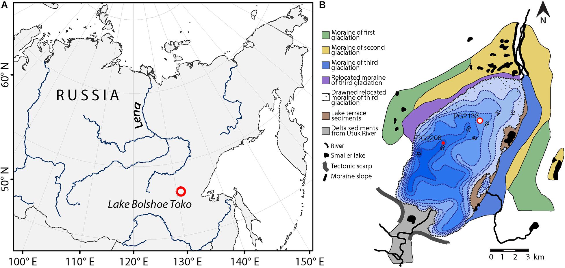
Figure 1. Study area. (A) Location of Lake Bolshoe Toko in southeastern Yakutia, Siberia. (B) Bathymetrical map with geological information and position of the sediment core PG2133 used for vegetation analyses in the northern part of the basin. Sediment core PG2208 was used to correlate Holocene ages between cores.

According to the data from the meteorological station, “Toko”, located ca. 10 km northeast of Lake Bolshoe Toko, mean annual air temperature is 11.2°C, ranging from −65°C in January to +34°C in July. Annual precipitation varies from 276 to 579 mm (Konstantinov, 2000). However, measurements taken directly at the lake suggest the influence of cold water from the Stanovoy Range that might cause slightly lower summer temperatures and thick ice during winter at the site.

Soil cover in the study area is thin and contains large amounts of gravel. The formation of soil is very slow because of deep seasonal freezing, short summers, and permafrost (Shahgedanova, 2002). The lake area belongs to the Aldan Floristic Region (Kuznetsova et al., 2010). Northern taiga dominates the study area. Forests consist of Larix cajanderi and L. gmelinii often accompanied by Picea obovata, P. jezoensis, and Pinus sylvestris (Konstantinov, 2000; Kuznetsova et al., 2010). The bedrock composition has an important influence on the vegetation: larch (Larix) and pine (Pinus) forest with a moss and lichen cover are especially common on the acidic metamorphic rocks, while in riparian areas small birch forests often form a belt around the mixed forest (Kuznetsova et al., 2010).

Fieldwork and Subsampling

Fieldwork was carried out by a German-Russian expedition in spring 2013. Sediment cores were recovered using a UWITEC piston coring system operated from the ice in the northern and central part of the lake (Figure 1B). This study is based on sediment core PG2133. The ice thickness was about 1 m and the measured water depth at this sampling point (56°04.582′N, 130°54.948′E) was 26 m. The 375 cm core was then cut into 1 m long pieces, transported unfrozen in plastic tubes to the laboratories of the Alfred Wegener Institute for Polar and Marine Research in Potsdam, Germany and stored there at 4°C until the subsampling for pollen and DNA analysis.

In December 2013 the core segments were cut into two halves. One was stored as an archive at 4°C and the other was scanned to correlate any overlaps. The opening and subsampling of the half-core for sedaDNA analysis was performed in the climate chamber of the Helmholtz Center Potsdam - German Research Center for Geosciences (GFZ) at 10°C, where no molecular genetic studies take place to prevent contamination with modern DNA. All surfaces in the climate chamber were cleaned with DNA Exitus Plus^TM (VWR, Germany) and demineralized water before working on the core. The sampling tools such as knives, scalpels, and their holders were cleaned before the taking of each sample following the recommendations of Champlot et al. (2010).

About 3 mm of each sample slice that was in touch with the plastic tube or the thin foil that covered the half-core was removed using a sterile scalpel as these parts cannot be considered sterile (Parducci et al., 2017). The samples for analysis were taken with the aid of 5 ml disposable syringes, in which the anterior cap had previously been cut off. A DNA sample was taken every two cm, giving 188 DNA samples over the 375 cm core length. In addition, 188 pollen samples were collected. The collected DNA samples were then stored at −20°C.

Core Splicing and Dating

The studied sediment core PG2133 was retrieved from the lake bottom as overlapping parts including a short core (PG2133-4) by gravity coring for undisturbed surface layers and two overlapping long-cores (PG2133-2, PG2133-3). The overlapping parts were spliced into one composite record by correlation of sediment layers using elemental (Zr) composition. We used geochemical variability in the stratigraphy validated by radiocarbon values to correlate the upper part of this core with the parallel core from the deeper central location PG2208 (Figure 1B). The higher resolution and more reliably dated Holocene part from PG2208 provides a precise delimitation of the Pleistocene-Holocene transition in core PG2133 (Figure 2). The transfer of the age-depth relation from PG2208 onto PG2133 younger than the last reliable tie-point (8400-8440 14C yrs BP, see Supplementary Table 1) is based on the assumption that sedimentation rates at both coring sites after the Late Holocene were stable until today and minor changes would have affected both coring sites in a similar direction.

FIGURE 2

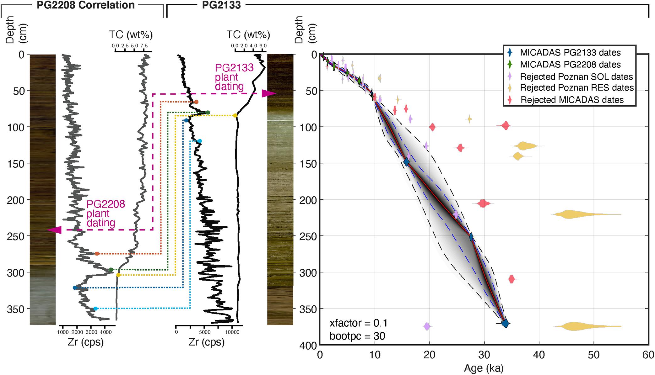
Figure 2. Age-depth model based on 22 radiocarbon dated samples from sediment cores PG2133, PG2208, and two surface samples (PG2112, PG2119) from Lake Bolshoe Toko, southeastern Yakutia, Siberia. Age-depth model created with the MATLAB software package ‘Undatable’ (Lougheed and Obrochta, 2019) and the IntCal20 calibration curve (Reimer et al., 2020). Modeled ages are expressed as calibrated thousand years (ka) before present. The Holocene part was correlated between sediment core PG2208, retrieved from the deeper central part of the lake, and sediment core PG2133. Correlation was performed using Zr values from XRF core scanner data shown as counts per seconds (cps) and the concentrations of total carbon (wt%). The purple arrows indicate the position of plant remains in photographs of the sediment cores, dated to similar ages found at different depths of both cores. Dashed lines indicate tie points between cores used to report age information from the higher resolution Holocene part from core PG2208 onto PG2133 used in this study.

Accelerator Mass Spectrometry (AMS) radiocarbon analysis was carried out on bulk sediment material and woody plant remains at the Poznań Radiocarbon Laboratory, Poland, and at the MICADAS radiocarbon laboratory, AWI Bremerhaven. In total 49 samples were measured for radiocarbon including 24 samples from PG2133, 23 samples from PG2208, and two surface samples in proximity of these cores. All samples were bulk sediment samples, with the exception of two plant remains of the same age, one from each core used for correlation between 242.5 cm (PG2208) and 53.5 cm (PG2133). The results from Poznań and MICADAS labs are partly inconsistent due to different pretreatment methods. Poznań either measured the humic acid fraction (“SOL”, soluble in NaOH) and/or the humin fraction (“RES”, residual, i.e., alkali-insoluble fraction). MICADAS measured following their standard acid treatment method outlined in detail in Vyse et al. (2020). Due to the large deviation between SOL and RES samples of the bulk samples from Poznań compared to a better down-core consistency of MICADAS samples, we used MICADAS bulk samples and the dating of plant remains from Poznań for age-depth modeling. We excluded samples that are influenced by old organic carbon (Biskaborn et al., 2019a) detected by deviation from an approximate linear relationship. We used the surface samples PG2112 for reservoir correction (1203 yr) of PG2133 and PG2119 for reservoir correction (762 yr) of PG2208 (Supplementary Table 1). For modeling we used the open-source MATLAB software package ‘Undatable’ (Lougheed and Obrochta, 2019), version 1.3.1 with the settings: nsim = 105, bootpc = 30, xfactor = 0.1 and the IntCal20 calibration curve (Reimer et al., 2020).

Sediment-Geochemical Analyses

To gain information on the organic matter chemistry we analyzed 75 samples for total carbon (TC) and nitrogen (TN), and 69 samples for total organic carbon (TOC). Freeze-dried and milled sample material was measured in tin boats using an elemental analyzer (Elementar Vario EL III) for TC and TN. For TOC, where enough material was left, material from the same sample boxes were placed into small crucibles and measured with a Vario MAX C analyzer. The per cent by weight of TOC and TN were used to calculate the TOC/TN_atomic ratio following Meyers and Teranes (2002). However, below 80 cm in core PG2133, TN contents were less than 0.1 wt% and could not be detected by the device. Therefore, for these samples with TN <0.1, we used 0.09 as an estimate to calculate the TOC/TN_atomic ratios, marking the samples as “uncertain” in the down-core plot (Figure 3).

FIGURE 3

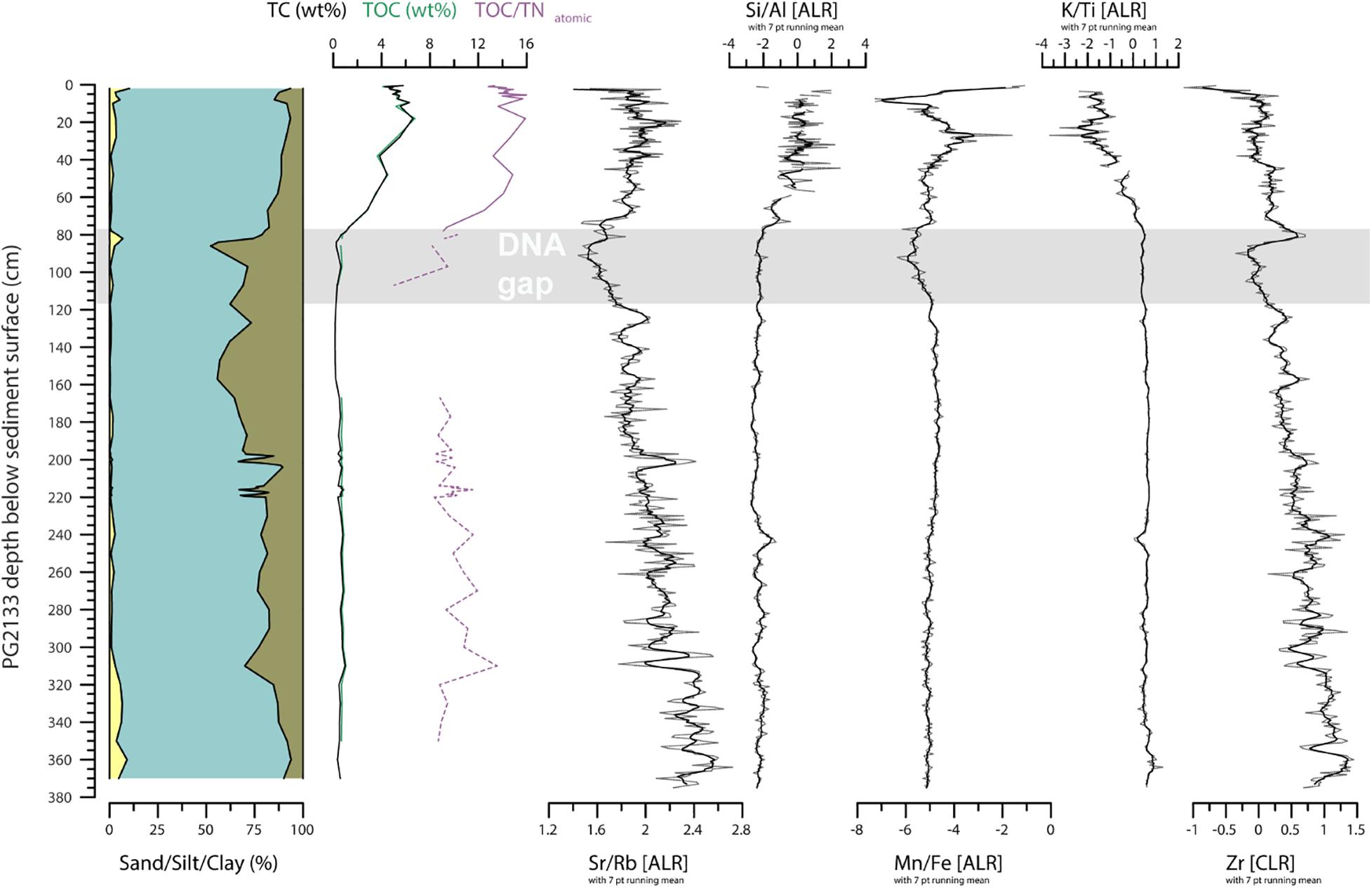
Figure 3. Sedimentary and geochemical composition of sediment core PG2133 including grain-size distribution, carbon concentrations, and XRF elements. Sand, silt, and clay proportions are reported over the entire PG2133 core. Total carbon (TC), total organic carbon (TOC), and the ratio of TOC to nitrogen (TOC/TN_atomic) are reported to indicate input of terrestrial plant material relative to aquatic algae (Meyers, 2003; Biskaborn et al., 2012). The Strontium (Sr) over Rubidium (Rb) ratio and Zirconium (Zr) indicate relative detrital input related to coarse grain size (Biskaborn et al., 2013). The Silicon (Si) over Aluminum (Al) ratio indicates the occurrence of diatom valves (Vyse et al., 2020). The Manganese (Mn) and Iron (Fe) ratio indicate redox dynamics associated with bottom water oxygenation (Melles et al., 2012; Naeher et al., 2013), which with the Potassium (K) over Titanium (Ti) ratio, provides information on physical versus chemical weathering in the catchment (Vyse et al., 2020). Shaded area indicates a gap in the DNA data.

Sediment grain-size distribution was generated using a laser to determine the grain sizes of 65 samples. We removed organic compounds by soaking samples in hydrogen peroxide (3%) for 5 weeks, while the pH was kept neutral using drops of ammonia and acetic acid 3 times per week. After washing by adding water, centrifuging, and decanting, we added sodium pyrophosphate to homogenize samples in an overhead shaker. Particle size was measured by laser diffractometry using a Malvern Mastersizer 3000. We used averaged values after a minimum of 9 measurements. Clay, silt, sand, and gravel fractions were calculated as the sums of the volume percentages using boundaries <2 μm, 2–63 μm, 63 μm–2 mm, and 2–63 mm, respectively.

To gain information on the inorganic elemental composition of the sediments, non-destructive X-ray fluorescence was performed on one half of each core section including overlapping parts using an AVAATECH XRF core scanner at AWI in Bremerhaven. Light elements including Al, Si, K, Ti, Mn, and Fe, were measured at 10 kV using a Rh X-ray tube, 1.2 mA, 12 s count time, and no filter. Heavier elements including Rb, Sr, and Zr, were measured at 30 kV using a Rh X-ray tube, 1.5 mA, 15 s count time, and a thick Pd-Filter. To account for data compositional effects, scanning results originally expressed in counts per second (cps) were additive log-ratio (ALR) and centered log-ratio transformed (Weltje and Tjallingii, 2008) for ratios and single elements, respectively (Figure 3). We used original cps values to correlate between cores PG2133 and PG2208 to prevent differences in XRF device settings between cores influencing other elements included in the CLR transformation and thus bias a core-to-core correlation.

Pollen Analysis

Sixty-seven samples of 3 g (wet weight) were selected for pollen analysis. Standard preparation including KOH, HCl treatment, boiling with HF, and acetolysis was used to concentrate palynomorphs (Faegri and Iversen, 1989). A Lycopodium spore tablet (batch no. 1031; n = 20,848 ± 1460) was added to each sample to calculate pollen concentration (Stockmarr, 1971). Palynomorphs were identified using a light microscope (Zeiss Axioskop 2) under 400–600 × magnification. At least 300 terrestrial plant pollen grains were counted in each sample. Pollen atlases (Sokolovskaya, 1958; Kupriyanova and Alyoshina, 1972, 1978; Moore et al., 1991; Beug, 2004; Savelieva et al., 2013) and pollen reference collections at the Arctic and Antarctic Research Institute (Saint Petersburg) and the Alfred Wegener Institute were used for taxonomic identification of pollen and spores. Non-pollen palynomorphs (NPP) were determined according to van Geel (2001); van Geel et al. (1983), and van Geel and Aptroot (2006). Freshwater algae were determined using Jankovská and Komárek (2000) and Komárek and Jankovska (2003). Only the terrestrial pollen data are presented here, however, all data are archived in DRYAD at “10.5061/dryad.34tmpg4gz”.

Molecular Genetic Preparation

DNA isolation and polymerase chain reaction (PCR) setup were performed in the paleogenetic laboratory of the Alfred-Wegener-Institute Helmholtz Center for Polar and Marine Research in Potsdam, Germany. This lab is dedicated to ancient DNA isolation and PCR setup and is located in a building devoid of any molecular genetic lab work. The lab is cleaned frequently and subjected to nightly UV-irradiation. All laboratory work was performed in a UVC/T-M-AR DNA/RNA cleaner-box (BIOSAN, Latvia). DNA isolations and PCR setups were performed on different days using dedicated sets of pipettes and equipment. Further precautions to reduce contamination included UV-irradiation of 10× buffer, BSA, MgSO4, and DEPC-treated water for 10 min in a UV crosslinker in thin-walled PCR reaction tubes (recommendations of Champlot et al., 2010).

In total, 54 samples were selected for DNA extraction ranging from 1 to 374 cm depth. Six separate extractions were performed, each with nine samples and one control (blank). Total DNA was isolated from approximately 3 g of sample material using the PowerMax^® Soil DNA Isolation Kit (Mo Bio Laboratories, Inc., USA) added to 1.2 ml of C1 buffer (PowerMax^® Soil DNA Isolation Kit, Mo Bio Laboratories, Inc., USA), 0.4 ml of 2 mg/mL Proteinase K (protK, VWR International, Germany) and 0.5 ml of 1 M dithiothreitol (DTT, VWR International, Germany). This mixture was homogenized for 10 minutes on a vibratory mixer (VortexGenie2, Mo Bio Laboratories, USA) and incubated overnight at 56°C while rotating. All subsequent steps were performed according to the instructions of the manufacturer Qiagen, except for the last step in which 800 μL elution buffer (C6 buffer) was applied to the filter membrane, incubated for 10 minutes at room temperature, and then centrifuged for 3 minutes at 2500x g. This step was performed twice ending up with a final volume of 1.6 ml.

The PCR reactions were performed using the trnL g and h primers (Taberlet et al., 2007). Both primers were modified on the 5′ end by unique 8 bp tags which varied from each other in at least five base pairs to distinguish samples after sequencing (Binladen et al., 2007) and were additionally elongated by NNN tagging to improve cluster detection on the sequencing platform (De Barba et al., 2014). The PCR reactions contained 1.25U Platinum^® Taq High Fidelity DNA Polymerase (Invitrogen, USA), 1× HiFi buffer, 2 m MMgSO4, 0.25 mM mixed dNTPs, 0.8 mg Bovine Serum Albumin (VWR, Germany), 0.2 mM of each primer, and 3 μL DNA in a final volume of 25 μL. PCRs were carried out in a Professional Basic Thermocycler (Biometra, Germany) with initial denaturation at 94°C for 5 min, followed by 50 cycles of 94°C for 30 s, 50°C for 30 s, 68°C for 30 s, and a final extension at 72°C for 10 min. The extraction blank and one no template control (NTC) was included in each PCR to identify possible contamination during extraction and PCR set-up. For each extraction sample, two PCR replicates with different primers were performed. PCR success was checked with gel-electrophoresis on 2% agarose (Carl Roth GmbH & Co. KG, Germany) gels were used. The PCR products were purified using the MinElute PCR Purification Kit (Qiagen, Germany), following the manufacturer’s recommendations. Elution was carried out twice with the elution buffer to a final volume of 40 μL. The DNA concentrations were estimated with the dsDNA BR Assay and the Qubit 2.0 fluorometer (Invitrogen, USA) using 1 μL of the purified amplifications. To avoid bias based on differences in DNA concentration between samples, all replicates (except for samples 20, 86, and 106 where only one sample was used) were pooled in equimolar concentrations. All extraction blanks and NTCs (9 extraction blanks and 11 PCR NTCs) were included in the sequencing run, using a standardized volume of 10 μL, even though they were negative in the PCRs. The sequencing results of extraction blanks and PCR controls are reported in the Supplement. Fasteris SA sequencing service (Switzerland) performed the paired-end sequencing on one-tenth of a full lane of the Illumina HiSeq platform (2 × 125 bp).

Processing of SedaDNA Data

Filtering, sorting, and taxonomic assignments of the sequences were performed with OBITools (Boyer et al., 2015). Using the function illuminapairedend, forward and reverse reads were aligned to produce merged sequences. Based on exact matches to their tag-combination, they were assigned to their samples using ngsfilter. Sequences shorter than 10bp were excluded with obigrep and duplicated sequences were merged with obiuniq while keeping the information to which sample the sequences originally belonged. Sequences with fewer than 10 read counts were excluded from the dataset as they are probably artifacts. Obiclean was used to exclude sequence variants probably attributable to PCR or sequencing errors (Boyer et al., 2015). Two reference databases were used for taxonomic assignments (Epp et al., 2015). The first one, ArctBorBryo, is based on the quality-checked and curated Arctic and Boreal vascular plant and bryophyte reference libraries (Sønstebø et al., 2010; Willerslev et al., 2014; Soininen et al., 2015). The second is based on the EMBL Nucleotide Database standard sequence release 133 (Kanz et al., 2005¹). The sequences were assigned to taxon names based on sequence similarity to each of the reference databases using the function ecotag.

The database that gave the best identity was selected with a priority for ArctBorBryo database if both gave the same identity, as it is a more specific database for boreal species. Only sequences assigned with a best identity of 100% and that are present in at least two replicates or samples are used in this study. The sequence types assigned with a 100% value to an unknown family level were removed. Taxa and sequences from the extraction and PCR NTCs were checked and removed from the dataset if their relative proportion in the controls was greater than 0.5%. The PCR replicates were merged to work with 54 samples. Sequences assigned to the same taxon were merged and those sequences that appeared fewer than 10 times in a sample were removed from it. Sequences were assigned to aquatic, bryophyte, or terrestrial taxa and only the terrestrial ones were selected for this study. Samples at 78, 82, 86, and 106 cm were represented by no terrestrial plant reads after these filtering steps.

Before proceeding to the data analysis, a rarefaction analysis to compare the richness at a similar level of sampling effort was performed based on the minimum number of observed sequence counts (n = 4119 (sample at 96 cm); highest sequence count is n = 329924, from 366 cm).

Statistical Analysis and Visualization

The paleogenetic and palynological datasets are archived in DRYAD at “10.5061/dryad.34tmpg4gz”.

Composition Analysis

To allow visual comparison of the different records and changes of abundance through time, percentage bar plots of taxa were produced for pollen and sedaDNA datasets using the strat.plot function from the rioja R-package (Juggins, 2019). In addition, the summed proportions of tree, shrub, or herb taxa for sedaDNA or tree/shrub and herb taxa for pollen were plotted. A constrained hierarchical clustering approach (CONISS) (Grimm, 1987) was performed with clusters constrained by depth/ages using vegdist from the vegan R-package (Oksanen et al., 2019) and chclust from the rioja R-package. The samples with 0 read counts were excluded from this analysis. Zones were determined by the broken-stick model (MacArthur, 1957; Bennett, 1996) using bstick from the vegan R-package.

A principal component analysis (PCA) was run on the double square-root transformed relative proportions for sedaDNA and square-root transformed pollen data using the rda function in the vegan R-package (Oksanen et al., 2019) to portray the major structure in the multivariate dataset. For the sedaDNA record, samples with 3 or fewer taxa detected were removed before performing the PCA as those samples might not be representative of the vegetation composition. Principle component 1 and 2 (PC1 and PC2) axes scores were extracted and visualized in biplots. For better visibility, only the name of terrestrial taxa that explain most variance are printed.

To allow direct comparison of the records, pollen and sedaDNA taxa were harmonized to the lowest common taxonomic level (e.g., Ericaceae taxa were transformed to Ericales). PCAs were rerun for each record including only those samples that are present in both datasets. To compare the fit between sample and species scores of the first PCA axes for pollen and sedaDNA, Procrustes rotation analyses were performed (Peres-Neto and Jackson, 2001) and the significance of similarity between the datasets was tested by PROTEST (Jackson, 1995).

Richness Analysis

Taxa richness is here defined as the number of different taxa counted per sample. It was measured for each depth/age from the rarefied DNA results with the ChaoRichness command from the iNEXT R-package (Hsieh et al., 2016). To test the significance of the difference in the average taxa richness between different zones determined by the broken-stick model, a non-parametric Wilcoxon rank sum test was performed.

After resampling the two most common families of the DNAZ I to 1000 reads (Saxifragaceae and Asteraceae), the same test was performed to compare the taxa richness within those families and their impact on the DNAZ I richness.

Statistical analyses and age-depth modeling were performed in R v. 3.6.1 (R Core Team, 2019). Statistics were mainly performed using the packages “vegan” version 2.5-6 (Oksanen et al., 2019), “rioja” version 0.9.21 (Juggins, 2019), “iNEXT” version 2.0.20 (Hsieh et al., 2016) and “analog” version 0.17-3 (Simpson, 2007; Simpson and Oksanen, 2016).

Results

Age Model

Modeled dates for PG2133 are expressed as calibrated years before present relative to 1950 CE (cal. yr BP). The Pleistocene-Holocene boundary detected by the main lithological transition found at ca. 80–82 cm revealed an age between 10,765 and 11,924 cal. yr BP (sigma 2 range). The maximum modeled age in the core is 33,478–34,126 cal. yr BP at 370.5 cm composite depth below sediment surface (Figure 2). Accordingly, the mean sedimentation rate during the Holocene was 0.007 cm a^–1, and 0.01 cm a^–1 during the Pleistocene part of the core. Differences in sedimentation rates between distant sediment cores shown in Figure 2 is common in large lakes (Jenny et al., 2014). The drop in sedimentation rate after the deglaciation period is likely a result of decreased clastic input from the catchment as indicated by decreasing Zr (Biskaborn et al., 2019a). The mean sigma 2 uncertainty ranges in the Holocene and Pleistocene are estimated as 517.6 and 2378.8 yr, respectively. In this study, for simplicity, we use mean values to estimate the timing of transitions between pollen zones.

Sediment-Geochemical Core Composition

The Pleistocene section below 80 cm in sediment core PG2133 reveals organic-poor clayey silt (Figure 3). Here the mean value for gravel, sand, silt, and clay is <0.01, 1.8, 73.3, and 24.9%, respectively. The TC and TOC contents are 0.6 and 0.7%, respectively, with a negligible difference resulting from measurements with different devices (TC-TOC difference over the whole core is mean -0.06 wt%, min. -0.48 wt%, and max. 0.35 wt%). The TN/TOC_atomic ratios remain low at around 9.6 (note: this section is based on estimated TN values because the nitrogen values remained under the detection limit, see Materials and Methods section). Zr (both cps values, Figure 2 and CLR values, Figure 3) has generally higher values in the Pleistocene section below 80 cm, with a strong peak that correlates to a small sand peak in the transition zone between 77 and 83 cm. K/Ti has uniformly high values in the Pleistocene, whereas Sr/Rb fluctuates with highest values at the bottom of the core and lowest values at the Pleistocene–Holocene transition. Si/Al is low with only minor excursions in the Pleistocene. Mn/Fe is also low but slightly decreases at 113 cm toward the top of the core.

In the Holocene core section, the grain-size composition is slightly less clayey, but still dominated by silt (mean values: sand 2.9, silt 84.1, clay 13.1%) with increased carbon content (mean value: TC 4.5 wt%) and TOC/TN_atomic ratios (mean value: 13.7), which is within the ranges reported from Bolshoe Toko short cores covering the past few decades (Biskaborn et al., 2021). Sr/Rb, Si/Al, and Mn/Fe increase in the early Holocene, whereas K/Ti decreases. Between ca. 30 cm and the top of the core Mn/Fe decreases after a maximum, and K/Ti increases after a minimum. Close to the sediment surface the values of Sr/Rb and Mn/Fe exhibit strong fluctuations, which could reflect the effect of higher water content in the unconsolidated surface sediments.

Pollen Stratigraphy

A total of 111 different terrestrial pollen, spores, and NPP taxa were identified in the 67 samples. Only terrestrial pollen taxa are presented on the pollen diagram (Figure 4) for a direct comparison with the sedaDNA diagram (Figure 5). The entire pollen dataset is presented in Supplementary Figure 1. The pollen assemblages can be subdivided into 3 main pollen zones (PZ) according to CONISS analysis.

FIGURE 4

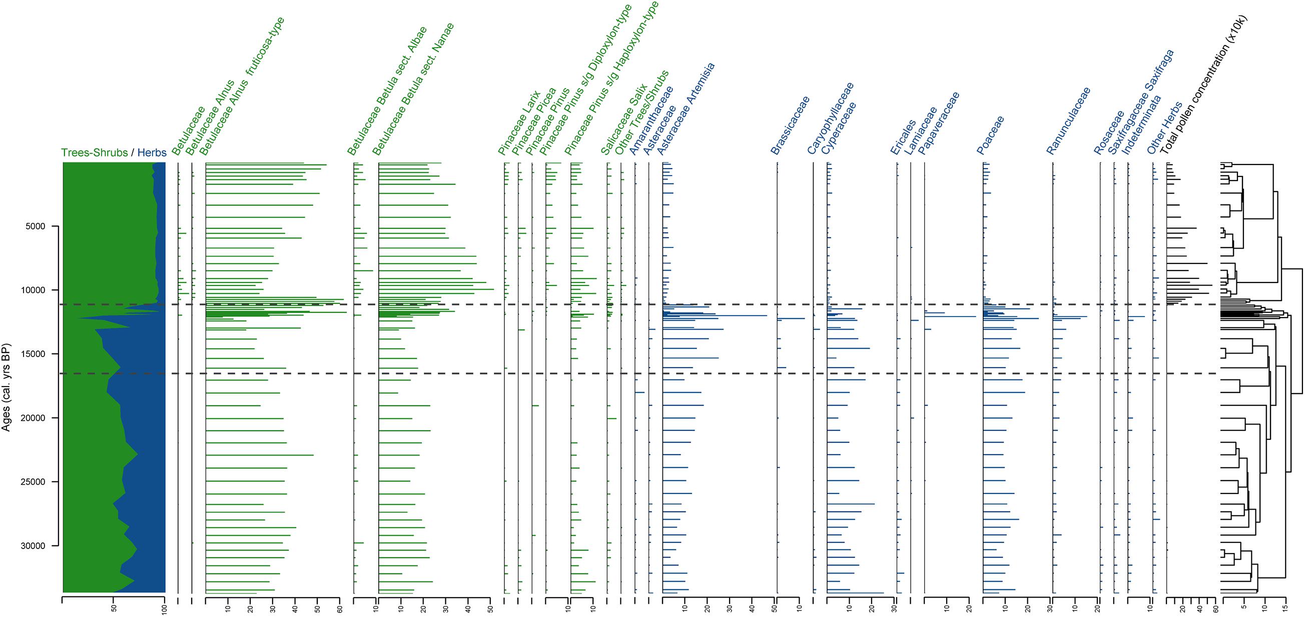
Figure 4. Stratigraphic plot of terrestrial pollen with relative percentages of the taxa in each sample as horizontal bars, ratio of tree/shrub taxa vs herb taxa, and CONISS dendrogram. The taxa are sorted at genus level for trees and shrubs and at family level for herbs. Three pollen zones (PZ) are shown derived from the CONISS analysis. Samples from sediment core PG2133 are plotted against calibrated ages given in cal yr BP.

FIGURE 5

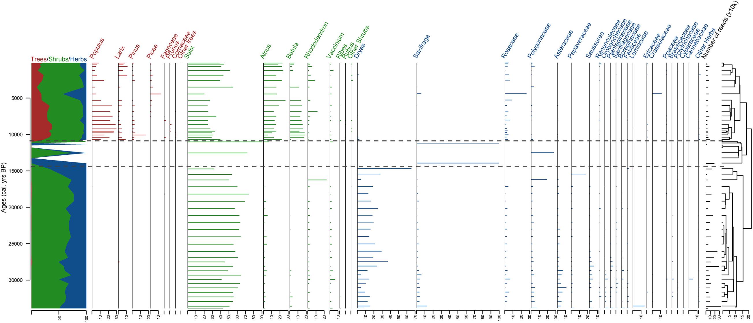
Figure 5. Stratigraphic plot of terrestrial sedaDNA with relative percentages of the taxa in each sample as horizontal bars, ratio of tree/shrub taxa vs herb taxa, and CONISS dendrogram. The taxa are sorted at genus level for trees and shrubs and at family level for herbs. Three sedaDNA zones (DNAZ) are shown, derived from the CONISS analysis. Calibrated ages from the age–depth model are given in calendar years before present (cal yr BP).

PZ I (ca. 374–96 cm, >33,800–12,474 cal yr BP is characterized by rather low pollen concentrations varying between 486 and 19,795 pollen grains per gram (gr g^–1) with 6,027 on average. Tree and shrub pollen average 55% (varying from 30.3 to 72.7%). The most common shrub pollen taxa are Alnus fruticosa-type (31.8% on average) and Betula sect. Nanae (16.8% on average). Herb pollen taxa (45% on average, varying from 27.3 to 69.3%) are mostly represented by Artemisia (12.3% on average), Poaceae (11.9% on average), and Cyperaceae (11.4% on average).

Pollen concentration in PZ II (ca. 94–80 cm, 12,329–11,268 cal yr BP) is even lower than in PZ I (2,479 gr g^–1 on average, varying from 201 to 9,677 gr g–1). Tree and shrub pollen taxa dominate the spectra of most samples (up to 93.6%, on average 61%), while herb taxa vary from 6.4 to 87.5% (on average 39%). Alnus fruticosa-type (35.3% on average) and Betula sect. Nanae (20.5% on average) are still the most dominant pollen taxa. The most represented herb pollen taxa are Artemisia (15.2% on average) and Poaceae (10.2%), with Cyperaceae (4.4%), Papaveraceae (3%), and Ranunculaceae (3%) also represented.

Pollen concentration drastically increases (up to 558,726 gr g^–1, on average 244,074 gr g^–1) at the beginning of PZ III (ca. 78–0 cm, 11,112 cal yr BP to present), but gradually decreases after 24 cm (4,373 cal yr BP). Tree and shrub pollen taxa dominate the spectra (on average 90%). The most common shrub pollen taxa are Alnus fruticosa-type (38.1% on average) and Betula sect. Nanae (33.8%). Alnus fruticosa-type percentages are highest between 78 and 72 cm (11,112 to 10,643 cal yr BP). Betula sect. Nanae pollen percentages increase around 72 cm (10,643 cal yr BP) and gradually decrease upward. More tree pollen taxa are also detected in this zone: Larix (1.3% on average), Pinus s/g Diploxylon-type (2.6%) and P. s/g Haploxylon-type (5.6%). The herb taxa are less numerous than in the lower PZs (9.9% on average, varying from 7.1 to 13.4%). They are dominated by Artemisia (3.2% on average), Poaceae (1.6%), and Cyperaceae (1.4%).

The first two axes of the PCA (Figure 6) explain 52.7% of the variance in the dataset, supporting the zonation of the broken-stick analysis. Samples from PZ I are mostly in the left-hand quadrants, represented mainly by Cyperaceae, Poaceae, and Artemisia. The samples from PZ II are spread across PC1 and intermix with samples from PZ I and PZ III. Samples from PZ III are mostly located in the right-hand quadrants and are represented by taxa such as Pinus s/g Haploxylon-type, Betula sect. Albae, Pinus s/g Diploxylon-type, Betula sect. Nanae, and Alnus fruticosa-type as well as Larix, Picea, and Salix.

FIGURE 6

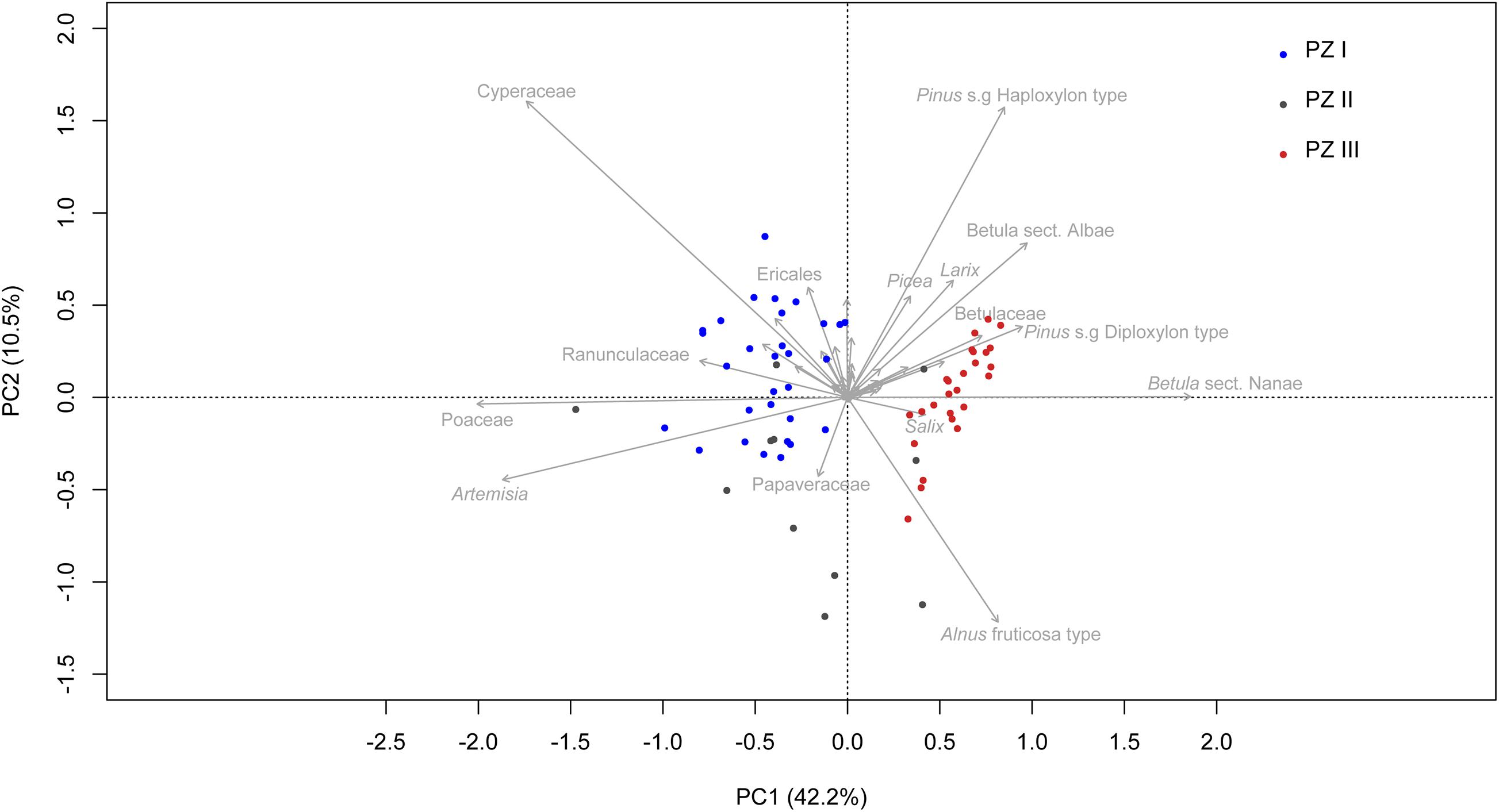
Figure 6. Principal component analysis (PCA) biplot of terrestrial pollen taxa. Only the names of the 15 taxa explaining the most variance are printed. Samples are colored according to their corresponding zone. The explained variances of the two principal components (PC1 & 2) are shown in brackets.

SedaDNA Composition

In total, 10,172,402 reads were assigned to 3,007 different sequences types with more than 10 counts. 5,364,355 were assigned with 100% identity to 322 sequence types. In total, 8 sequence types were present in the controls. There were three different sequence types with 274,319 (5.1% from total dataset) total reads in 3 of the 9 PCR NTCs and 6 sequence types with 904,427 (16.9% from total dataset) total reads in 6 of the 11 extraction blanks. Two sequence types assigned to Brassicaceae were removed from the dataset as all their reads were present in the controls; as was one sequence type assigned to Taxus baccata for which 91% of its reads were present in one NTC and the rest in only one other replicate. Five other sequence types (assigned to Bistorta vivipara, Salicaceae, Asteraceae, Saxifraga cernua, and Pinus) were kept for the analysis after examination. For Bistorta vivipara, 1 read was present in the controls, for Salicaceae, 7 reads (<0.001%) in 4 controls, and 1 read for Asteraceae and Saxifraga cernua. For Pinus, 388,820 and 1 reads (94%) were detected in 2 extraction blanks, but is also present in 35 other PCR replicates in coherent proportions with no link to the problematic extraction blanks. The sequence type assigned to Convallaria majalis with 14,702 reads was deleted from the dataset as it is a common contaminant and 9 sequence types not even assigned to the family level at best were removed for a total of 633 reads. Furthermore, 64 sequence types with a total of 9,258 reads that appear in only one PCR product were deleted. After the replicates were merged and those with the same assignment merged (54 samples), 181 taxa were detected with 4,159,565 reads in total and 4,157,784 reads when the taxa with fewer than 10 reads were deleted.

In total, 4,133,309 sequence counts were assigned to 153 terrestrial plant taxa across 50 samples: 82 to species level, 55 to genus level, and 16 only to family level at best. The most common families among the dataset that represent 90% of the reads are Salicaceae (52%), Rosaceae (13%), Betulaceae (12%), Saxifragaceae (6%), Ericaceae (4%), Pinaceae (3%), and Asteraceae (2%).

The terrestrial plant sedaDNA dataset can be divided into three zones according to the CONISS clustering and broken stick analysis (Figure 5). Because of the high number of taxa detected using DNA, tree and shrub taxa are plotted at the genus level and herbs at the family level. The detailed dataset is presented in Supplementary Figure 2.

DNAZ I (ca. 374–126 cm, >33,800–14,660 cal yr BP) with 26 samples approximately matches PZ I. This zone is represented mostly by shrub taxa (from 32.3 to 76.6% with 62.2% on average) with Salix (56.2% on average) dominant. Herb taxa also have high proportions (23 to 67.7% with 37.6% on average) with Dryas (18.3% on average) and other Rosaceae (2% on average) as well as Asteraceae (4.4%) represented by Artemisia and Saussurea. Tree taxa are present in DNAZ I at low percentages (0 to 1.6% with 0.2% on average).

DNAZ II (ca. 116–76 cm, 13,901–10,956 cal yr BP) is represented by 8 samples: 4 samples are represented by very few reads and 4 had no sequence types at all but were added anyway. Only a few taxa are found in the zone: Salix and Polygonaceae at 96 cm (12,474 cal yr BP), 2 taxa from Saxifragaceae in the samples at 116 and 80 cm (13,901 and 11,268 cal yr BP, respectively), and Alnus, Salix, and Vaccinium in the sample at 76 cm (10,956cal yr BP). The zone has a high proportion of herbs (up to 100% with 56.8% on average), with Polygonaceae (6.9% on average) and Saxifraga (49.9%) as the most abundant taxa. Shrub taxa are also found (43.2% on average, ranging from 0 to 100%) mostly represented by Salix (40.6% on average), but not a single tree taxon.

The uppermost zone, DNAZ III (ca. 72–0 cm, 10,643 cal yr BP to present) has 20 samples and has more tree taxa than the lower zones (24.9% on average, ranging from 9.3 to 37.5%), mostly Populus (15.7%), Larix (4.3%), Pinus (2.6%), and Picea (1.5%). Shrubs are also highly represented (38.8 to 86.1% with 65.3% on average) with 34.1% Salix on average, 16.8% Alnus, 9.9% Betula, and 2.5% Rhododendron. Some herb taxa (3.7 to 43.3% with 9.7% on average) are also found. The most represented herb taxa are Rosaceae (4.7% on average), Polygonaceae (1%), Crassulaceae (0.6%), Ranunculaceae (0.6%), and Saxifragaceae (0.6%). In DNAZ III, notable variations can be seen and this zone can be divided into two subzones. In the lower part, DNAZ IIIa (72–28 cm, 10,643–5,242 cal yr BP), trees are abundant (30.6% on average) with a high proportion of Populus (21.9%). At 24 cm (4,373 cal yr BP), a peak in Picea (13%) is observed as well as a peak in Rosaceae (26.2%), Crassulaceae (11.3%), and Saxifraga (4.6%). In the upper part, DNAZ IIIb (20–1 cm, 3,432–111 cal yr BP), fewer tree taxa (16.2% on average) are present, with less Populus (6.7%) but more Larix (up to 6.4% vs 3.5% in DNAZ IIIa) and more shrubs (74.9%) such as Salicaceae (44.6%). More Alnus (20% vs 15% in DNAZ IIIa) and less Betula (4.1% vs 14.1% in DNAZ IIIa) are also noticeable.

The first two axes of the PCA (Figure 7) explain 53.7% of the variance in the dataset, supporting the differentiation between DNAZ I and DNAZ III from the broken-stick analysis. Samples from DNAZ I are mostly in the right-hand quadrants and are mainly represented by Dryas, Asteraceae, Plantaginaceae, Boraginaceae, and Papaveraceae. The samples from DNAZ III are mostly located on the left-hand quadrants and are represented by taxa such as Betula, Alnus, Larix, Pinus, Picea, and Populus.

FIGURE 7

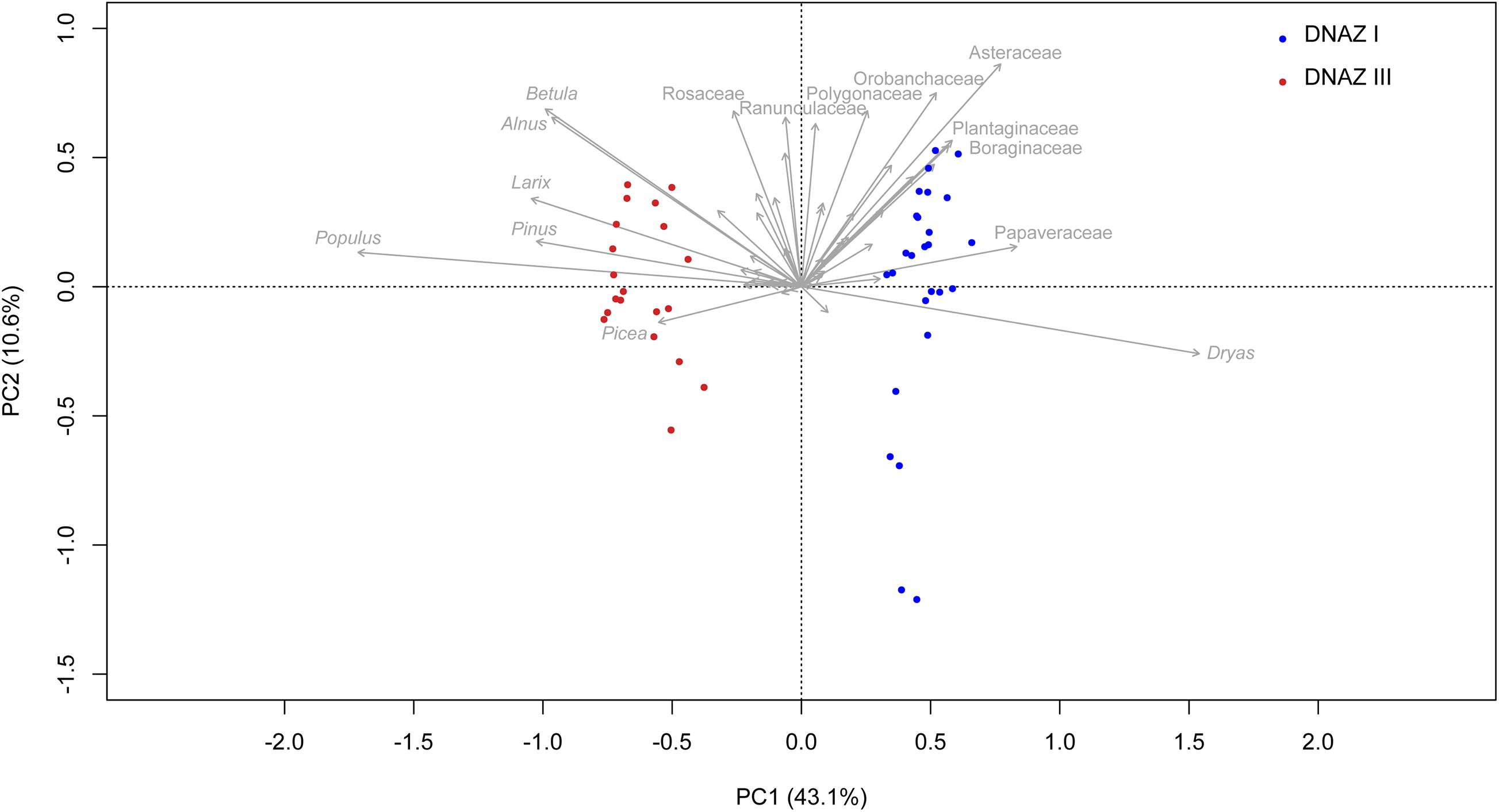
Figure 7. Principal component analysis (PCA) biplot of sedaDNA terrestrial taxa. Only the names of the 15 taxa explaining the most variance are printed. Samples are colored according to their corresponding zone. The explained variances of the two principal components (PC1 and PC2) are shown in brackets.

Comparison Between Pollen and SedaDNA

Results of the Procrustes rotation analyses and PROTEST (Table 1) indicate significant concordance between the pollen and sedaDNA PCA sample scores (m¹² = 0.536, p = 0.001) as well as taxa (m¹² = 0.7879, p = 0.001). Age residuals between 22,981 and 10,330 cal yr BP are mostly above average (Figure 8A) showing weak similarity for this time between both proxies. The sample dated to 33,815 cal yr BP has the lowest similarity between the sedaDNA and pollen datasets. The sample dated to 4,373 cal yr BP is similarly weak. Taxa residuals of Salix, Populus, and Dryas have the highest above-average values implying very weak similarity for these taxa between the pollen and sedaDNA datasets (Figure 8B). Furthermore, Artemisia, Alnus, Cyperaceae, Ericales, Papaveraceae, Larix, Polygonaceae, Rosaceae, and Saxifragaceae are also well above average and therefore dissimilar between both proxies.

TABLE 1

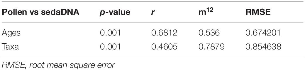
Table 1. Results of Procrustes and PROTEST analyses indicate significant fit among all pairwise comparisons of datasets obtained by pollen and sedaDNA analyses.

FIGURE 8

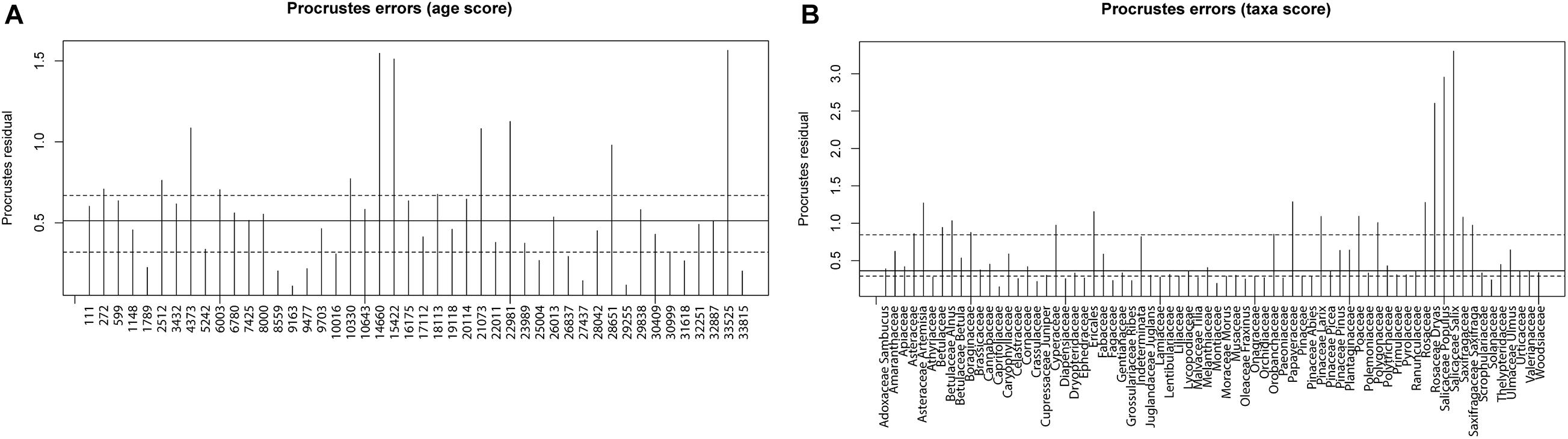
Figure 8. Procrustes residuals plots. (A) Procrustes residuals plot of the comparison of principal component analysis (PCA) depth/age scores of sedaDNA and pollen data presented as residuals of depth/age scores reflecting dissimilarity between the tested datasets. Dashed lines are the first and third quartiles, while the solid line is the second quartile. (B) Procrustes residuals plot of the comparison of PCA taxa scores of sedaDNA and pollen data presented as residuals of taxa scores reflecting dissimilarity between the tested datasets. Dashed lines are the first and third quartiles, while the solid line is the second quartile.

Taxa Richness Investigation

The test of significance of the difference in the average taxa richness focused on the difference between DNA Zone I and DNA Zone III. DNAZ II was excluded from this analysis for the same reasons as explained before. Furthermore, the three most recent samples from DNAZ I that make the transition to DNAZ II were also removed from this analysis and the visualization.

DNAZ I has on average 38 taxa ranging from 10 to 54 (Figure 9), while DNAZ III has 29 taxa on average with a range of 14 to 46. Taxa richness is significantly higher in DNAZ I (Wilcoxon rank sum test with continuity correction, W = 353, p = 0.001).

FIGURE 9

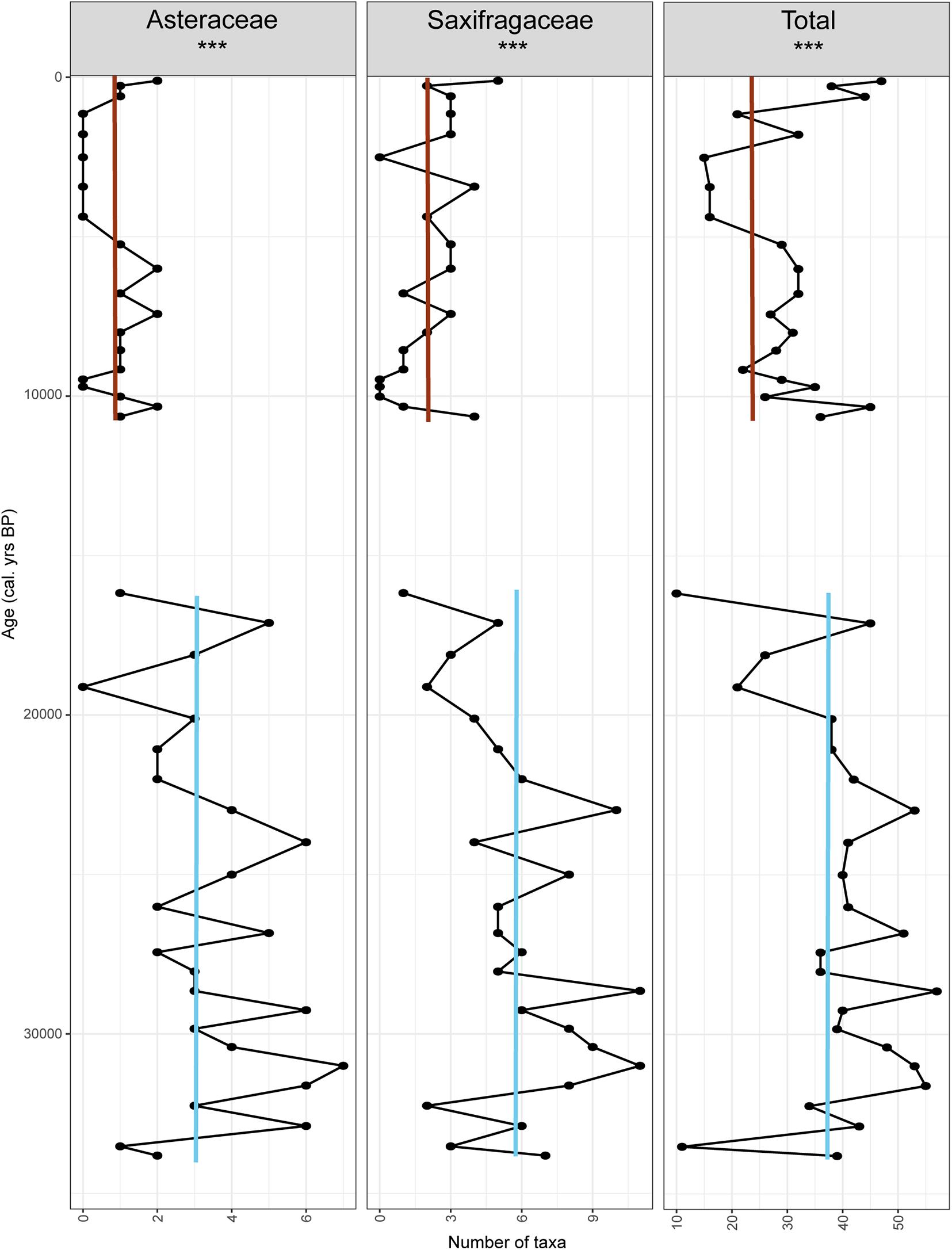
Figure 9. Richness count (total and within the most represented families). Red lines indicate average values in the Holocene interglacial while blue lines indicate the average during the last glacial period.

The taxa richness within the two most represented families detected in DNAZ I was also investigated (Figure 9). For Asteraceae, taxa richness is significantly higher in DNAZ I (3 on average) than in DNAZ III (0.8 on average, W = 435, p < 0.001). The same is found for Saxifragaceae with an average of 4.9 taxa in DNAZ I and 2 in DNAZ III (W = 421, p < 0.001).

Discussion

Proxy Validation

While the age-depth model has wide confidence intervals for the lower part of the core, the Holocene part of the model is more precise. According to the age-depth model, the bottom part of the core is dated to a mean extrapolated age of about 35,000 cal yr BP, and the sediments with the highest herb percentages thus accumulated between ca 22,000 and 12,500 cal yr BP, during the Marine Isotope Stage (MIS) 2, known for its harsh climate and herb-dominated vegetation. Therefore, we consider that the lower part can be interpreted at a rough MIS timescale while millennial-scale variation can be inferred in the Holocene interglacial part.

In our pollen assemblages, Alnus fruticosa-type, Betula sect. Nanae, Artemisia, and Poaceae are present at high percentages (Figure 3). All these taxa are known to be high pollen producers with good dispersal abilities (Niemeyer et al., 2015) and mainly originate from the regional vegetation. As these biases are rather similar in all pollen records, pollen data from different locations are principally comparable and relative abundances of major plant taxa can be reconstructed. Accordingly, we assume that our pollen data are also useful to infer major regional-scale vegetation composition changes. On the one hand, typically diverse herb families are mostly underrepresented (e.g., Rosaceae) but on the other hand, our pollen record contains pollen likely originating from long-distance sources (e.g., Pinus during the glacial period). Furthermore, many pollen types can only be identified to family level (e.g., Poaceae, Cyperaceae, Brassicaceae). Therefore, we consider our pollen record as not so suitable for inferring reliable temporal plant richness changes.

SedaDNA in lake sediments originates from sources other than pollen, for example leaves, roots, and seeds (Willerslev et al., 2003). Its source signal is therefore more secure as it originates from the local environment. For instance, the sedaDNA Alnus signal during the last glacial can help to infer the presence of this taxon in the direct vicinity of the lake, while no taphonomic conclusions can be drawn using just the pollen signal. Our study shows that sedaDNA can detect twice as many taxa as palynology can (sedaDNA: 153 terrestrial taxa; pollen: 76 taxa) and to a higher taxonomic resolution. Sixteen DNA sequence types are assigned to family level, 55 to genus and 82 to species level for the sedaDNA data, while 23 pollen types are assigned to family, 35 to genus and 16 to species level, with one assigned only to order level. Therefore, sedaDNA is a more suitable proxy than pollen to investigate diversity changes in vegetation (Parducci et al., 2017; Zimmermann et al., 2017a; Alsos et al., 2018).

Some biases still need to be addressed such as the common poor taxonomic resolution at the chloroplast DNA level of some families (e.g., Salicaceae, Cyperaceae, Poaceae) as using short DNA markers such as the P6 loop can be restrictive, especially for discrimination between long sequence length taxa, and might require the use of family specific markers (Sønstebø et al., 2010; Boessenkool et al., 2014; Alsos et al., 2018). However, this does not explain the very low proportion of graminoids detected in the sedaDNA record compared to the pollen record. Poaceae and Cyperaceae are usually well represented in pollen records, which are biased toward high pollen producers, but they are also easily detected and even dominate sedaDNA records (Zimmermann et al., 2017a, b). In our study we assume that graminoids might not have been present at high levels in the direct vicinity of the lake but that they were more frequent further afield around the lake resulting in the accumulation of graminoid pollen in the lake. The overrepresentation in the sedaDNA records of some taxa such as Salicaceae observed in this study have already been recorded elsewhere (Niemeyer et al., 2017; Zimmermann et al., 2017a, b) and can be explained by both the fact that Salix densely populates the surroundings of lakes or river depressions (many leaves can end up in the lake catchment) and by high PCR amplification due to increased presence of DNA in the leaves.

Vegetation Compositional Changes in Response to Climate Inferred From Pollen and SedaDNA Records

Overall, both pollen and sedaDNA records show similar results in terms of vegetation composition and they both reflect the “typical” vegetation, matching other existing palaeoenvironmental records from Siberia (e.g., Müller et al., 2009; Biskaborn et al., 2016). A more open vegetation composed of a mosaic of steppe-tundra and some woody taxa existed during the Late Pleistocene, became more closed boreal forest (taiga type) during the early Holocene, before reflecting the modern biome repartition with more open vegetation under harsher (colder and wetter) conditions as seen in other records from Siberia and Beringia.

The Steppe-Tundra of the Late Pleistocene

The Late Pleistocene vegetation before ∼14,500 cal yr BP is significantly different from the later periods as inferred from the pollen and sedaDNA data. Both proxies document an open steppe-tundra landscape even though they do not capture entirely the same taxa.

The Pleistocene part of the Bolshoe Toko pollen record is characterized by a high abundance of graminoids (e.g., Poaceae, Cyperaceae) and Artemisia, which agrees with pollen records from northeastern Siberia (e.g., Andreev et al., 2011; Zimmermann et al., 2017a, b). Pollen shrub taxa such as Alnus fruticosa-type and Betula sect. Nanae dominate the major part of the Bolshoe Toko record, but are less common in the northernmost records, although they are rather common in the more southern Lake Baikal area (Shichi et al., 2009), the Verkhoyansk Mountains (Müller et al., 2009), and Chukotka (e.g., Lozhkin et al., 2007; Andreev et al., 2012) records.

The high pollen percentages of Alnus fruticosa-type, Betula sect. Nanae, and Pinus s/g Haploxylon and their constant presence in the DNA record point to the local presence of these shrubs in more protected habitats such as valleys around the study site. These protected habitats also supported Rhododendron as seen by its constant signal in the DNA record despite the extremely continental conditions during the Late Pleistocene. Therefore, the lake vicinity might have ensured sufficient moisture to provide a refugium for shrubs such as Alnus and Rhododendron during the last glacial.

Poaceae is present at high percentages in the pollen records of Bolshoe Toko. Because Poaceae is not represented in the sedaDNA, the strong signal observed in the pollen records might come mostly from long-distance wind-transported pollen. Grasses were not dominant locally around the lake. Generally, graminoids dominate landscapes such as the mammoth steppe (Guthrie, 1990; Zimov et al., 2012). According to the sedaDNA record, the lake vicinity during the Late Pleistocene was mostly covered by forb taxa from Asteraceae and Dryas with shrubby habitats hosting a high proportion of shrub willows. Our sedaDNA-based reconstruction is similar to other sedaDNA reconstructions from western Beringia (Willerslev et al., 2014) and northern Siberia (Zimmermann et al., 2017a).

As our results show, the pollen record is biased toward high pollen producers. It is feasible that the steppe-tundra environment was not dominated by graminoids but by forbs, which have a high representation in the sedaDNA record, supporting the idea that forbs may have a dominant role in full-glacial vegetation (Willerslev et al., 2014; Binney et al., 2017). Frequent occurrence of forbs in the intestines/stomach of megafaunal herbivores suggest that they supplemented their diets with high-protein forbs rather than specializing exclusively on grasses (Willerslev et al., 2014). Furthermore, because forbs may be more nutrient-rich and more easily digested than grasses, this could explain how numerous large animals were sustained (Cornelissen et al., 2004). The presence of abundant megafauna could have caused significant trampling and enhanced gap-based recruitment which would have facilitated the spread of forbs (Owen-Smith, 1987; Zimov et al., 2012).

The Disrupted Pleistocene-Holocene Transition

The sedaDNA results of DNAZ II (116–76 cm, ∼14,000–11,000 cal yr BP) have very low DNA concentrations. The pollen concentrations are also very low in these sediments. Poor sedaDNA signals and low pollen concentrations can indicate sparse vegetation and disturbed soils in the area as otherwise trees and their root systems would have helped to limit erosion by stabilizing the ground. Stronger erosion could lead to an increased sedimentation rate related to increased detrital input as showed by the Sr/Rb ratio and Zr (Figure 3) during times where vegetation was open and scarce (Biskaborn et al., 2013). Indeed, increased water supply to the lake originating from high spring and summer meltwater supply from glaciers in the catchment caused by a warming atmosphere could carry more detrital input, increasing the sedaDNA bound to it or diluting the signal in the sediment as vegetation was scarce. Another hypothesis would be that an increased production of algae (suggested by rising TOC and Si/Al values) could have led to an increased accumulation of organic material at the lake bottom. This could have initiated changes in the redox dynamic associated with bottom water oxygenation and hydrochemical conditions as suggested by a decrease in Mn/Fe (Figure 3). These disruptions affect both sediment deposition and hydrochemical conditions at the bottom of the lake and could lead to drastic changes and a decrease in both pollen and DNA deposition until a more stable ecological trophic system became established in the lake at the beginning of the Holocene.

In the transitional zone between the last glacial and the Holocene, sedaDNA only provides a little information on vegetation composition and no new taxa appear: the few taxa present in the sedaDNA record for DNAZ II were already present in DNAZ I. In PZ II (ca. 94–80cm, ∼12,500–11,300 cal. yr BP), pollen assemblages likely indicate rather unstable environmental conditions at the end of the late glacial. The rapid increase in Artemisia and Poaceae with a decrease of Betula and Alnus (around 12,500 cal. yr BP) might reflect the Younger Dryas cooling. Similar trends have been observed and described for other eastern Siberian pollen records (e.g., Müller et al., 2009; Andreev et al., 2011, 2012 and references therein).

The Boreal Forest of the Holocene

Both sedaDNA and pollen record a change in vegetation from open landscapes to forested ones at the beginning of the Holocene. Tree taxa not detected in the lower part of the core appear in the sedaDNA record: Populus, Pinus, Picea, and Larix. These taxa are detected before the drastic increases in pollen content for Pinus, Alnus fruticosa-type, and Betula sect. Nanae.

During the early Holocene (∼11,500 to 5,000 cal. yr BP), the vegetation around Bolshoe Toko was represented by summer green trees and shrubs such as Alnus, Betula, and Populus, which tallies with other records showing high abundance of deciduous broadleaved taxa during this warm period in central and eastern Siberia (e.g., Kremenetski et al., 1998; Binney et al., 2009 and references therein). In Yakutia today, Populus tremula populations are mainly located on the Lena-Aldan Plateau and more to the south, where they are common in places with sufficient moisture supply (Kuznetsova et al., 2010). The high presence of Populus is therefore a good indicator of a moister environment (Mann et al., 2001). Presence of Betula and Salix confirm that the early Holocene was rather moist. Populus is rarely detected in pollen records as its pollen grains are easily destroyed (Brubaker et al., 2005). However, establishment and high presence of Populus has been reported in pollen records from central and eastern Beringia (e.g., Kaufman et al., 2004 and references therein).

The upper zone (∼4,500 cal. yr BP to present) represents the late Holocene. During this interval, the forest vegetation became similar to the modern vegetation, but with less Populus and Betula and more Larix. More shrub and herb taxa such as Salix, Rhododendron, Polygonaceae, Rosaceae, Ranunculaceae, and Saxifragaceae are present in the sedaDNA record than during the early Holocene. The onset of the late Holocene cooling is marked by an abrupt decrease in the amount of Populus and Betula alongside an increase in taxa from the Rosaceae, Crassulaceae, and Saxifragaceae at 24 cm depth (∼4,400 cal. yr BP). The replacement of Populus forests by shrubby vegetation during the late Holocene is documented in eastern Beringia records (Kaufman et al., 2004). This event could indicate a rapid cooling and most likely represents the 4.2 ka event (Wang et al., 2016). Surprisingly, Picea also increased at that depth, probably reflecting the higher presence of spruce in the lake’s vicinity. Picea may have established in the early Holocene along with other taxa such as Populus, and Picea could have survived when the occurrence of the other tree taxa decreased in the lake catchment. Indeed, when comparing growth and physiology under different soil temperatures for North American species, Picea glauca had a better tolerance for cold soils than Populus tremuloides (Landhäusser et al., 2001).

Changes in Vegetation Richness Through the Pleistocene/Holocene Transition Inferred From the SedaDNA Record

High Plant Richness During the Last Glacial

The results of our vegetation analyses reveal that taxa richness during the Late Pleistocene was higher than during the Holocene (Figures 5, 9). This somewhat contradicts the assumption based on spatial non-forest-to-forest gradients. On average, more taxa are detected by the sedaDNA proxy (36.7) for the Pleistocene vegetation around Bolshoe Toko than for the Holocene (28.8).

The inferred vegetation during the Late Pleistocene matches the description of the mammoth steppes: dry but diverse and covered by vast areas of grasses, forbs, and sedges (Johnson, 2009). Coprophilous fungi spores (mainly Sporormiella) which are usually used to detect the presence of herbivores (Lydolph et al., 2005) are found in the Pleistocene part of the studied core (datasets are archived in DRYAD at “10.5061/dryad.34tmpg4gz”). Mammoth steppe represents a combination of steppe, tundra, and some woody patches (Chytrý et al., 2019). We think that this mosaic, steppe-tundra landscape explains the higher taxa diversity dominating the study area during the Late Pleistocene. Even if we consider that during MIS 2, the observed vegetation composition was open and therefore the effective catchment of the lake was probably bigger than during the Holocene due to higher erosion rates and more efficient transport pathways, the observed high richness as a true signal is plausible and some hypotheses can be discussed to explain it.

The “keystone herbivore” hypothesis suggests that it was the extinction of Pleistocene megafauna (primarily herbivores) that caused the steppe-tundra to disappear (Owen-Smith, 1987). This mammoth steppe supported a large number of wooly mammoths, rhinoceroses, bison, horses, and other large herbivores. It has been suggested that the Late Pleistocene megafauna played a similar role as the modern grazing megafauna in the east African savannah. Gill (2014) and Bakker et al. (2016) provide evidence that herds of large herbivores can maintain areas of open grassland even under a climate that generally supports forest or tundra. Furthermore, modern tropical grassy biomes such as savannah can compete in term of biodiversity with forests (Murphy et al., 2016). Therefore, if the extinct megafauna had been able to maintain a mosaic landscape, it is also probable that they were able to maintain high plant richness as seen in this study.

During most of the Late Pleistocene, a steppe-tundra vegetation covered the unglaciated expanses of northern Eurasia and North America (Johnson, 2009). This biome therefore spanned an area now covered by many modern biomes such as temperate and boreal forests, steppe, and tundra. Such an enormous area could have allowed more taxa to thrive during the Late Pleistocene as the number of species increases with area following one of the most successful predictions in community ecology: the species-area relationship (Holt et al., 1999; He and Legendre, 2002).

We have discussed only a couple of hypotheses here and it is possible that not just one hypothesis can explain the high richness of terrestrial plants observed during the Late Pleistocene in Yakutia. Further investigation is needed to fully understand past vegetation diversity of the Late Pleistocene steppe-tundra.

Higher Richness During the Late Pleistocene Within the Most Represented Families

The diversity analysis within the most represented families in the sedaDNA record (Asteraceae and Saxifragaceae) indicates that families with abundant taxa during the Late Pleistocene are also represented by more taxa during that time. Indeed, if a certain family is present in high abundance, it is likely that such a family thrives under the typical environmental conditions of the last glacial or the Holocene and would show a higher diversity.

As the last glacial landscapes were open and dominated by herbs, families such as Asteraceae or Saxifragaceae were more diverse during that period than during the Holocene. The number of taxa detected during the last glacial for these two families is surprising: up to 11 Saxifragaceae and 6 Asteraceae taxa are counted in one sample. In modern studies, fewer taxa of these two families are usually detected. It is probably a true signal rather than a biased result due to damaged old sequences as otherwise all sequences would be impacted and more taxa would be observed for all the families during the last glacial.

The question of taxa loss in plant communities during the Late Pleistocene/Holocene transition can be addressed. Following the “keystone herbivore” hypothesis briefly discussed above, the extinction of the last glacial megaherbivores could have led to the loss of strong interactions that were limiting plant interspecific competition. An increase in competition between the terrestrial plant taxa could then have led to the loss of some diversity, for example via the extinction of some taxa that were strongly dependent on the herbivore interactions. This could potentially explain why so many plant taxa cannot be identified to species level (in this study), as they are not present in databases built from modern taxa. Investigating these lost taxa would be a step toward understanding the mass extinction that the world is facing with the ongoing global warming.

Conclusion

Based on the southeastern Siberian pollen and sedaDNA records gained from the radiocarbon dated sediment core from Lake Bolshoe Toko, this study described the compositional changes in terrestrial vegetation and its species richness between the Late Pleistocene and the Holocene, thereby filling a knowledge gap in the understudied Siberian landscape. It confirmed the strength and complementarity of two palaeo-botanical proxies: the pollen record enabled us to reconstruct a regional vegetation composition, while the sedaDNA data provided a local signal and detected more taxa at higher taxonomic levels, allowing species richness estimates. Our study supports the idea of a southward expansion of the Late Pleistocene steppe-tundra with a specific mosaic of herb and shrub patches, which were replaced by taiga during the early Holocene. Finally, the use of the sedaDNA record to investigate vegetation richness suggests that in southeastern Siberia, Late Pleistocene steppe-tundra supported more taxa and hence a higher alpha diversity than the boreal forests of the Holocene. This could be explained by the active effect of the megafauna shaping their environment during the Late Pleistocene and/or by the extensive area that the steppe-tundra covered at the time.

Data Availability Statement

The datasets presented in this study can be found at: doi: 10.5061/dryad.34tmpg4gz.

Author Contributions

JC: conceptualization, methodology, investigation, and writing – original draft preparation. AA: investigation, writing – reviewing and editing. ER: investigation. SB: investigation. BB: investigation, writing – reviewing and editing. SL: writing – reviewing and editing. HZ: methodology, writing – reviewing and editing. BD: conceptualization and funding acquisition. KS-L: writing – reviewing and editing and supervision. LP: resources. UH: conceptualization, co-writing original draft preparation, supervision, project administration, and funding acquisition. All authors contributed to the article and approved the submitted version.

Funding

This project has received funding from the Priority Project “International Continental Drilling Program” of the German Research Foundation (no. 3622/25-1) and the European Research Council (ERC) under the European Union’s Horizon 2020 Research and Innovation Program, ERC consolidator grant - Glacial Legacy (grant agreement no. 772852) and the Initiative and Networking fund of the Helmholtz Association.

Conflict of Interest

The authors declare that the research was conducted in the absence of any commercial or financial relationships that could be construed as a potential conflict of interest.

Acknowledgments

We thank Thomas Löffler for laboratory work on sediment-geochemical analyses, Gregor Pfalz for helping with the software Undatable and Cathy Jenks for English proofreading. We also thank Inger Greve Alsos and Charline Giguet-Covex for their very relevant comments during the revision process.

Supplementary Material

The Supplementary Material for this article can be found online at: https://www.frontiersin.org/articles/10.3389/fevo.2021.625096/full#supplementary-material

Footnote

1. ^ http://www.ebi.acuk/embl/

References

Alsos, I. G., Lammers, Y., Yoccoz, N. G., Jørgensen, T., Sjögren, P., Gielly, L., et al. (2018). Plant DNA metabarcoding of lake sediments: how does it represent the contemporary vegetation. PLoS One 13:e0195403. doi: 10.1371/journal.pone.0195403

PubMed Abstract | CrossRef Full Text | Google Scholar

Andreev, A. A., Morozova, E., Fedorov, G., Schirrmeister, L., Bobrov, A. A., Kienast, F., et al. (2012). Vegetation history of central chukotka deduced from permafrost paleoenvironmental records of the el’gygytgyn impact crater. Clim. Past 8, 1287–1300. doi: 10.5194/cp-8-1287-2012

CrossRef Full Text | Google Scholar

Andreev, A. A., Schirrmeister, L., Tarasov, P. E., Ganopolski, A., Brovkin, V., Siegert, C., et al. (2011). Vegetation and climate history in the Laptev Sea region (Arctic Siberia) during Late Quaternary inferred from pollen records. Quat. Sci. Rev. 30, 2182–2199. doi: 10.1016/j.quascirev.2010.12.026

CrossRef Full Text | Google Scholar

Bakker, E. S., Gill, J. L., Johnson, C. N., Vera, F. W., Sandom, C. J., Asner, G. P., et al. (2016). Combining paleo-data and modern exclosure experiments to assess the impact of megafauna extinctions on woody vegetation. Proc. Natl. Acad. Sci. U.S.A. 113, 847–855. doi: 10.1073/pnas.1502545112

PubMed Abstract | CrossRef Full Text | Google Scholar

Bennett, K. D. (1996). Determination of the number of zones in a biostratigraphical sequence. New Phytol. 132, 155–170. doi: 10.1111/j.1469-8137.1996.tb04521.x

PubMed Abstract | CrossRef Full Text | Google Scholar

Beschel, R. E. (1970). “The diversity of tundra vegetation,” in Proceedings of the Northern Circumpolar Lands, (Gland: IUCN), 85–92.

Google Scholar

Beug, H. J. (2004). Leitfaden der Pollenbestimmung für Mitteleuropa und angrenzende Gebiete. München: Friedrich Pfeli.

Google Scholar

Binladen, J., Gilbert, M. T. P., Bollback, J. P., Panitz, F., Bendixen, C., Nielsen, R., et al. (2007). The use of coded PCR primers enables high-throughput sequencing of multiple homolog amplification products by 454 parallel sequencing. PLoS One 2:e0000197. doi: 10.1371/journal.pone.0000197

PubMed Abstract | CrossRef Full Text | Google Scholar

Binney, H., Edwards, M., Macias-Fauria, M., Lozhkin, A., Anderson, P., Kaplan, J. O., et al. (2017). Vegetation of Eurasia from the last glacial maximum to present: key biogeographic patterns. Quat. Sci. Rev. 157, 80–97. doi: 10.1016/j.quascirev.2016.11.022

CrossRef Full Text | Google Scholar

Binney, H. A., Willis, K. J., Edwards, M. E., Bhagwat, S. A., Anderson, P. M., Andreev, A. A., et al. (2009). The distribution of late-Quaternary woody taxa in northern Eurasia: evidence from a new macrofossil database. Quat. Sci. Rev. 28, 2445–2464. doi: 10.1016/j.quascirev.2009.04.016

CrossRef Full Text | Google Scholar

Birks, H. J. B., Felde, V. A., Bjune, A. E., Grytnes, J. A., Seppä, H., and Giesecke, T. (2015). Does pollen assemblage richness reflect floristic richness? A review of recent developments and future challenges. Rev. Paleobot. Palynol. 228, 1–25. doi: 10.1016/j.revpalbo.2015.12.011

CrossRef Full Text | Google Scholar

Biskaborn, B. K., Herzschuh, U., Bolshiyanov, D., Savelieva, L., and Diekmann, B. (2012). Environmental variability in northeastern Siberia during the last ^˜13,300 yr inferred from lake diatoms and sediment-geochemical parameters. Palaeogeogr. Palaeoclimatol. Palaeoecol. 32, 22–36. doi: 10.1016/j.palaeo.2012.02.003

CrossRef Full Text | Google Scholar

Biskaborn, B. K., Herzschuh, U., Bolshiyanov, D. Y., Schwamborn, G., and Diekmann, B. (2013). Thermokarst processes and depositional events in a tundra lake, northeastern Siberia. Permafrost Periglacial Process. 24, 160–174.

Google Scholar

Biskaborn, B. K., Narancic, B., Stoof-Leichsenring, K. R., Pestryakova, L. A., Appleby, P. G., Piliposian, G. T., et al. (2021). Effects of climate change and industrialization on Lake Bolshoe Toko, eastern Siberia. J. Paleolimnol. 65, 335–352.

Google Scholar

Biskaborn, B. K., Nazarova, L., Pestryakova, L. A., Syrykh, L., Funck, K., Meyer, H., et al. (2019a). Spatial distribution of environmental indicators in surface sediments of Lake Bolshoe Toko, Yakutia, Russia. Biogeosciences 16, 4023–4049. doi: 10.5194/bg-16-4023-2019

CrossRef Full Text | Google Scholar

Biskaborn, B. K., Smith, S. L., Noetzli, J., Matthes, H., Vieira, G., Streletskiy, D. A., et al. (2019b). Permafrost is warming at a global scale. Nat. Commun. 10, 1–11. doi: 10.1038/s41467-018-08240-4

PubMed Abstract | CrossRef Full Text | Google Scholar

Biskaborn, B. K., Subetto, D. A., Savelieva, L. A., Vakhrameeva, P. S., Hansche, A., Herzschuh, U., et al. (2016). Late Quaternary vegetation and lake system dynamics in north-eastern Siberia: implications for seasonal climate variability. Quat. Sci. Rev. 147, 406–421.

Google Scholar

Boessenkool, S., McGlynn, G., Epp, L. S., Taylor, D., Pimentel, M., Gizaw, A., et al. (2014). Use of ancient sedimentary DNA as novel conservation tool for High-Altitude tropical biodiversity. Conserv. Biol. 28, 446–455. doi: 10.1111/cobi.12195

PubMed Abstract | CrossRef Full Text | Google Scholar

Boyer, F., Mercier, C., Bonin, A., Le Bras, Y., Taberlet, P., and Coissac, E. (2015). OBITOOLS: a UNIX-inspired software package for DNA metabarcoding. Mol. Ecol. Resour. 16, 176–182. doi: 10.1111/1755-0998.12428

PubMed Abstract | CrossRef Full Text | Google Scholar

Brubaker, L. B., Anderson, P. M., Edwards, M. E., and Lozhkin, A. V. (2005). Beringia as a glacial refugium for boreal trees and shrubs: new perspectives from mapped pollen data. J. Biogeogr. 32, 833–848. doi: 10.1111/j.1365-2699.2004.01203.x

CrossRef Full Text | Google Scholar

Champlot, S., Berthelot, C., Pruvost, M., Bennett, E. A., Grange, T., and Geigl, E. M. (2010). An efficient multistrategy DNA decontamination procedure of PCR reagents for hypersensitive PCR applications. PLoS One 5:e0013042. doi: 10.1371/journal.pone.0013042

PubMed Abstract | CrossRef Full Text | Google Scholar

Chytrý, M., Danihelka, J., Ermakov, N., Hájek, M., Hájková, P., Kočí, M., et al. (2007). Plant species richness in continental southern Siberia: effects of pH and climate in the context of the species pool hypothesis. Glob. Ecol. Biogeogr. 16, 668–678. doi: 10.1111/j.1466-8238.2007.00320.x

CrossRef Full Text | Google Scholar

Chytrý, M., Horsák, M., Danihelka, J., Ermakov, N., German, D. A., Hájek, M., et al. (2019). A modern analogue of the Pleistocene steppe-tundra ecosystem in southern Siberia. Boreas 48, 36–56. doi: 10.1111/bor.12338

CrossRef Full Text | Google Scholar

Cornelissen, J. H. C., Quested, H. M., Gwynn-Jones, D., Van Logtestijn, R. S. P., De Beus, M. A. H., Kondratchuk, A., et al. (2004). Leaf digestibility and litter decomposability are related in a wide range of subarctic plant species and types. Funct. Ecol. 18, 779–786. doi: 10.1111/j.0269-8463.2004.00900.x

CrossRef Full Text | Google Scholar

Dawson, T. P., Jackson, S. T., House, J. I., Prentice, I. C., and Mace, G. M. (2011). Beyond predictions: biodiversity conservation in a changing climate. Science 332, 53–58. doi: 10.1126/science.332.6030.664-b

CrossRef Full Text | Google Scholar

De Barba, M., Miquel, C., Boyer, F., Rioux, D., Coissac, E., and Taberlet, P. (2014). DNA metabarcoding multiplexing for omnivorous diet analysis and validation of data accuracy. Mol. Ecol. Resour. 14, 306–323.

Google Scholar

Edwards, M. E. (2020). The maturing relationship between Quaternary paleoecology and ancient sedimentary DNA. Quat. Res. 96, 39–47.

Google Scholar

Edwards, M. E., Alsos, I. G., Yoccoz, N., Coissac, E., Goslar, T., Gielly, L., et al. (2018). Metabarcoding of modern soil DNA gives a highly local vegetation signal in Svalbard tundra. Holocene 28, 2006–2016.

Google Scholar

Epp, L. S., Gussarova, G., Boessenkool, S., Olsen, J., Haile, J., Schrøder-Nielsen, A., et al. (2015). Lake sediment multi-taxon DNA from North Greenland records early post-glacial appearance of vascular plants and accurately tracks environmental changes. Quat. Sci. Rev. 117, 152–163. doi: 10.1016/j.quascirev.2015.03.027

CrossRef Full Text | Google Scholar

Faegri, K., and Iversen, J. (1989). Textbook of Pollen Analysis, (4th edn with K Krzywinski). Chichester: Wiley.

Google Scholar

Gill, J. L. (2014). Ecological impacts of the late Quaternary megaherbivore extinctions. New Phytol. 201, 1163–1169. doi: 10.1111/nph.12576

PubMed Abstract | CrossRef Full Text | Google Scholar

Grimm, E. C. (1987). Constrained cluster analysis by the method of incremental sum of squares. Comput. Geosci. 13, 13–35. doi: 10.1016/0098-3004(87)90022-7

CrossRef Full Text | Google Scholar

Guthrie, R. D. (1990). Frozen Fauna of the Mammoth Steppe. Chicago: University of Chicago Press.

Google Scholar

Guthrie, R. D. (2001). Origin and causes of the mammoth steppe: a story of cloud cover, woolly mammal tooth pits, buckles, and inside-out Beringia. Quat. Sci. Rev. 20, 549–574. doi: 10.1016/S0277-3791(00)00099-8

CrossRef Full Text | Google Scholar

He, F., and Legendre, P. (2002). Species diversity patterns derived from species-area models. Ecology 83, 1185–1198.

Google Scholar

Hillebrand, H. (2004). On the generality of the latitudinal diversity gradient. Am. Nat. 163, 192–211.

Google Scholar

Hofgaard, A., Harper, K. A., and Golubeva, E. (2012). The role of the circumarctic forest–tundra ecotone for Arctic biodiversity. Biodiversity 13, 174–181. doi: 10.1080/14888386.2012.700560

CrossRef Full Text | Google Scholar

Holt, R. D., Lawton, J. H., Polis, G. A., and Martinez, N. D. (1999). Trophic rank and the species–area relationship. Ecology 80, 1495–1504.

Google Scholar

Hsieh, T. C., Ma, K. H., and Chao, A. (2016). iNEXT: an R package for rarefaction and extrapolation of species diversity (Hill numbers). Methods Ecol. Evol. 7, 1451–1456. doi: 10.1111/2041-210X.12613

CrossRef Full Text | Google Scholar

Imaeva, L. P., Imaev, V. S., Koz’min, B. M., and Mackey, K. (2009). Formation dynamics of fault-block structures in the eastern segment of the Baikal-Stanovoi seismic belt. Izvestiya Phys. Solid Earth 45:1006.

Google Scholar

Jackson, D. A. (1995). PROTEST: a PROcrustacean Randomization TEST of community environment concordance. Ecoscience 2, 297–303. doi: 10.1080/11956860.1995.11682297

CrossRef Full Text | Google Scholar

Jankovská, V., and Komárek, J. (2000). Indicative value of Pediastrum and other coccal green algae in palaeoecology. Folia Geobot. 35, 59–82.

Google Scholar

Jenny, J. P., Wilhelm, B., Arnaud, F., Sabatier, P., Covex, C. G., Melo, A., et al. (2014). A 4D sedimentological approach to reconstructing the flood frequency and intensity of the Rhône River (Lake Bourget. NW European Alps). J. Paleolimnol. 51, 469–483. doi: 10.1007/s10933-014-9768-4

CrossRef Full Text | Google Scholar

Johnson, C. N. (2009). Ecological consequences of late Quaternary extinctions of megafauna. Proc. R. Soc. B Biol. Sci. 276, 2509–2519. doi: 10.1098/rspb.2008.1921

PubMed Abstract | CrossRef Full Text | Google Scholar

Jørgensen, T., Haile, J., Möller, P. E. R., Andreev, A., Boessenkool, S., Rasmussen, M., et al. (2012). A comparative study of ancient sedimentary DNA, pollen and macrofossils from permafrost sediments of northern Siberia reveals long-term vegetational stability. Mol. Ecol. 21, 1989–2003. doi: 10.1111/j.1365-294X.2011.05287.x

PubMed Abstract | CrossRef Full Text | Google Scholar

Juggins, S. (2019). ”rioja”: Analysis of Quaternary Science Data, version 0.9-21.

Google Scholar

Kanz, C., Aldebert, P., Althorpe, N., Baker, W., Baldwin, A., Bates, K., et al. (2005). The EMBL nucleotide sequence database. Nucleic Acids Res. 33, 29–33.

Google Scholar

Kaufman, D. S., Ager, T. A., Anderson, N. J., Anderson, P. M., Andrews, J. T., Bartlein, P. J., et al. (2004). Holocene thermal maximum in the western Arctic (0-180°W). Quat. Sci. Rev. 23, 529–560. doi: 10.1016/j.quascirev.2003.09.007

CrossRef Full Text | Google Scholar

Kier, G., Mutke, J., Dinerstein, E., Ricketts, T. H., Küper, W., Kreft, H., et al. (2005). Global patterns of plant diversity and floristic knowledge. J. Biogeogr. 32, 1107–1116. doi: 10.1111/j.1365-2699.2005.01272.x

CrossRef Full Text | Google Scholar

Komárek, J., and Jankovska, V. (2003). Review of the Green Algal Genus Pediastrum: Implication for Pollen analytical Research. Berlin: Springer.

Google Scholar

Konstantinov, A. F. (2000). Environmental Problems of Lake Bolshoe Toko, Lakes of Cold Environments, part V: Resource Study. Yakutsk: Resource Use, Ecology and Nature Protection Issue, 85–93.

Google Scholar

Kornilov, B. A. (1962). The Southeast Suburbs of Aldan Mountains. Moscow: House of Academy of Sciences of the USSR.

Google Scholar

Kremenetski, C. V., Sulerzhitsky, L. D., and Hantemirov, R. (1998). Holocene history of the northern range limits of some trees and shrubs in Russia. Arctic Alpine Res. 30, 317–333. doi: 10.2307/1552004

CrossRef Full Text | Google Scholar

Kruse, S., Wieczorek, M., Jeltsch, F., and Herzschuh, U. (2016). Treeline dynamics in Siberia under changing climates as inferred from an individual-based model for Larix. Ecol. Model. 338:101121. doi: 10.1016/j.ecolmodel.2016.08.003

CrossRef Full Text | Google Scholar

Kupriyanova, L. A., and Alyoshina, L. A. (1972). Pollen and Spores of Plants from the Flora of European Part of USSR. Leningrad: Academy of Sciences USSR, Komarov Botanical Institute.

Google Scholar

Kupriyanova, L. A., and Alyoshina, L. A. (1978). Pollen and Spores of Plants from the Flora of European Part of USSR. Leningrad: Academy of Sciences USSR, Komarov Botanical Institute.

Google Scholar

Kuznetsova, L. V., Zakharova, V. I., Sosina, N. K., Nikolin, E. G., Ivanova, E. I., Sofronova, E. V., et al. (2010). “Flora of Yakutia: composition and ecological structure,” in The Far North: Plant Biodiversity and Ecology of Yakutia, eds E. Troeva, A. Isaev, M. Cherosov, and N. Karpov (Dordrecht: Springer), 24–140.

Google Scholar

Landhäusser, S. M., DesRochers, A., and Lieffers, V. J. (2001). A comparison of growth and physiology in Picea glauca and Populus tremuloides at different soil temperatures. Can. J. For. Res. 31, 1922–1929. doi: 10.1139/cjfr-31-11-1922

CrossRef Full Text | Google Scholar

Lougheed, B. C., and Obrochta, S. P. (2019). A rapid, deterministic age-depth modeling routine for geological sequences with inherent depth uncertainty. Paleoceanogr. Paleoclimatol. 34, 122–133. doi: 10.1029/2018PA003457

CrossRef Full Text | Google Scholar

Lozhkin, A. V., Anderson, P. M., Matrosova, T. V., and Minyuk, P. S. (2007). The pollen record from El’gygytgyn Lake: implications for vegetation and climate histories of northern Chukotka since the late middle Pleistocene. J. Paleolimnol. 37, 135–153. doi: 10.1007/s10933-006-9018-5

CrossRef Full Text | Google Scholar

Lydolph, M. C., Jacobsen, J., Arctander, P., Gilbert, M. T. P., Gilichinsky, D. A., Hansen, A. J., et al. (2005). Beringian paleoecology inferred from permafrost-preserved fungal DNA. Appl. Environ. Microbiol. 71, 1012–1017. doi: 10.1128/AEM.71.2.1012-1017.2005

PubMed Abstract | CrossRef Full Text | Google Scholar

MacArthur, R. H. (1957). On the relative abundance of bird species. Proc. Natl. Acad. Sci. U.S.A. 43, 293–295.

Google Scholar

MacArthur, R. H., and Wilson, E. O. (1967). The Theory of Island Biogeography. Princeton, NJ: Princeton University.

Google Scholar

MacDonald, G. M., Velichko, A. A., Kremenetski, C. V., Borisova, O. K., Goleva, A. A., Andreev, A. A., et al. (2000). Holocene treeline history and climate change across northern Eurasia. Quat. Res. 53, 302–311. doi: 10.1006/qres.1999.2123

CrossRef Full Text | Google Scholar

Mann, D. H., Reanier, R. E., Peteet, D. M., Kunz, M. L., and Johnson, M. (2001). Environmental change and arctic paleoindians. Arctic Anthropol. 38, 119–138.

Google Scholar

Mannion, P. D., Upchurch, P., Benson, R. B., and Goswami, A. (2014). The latitudinal biodiversity gradient through deep time. Trends Ecol. Evol. 29, 42–50. doi: 10.1016/j.tree.2013.09.012

PubMed Abstract | CrossRef Full Text | Google Scholar

McKay, N. P., Kaufman, D. S., Routson, C. C., Erb, M. P., and Zander, P. D. (2018). The onset and rate of Holocene neoglacial cooling in the Arctic. Geophys. Res.Lett. 45, 487–412. doi: 10.1029/2018GL079773

CrossRef Full Text | Google Scholar

Melles, M., Brigham-Grette, J., Minyuk, P. S., Nowaczyk, N. R., Wennrich, V., DeConto, R. M., et al. (2012). 2.8 Million years of arctic climate change from Lake El’gygytgyn, NE Russia. Science 337:315.

Google Scholar

Meyers, P. A. (2003). Applications of organic geochemistry to paleolimnological reconstructions: a summary of examples from the Laurentian Great Lakes. Organ. Geochem. 34, 261–289.

Google Scholar

Meyers, P. A., and Teranes, J. L. (2002). “Sediment organic matter,” in Tracking Environmental Change Using Lake Sediments, Volume 2: Physical and Geochemical Methods, eds W. M. Last and J. P. Smol (Dordrecht: Kluwer Academic Publisher), 239–269.

Google Scholar

Miller, G. H., Alley, R. B., Brigham-Grette, J., Fitzpatrick, J. J., Polyak, L., Serreze, M. C., et al. (2010). Arctic amplification: can the past constrain the future? Quat. Sci. Rev. 29, 1779–1790. doi: 10.1016/j.quascirev.2010.02.008

CrossRef Full Text | Google Scholar

Mittelbach, G. G., Schemske, D. W., Cornell, H. V., Allen, A. P., Brown, J. M., Bush, M. B., et al. (2007). Evolution and the latitudinal diversity gradient: speciation, extinction and biogeography. Ecol. Lett. 10, 315–331. doi: 10.1111/j.1461-0248.2007.01020.x

PubMed Abstract | CrossRef Full Text | Google Scholar

Moore, P. D., Webb, J. A., and Collison, M. E. (1991). Pollen Analysis. Oxford: Blackwell Scientific Publications.

Google Scholar

Müller, S., Tarasov, P. E., Andreev, A. A., and Diekmann, B. (2009). Late Glacial to Holocene environments in the present-day coldest region of the Northern Hemisphere inferred from a pollen record of Lake Billyakh, Verkhoyansk Mts, NE Siberia. Clim. Past 5, 73–84. doi: 10.5194/cp-5-73-2009

CrossRef Full Text | Google Scholar

Murphy, B. P., Andersen, A. N., and Parr, C. L. (2016). The underestimated biodiversity of tropical grassy biomes. Philos. Trans. R. Soc. B Biol. Sci. 371:1703. doi: 10.1098/rstb.2015.0319

PubMed Abstract | CrossRef Full Text | Google Scholar

Mutke, J., and Barthlott, W. (2005). Patterns of vascular plant diversity at continental to global scales. Erdkunde 55, 521–531. doi: 10.3112/erdkunde.2007.04.01

CrossRef Full Text | Google Scholar

Naeher, S., Gilli, A., North, R. P., Hamann, Y., and Schubert, C. J. (2013). Tracing bottom water oxygenation with sedimentary Mn/Fe ratios in Lake Zurich, Switzerland. Chem. Geol. 352, 125–133.

Google Scholar

Niemeyer, B., Epp, L. S., Stoof-Leichsenring, K. R., Pestryakova, L. A., and Herzschuh, U. (2017). A comparison of sedimentary DNA and pollen from lake sediments in recording vegetation composition at the Siberian treeline. Mol. Ecol. Resour. 17, 46–62. doi: 10.1111/ijlh.12426

PubMed Abstract | CrossRef Full Text | Google Scholar

Niemeyer, B., Klemm, J., Pestryakova, L. A., and Herzshuh, U. (2015). Relative pollen productivity estimates for common taxa of the northern Siberian Arctic. Rev. Palaeobot. Palynol. 221, 71–82. doi: 10.1016/j.revpalbo.2015.06.008

CrossRef Full Text | Google Scholar

Odgaard, B. (1999). Fossil pollen as a record of past biodiversity. J. Biogeogr. 26, 7–17. doi: 10.1046/j.1365-2699.1999.00280.x

CrossRef Full Text | Google Scholar

Oksanen, J., Blanchet, F. G., Friendly, M., Kindt, R., Legendre, P., McGlinn, D., et al. (2019). vegan: Community Ecology Package. version 2.5-6.

Google Scholar

Owen-Smith, N. (1987). Pleistocene extinctions: the pivotal role of megaherbivores. Paleobiology 13, 351–362.

Google Scholar

Parducci, L., Bennett, K. D., Ficetola, G. F., Alsos, I. G., Suyama, Y., Wood, J. R., et al. (2017). Ancient plant DNA in lake sediments. New Phytol. 214, 924–942. doi: 10.1111/nph.14470

PubMed Abstract | CrossRef Full Text | Google Scholar

Pearson, R. G., Phillips, S. J., Loranty, M. M., Beck, P. S., Damoulas, T., Knight, S. J., et al. (2013). Shifts in Arctic vegetation and associated feedbacks under climate change. Nat. Clim. Change 3, 673–677. doi: 10.1038/nclimate1858

CrossRef Full Text | Google Scholar

Pepin, N., Bradley, R. S., Diaz, H. F., Baraër, M., Caceres, E. B., Forsythe, N., et al. (2015). Elevation-dependent warming in mountain regions of the world. Nat. Clim. Change 5:424.

Google Scholar

Peres-Neto, P. R., and Jackson, D. A. (2001). How well do multivariate data sets match? The advantages of a procrustean superimposition approach over the Mantel test. Oecologia 129, 169–178. doi: 10.1007/s004420100720

PubMed Abstract | CrossRef Full Text | Google Scholar

R Core Team (2019). R: A Language and Environment for Statistical Computing. Vienna: R Foundation for Statistical Computing.

Google Scholar

Reimer, P. J., Austin, W. E., Bard, E., Bayliss, A., Blackwell, P. G., Ramsey, C. B., et al. (2020). The IntCal20 Northern Hemisphere radiocarbon age calibration curve (0–55 cal kBP). Radiocarbon 62, 725–757. doi: 10.1017/RDC.2020.41

CrossRef Full Text | Google Scholar

Ricklefs, R. E. (1987). Community diversity: relative roles of local and regional processes. Science 235, 167–171.

Google Scholar

Rosenzweig, M. L. (1995). Species Diversity in Space and Time. Cambridge, MA: Cambridge University Press.

Google Scholar

Savelieva, L. A., Raschke, E. A., and Titova, D. V. (2013). Photographic Atlas of Plants and Pollen of the Lena River Delta. St. Petersburg: St. Petersburg State University.

Google Scholar

Shahgedanova, M. (2002). The Physical Geography of Northern Eurasia. Oxford: Oxford University Press.

Google Scholar

Shichi, K., Takahara, H., Krivonogov, S. K., Bezrukova, E. V., Kashiwaya, K., Takehara, A., et al. (2009). Late Pleistocene and Holocene vegetation and climate records from Lake Kotokel, central Baikal region. Quat. Int. 205, 98–110. doi: 10.1016/j.quaint.2009.02.005

CrossRef Full Text | Google Scholar

Simpson, G. L. (2007). Analogue methods in palaeoecology: using the analogue package. J. Stat. Softw. 22, 1–29.

Google Scholar

Simpson, G. L., and Oksanen, J. (2016). analogue: Analogue and Weighted averaging Methods for Palaeoecology. R package version 0.17-3.

Google Scholar

Soininen, E. M., Gauthier, G., Bilodeau, F., Berteaux, D., Gielly, L., Taberlet, P., et al. (2015). Highly overlapping winter diet in two sympatric lemming species revealed by DNA metabarcoding. PLoS One 10:e0115335. doi: 10.1371/journal.pone.0115335

PubMed Abstract | CrossRef Full Text | Google Scholar

Sokolovskaya, A. P. (ed.) (1958). “Vegetation of Far North and its development’,” in Pollen of the Arctic Plants, (Moscow: Komarov Botanical Institute), 245–292.

Google Scholar

Sønstebø, J. H., Gielly, L., Brysting, A. K., Elven, R., Edwards, M., Haile, J., et al. (2010). Using next-generation sequencing for molecular reconstruction of past Arctic vegetation and climate. Mol. Ecol. Resour. 10, 1009–1018. doi: 10.1111/j.1755-0998.2010.02855.x

PubMed Abstract | CrossRef Full Text | Google Scholar

Stockmarr, J. (1971). Tablets with spores used in absolute pollen analysis. Pollen Spores 13, 615–621.

Google Scholar

Taberlet, P., Coissac, E., Pompanon, F., Gielly, L., Miquel, C., Valentini, A., et al. (2007). Power and limitations of the chloroplast trnL (UAA) intron for plant DNA barcoding. Nucleic Acids Res. 35, 1–8. doi: 10.1093/nar/gkl938

PubMed Abstract | CrossRef Full Text | Google Scholar

Thomas, C. D., Cameron, A., Green, R. E., Bakkenes, M., Beaumont, L. J., Collingham, Y. C., et al. (2004). Extinction risk from climate change. Nature 427, 145–148. doi: 10.1038/nature02121

PubMed Abstract | CrossRef Full Text | Google Scholar

van Geel, B. (2001). “‘Non-pollen palynomorphs,” in Tracking Environmental Change Using Lake Sediments, volume 3: Terrestrial, Algal, and Siliceous Indicators, eds J. P. Smol, H. J. B. Birks, and W. M. Last (Dordrecht: Kluwer Academic Publishers), 99–119.

Google Scholar

van Geel, B., and Aptroot, A. (2006). Fossil ascomycetes in Quaternary deposits. Nova Hedwig 82, 313–329.

Google Scholar

van Geel, B., Hallewas, D. P., and Pals, J. P. (1983). A late Holocene deposit under the Westfriese Zeedijk near Enkhuizen (Prov. of Noord-Holland, The Netherlands): palaeoecological and archaeological aspects. Rev. Palaeobot. Palynol. 38, 269–335.

Google Scholar

Vyse, S. A., Herzschuh, U., Andreev, A. A., Pestryakova, L. A., Diekmann, B., Armitage, S. J., et al. (2020). Geochemical and sedimentological responses of arctic glacial Lake Ilirney, Chukotka (far east Russia) to palaeoenvironmental change since 51.8 ka BP. Quat. Sci. Rev. 247:106607. doi: 10.1016/j.quascirev.2020.106607

CrossRef Full Text | Google Scholar

Wang, J., Sun, L., Chen, L., Xu, L., Wang, Y., and Wang, X. (2016). The abrupt climate change near 4,400 yr BP on the cultural transition in Yuchisi, China and its global linkage. Sci. Rep. 6, 1–7. doi: 10.1038/srep27723

PubMed Abstract | CrossRef Full Text | Google Scholar

Weltje, G. J., and Tjallingii, R. (2008). Calibration of XRF core scanners for quantitative geochemical logging of sediment cores: theory and application. Earth Planet. Sci. Lett. 274, 423–438.

Google Scholar

Willerslev, E., Davison, J., Moora, M., Zobel, M., Coissac, E., Edwards, M. E., et al. (2014). Fifty thousand years of Arctic vegetation and megafaunal diet. Nature 506, 47–51. doi: 10.1038/nature12921

PubMed Abstract | CrossRef Full Text | Google Scholar

Willerslev, E., Hansen, A. J., Binladen, J., Brand, T. B., Gilbert, M. T. P., Shapiro, B., et al. (2003). Diverse plant and animal genetic records from Holocene and Pleistocene sediments. Science 300, 791–795. doi: 10.1126/science.1084114

PubMed Abstract | CrossRef Full Text | Google Scholar

Zimmermann, H. H., Raschke, E., Epp, L. S., Stoof-Leichsenring, K. R., Schirrmeister, L., Schwamborn, G., et al. (2017a). The history of tree and shrub taxa on Bol’shoy Lyakhovsky Island (New Siberian Archipelago) since the last interglacial uncovered by sedimentary ancient DNA and pollen data. Genes 8, 1–28. doi: 10.3390/genes8100273

PubMed Abstract | CrossRef Full Text | Google Scholar

Zimmermann, H. H., Raschke, E., Epp, L. S., Stoof-Leichsenring, K. R., Schwamborn, G., Schirrmeister, L., et al. (2017b). Sedimentary ancient DNA and pollen reveal the composition of plant organic matter in Late Quaternary permafrost sediments of the Buor Khaya Peninsula (north-eastern Siberia). Biogeosciences 14, 575–596. doi: 10.5194/bg-14-575-2017

CrossRef Full Text | Google Scholar

Zimov, S. A., Zimov, N. S., Tikhonov, A. N., and Chapin Iii, F. S. (2012). Mammoth steppe: a high-productivity phenomenon. Quat. Sci. Rev. 57, 26–45. doi: 10.1016/j.quascirev.2012.10.005

CrossRef Full Text | Google Scholar