 Lasse Jakobsen
 Jakob Christensen-Dalsgaard
 Peter Møller Juhl
 Coen P. H. Elemans
- 1Sound Communication and Behavior Group, Department of Biology, University of Southern Denmark, Odense, Denmark
- 2Department of Mechanical and Electrical Engineering, University of Southern Denmark, Odense, Denmark
Sound is vital for communication and navigation across the animal kingdom and sound communication is unrivaled in accuracy and information richness over long distances both in air and water. The source level (SL) of the sound is a key factor in determining the range at which animals can communicate and the range at which echolocators can operate their biosonar. Here we compile, standardize and compare measurements of the loudest animals both in air and water. In air we find a remarkable similarity in the highest SLs produced across the different taxa. Within all taxa we find species that produce sound above 100 dBpeak re 20 μPa at 1 m, and a few bird and mammal species have SLs as high as 125 dBpeak re 20 μPa at 1 m. We next used pulsating sphere and piston models to estimate the maximum sound pressures generated in the radiated sound field. These data suggest that the loudest species within all taxa converge upon maximum pressures of 140–150 dBpeak re 20 μPa in air. In water, the toothed whales produce by far the loudest SLs up to 240 dBpeak re 1 μPa at 1 m. We discuss possible physical limitations to the production, radiation and propagation of high sound pressures. Furthermore, we discuss physiological limitations to the wide variety of sound generating mechanisms that have evolved in air and water of which many are still not well-understood or even unknown. We propose that in air, non-linear sound propagation forms a limit to producing louder sounds. While non-linear sound propagation may play a role in water as well, both sperm whale and pistol shrimp reach another physical limit of sound production, the cavitation limit in water. Taken together, our data suggests that both in air and water, animals evolved that produce sound so loud that they are pushing against physical rather than physiological limits of sound production, radiation and propagation.
Introduction
Sound is the medium through which animals, including humans, can communicate complicated and unambiguous signals: from laughter when we are happy, to terrified screaming when we fear for our lives. From a baby babbling whilst practicing speech, to Feynman presenting his famous “Lectures on physics.” Humans, especially, are capable of combining vocal utterances into languages able to convey our most complicated concepts (Fitch, 2005, 2012).
Sound production is critical to the social communication and survival for many arthropods and the majority of vertebrates. Almost 10,000 bird species, 7,000 frog species, 6,000 mammal species, and an unknown number of fish and arthropod species, have evolved the ability to produce sounds, many with highly specialized organs (Bradbury and Vehrencamp, 2011), driven by complex motor patterns, and executed by exceptional muscles (Elemans et al., 2008, 2011; Mead et al., 2017). Sound plays a pivoting role in many behaviors, including courtship and territorial display signals in insects, fish, frogs, birds and mammals, and orientation and prey capture in echolocating animals. No other communication modality combines the accuracy, speed, and richness of communication over long distances as does sound, both in air and in water (Bradbury and Vehrencamp, 2011).
One critical acoustic parameter for communication is sound pressure amplitude or source level (SL) of the animal vocalizations. SL affects the range of vocal communication in a network or the range of object detection and interpretation in echolocation, because with increasing SL animals can detect sound signals in ambient noise at longer ranges. Even though many animals may not benefit from producing loud sounds, some avian and mammalian species produce particularly high SLs. The term loud here refers to high sound pressures, which is different from, and should not be confused with loudness, a term reserved in psychoacoustics for the perceived level of a sound (Troscianko, 1982). Interestingly, in air, the highest reported SL values do not seem to exceed 120 dBpeak re 20 μPa at 1 m (Surlykke and Kalko, 2008; Podos and Cohn-Haft, 2019), which suggests that there are certain limitations to produce high sound pressures. However, direct numerical comparison of published SL amplitudes is complicated by the different standards and methods used to compute them. We therefore currently lack a direct comparison of the highest SLs, which is critical for investigating potential limitations to producing loud sounds.
Here we compiled SLs of the loudest animals known both in air and in water and converted all reported values into standardized measures that are directly comparable. Furthermore, we use acoustic models to estimate the highest acoustic pressures generated in the entire acoustic field. We discuss what physical and physiological mechanisms could constrain the production, radiation and propagation of high sound pressures and if such boundaries are met by animals.
Results
How to Compare Source Levels?
The SL of a sound source is defined as the sound pressure at a reference distance along its acoustic axis (Figure 1). Traditionally, the methodology of reporting SL values differs significantly between animal groups in bioacoustics research. However, comparing SLs can be done easily when considering five issues:
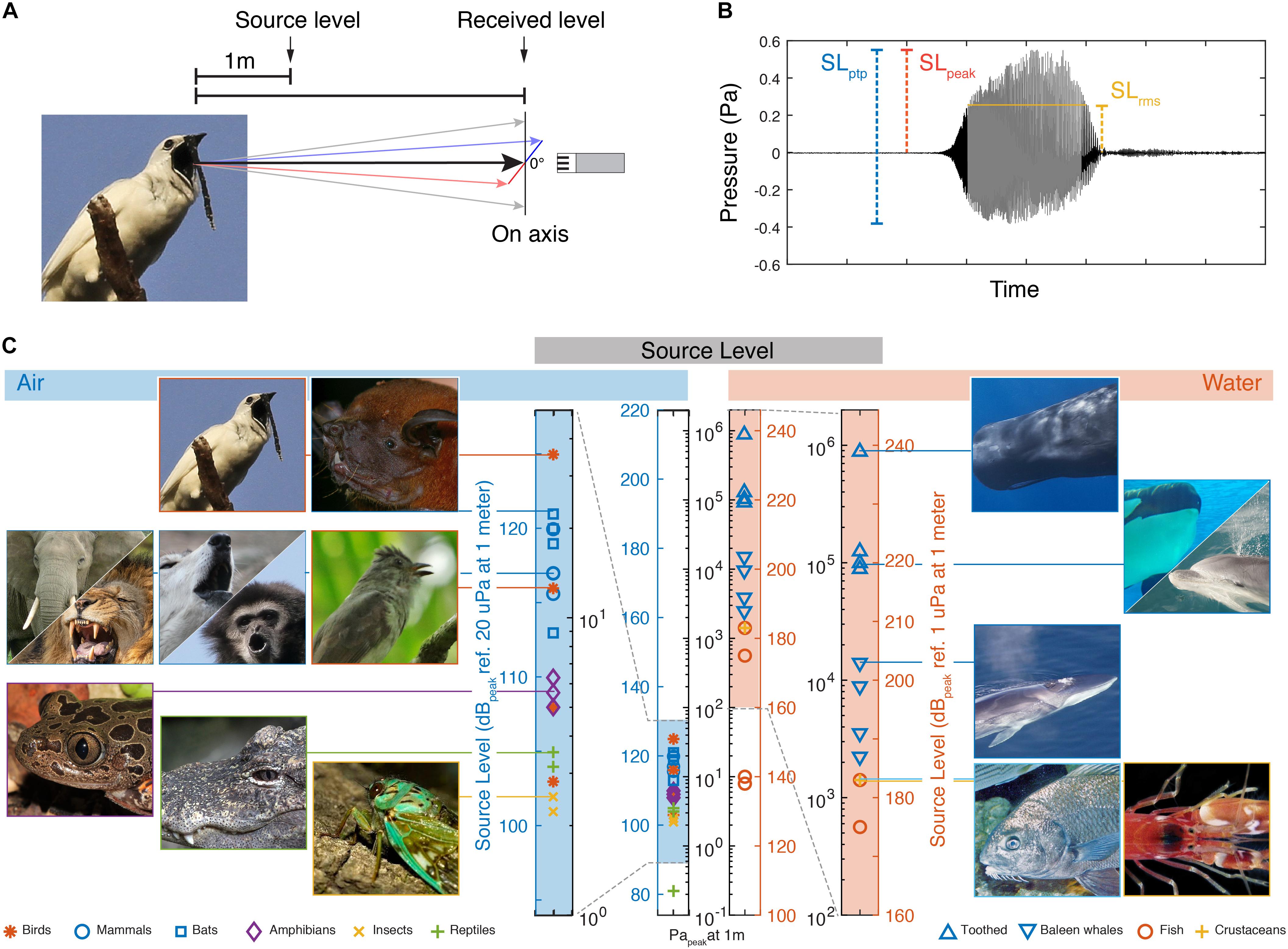
Figure 1. Source levels of the loudest animals in air and water. (A) Source level is defined as the on-axis radiated sound pressure at 1 m distance from the source. (B) Three commonly used measures of pressure amplitude; SLpeak is the highest absolute magnitude of the signal. SLptp is the difference between highest and lowest amplitude. SLrms is here shown as the rms amplitude over the duration set by using a 95% energy threshold criterion [see Madsen and Wahlberg (2007) for detail]. (C) SLs of the loudest reported animals in air and water (For data points and references see Table 1). The two vertical bars of pressure in the middle are on the same absolute pressure scale to allow direct comparison of the different dB scales in air and water.
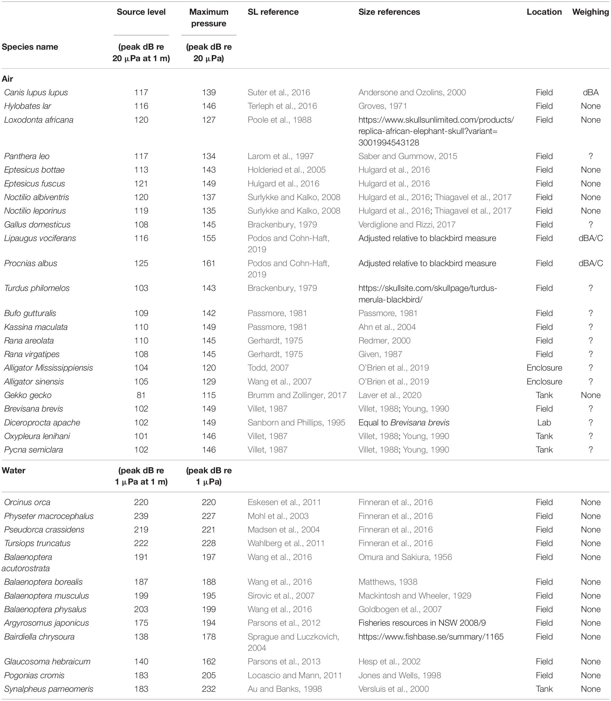
Table 1. Source level and maximum radiated pressures for animals in air and water.
First, the SI unit for pressure is the Pascal, but this physical property is often reported on the decibel (dB) scale, which first scales the data to a reference value and then applies a log transform. Because the reference value is typically 20 μPa in air and 1 μPa in water, the same absolute pressure in Pascal is represented by a numerical value 26 dB higher in water than in air when represented on the dB scale. To avoid confusion, we consistently report sound pressures both in Pascal and on the relevant dB scale (Also compare the two central pressure scales in Figure 1C).
Second, because it is not possible to measure the pressure at the location of the source, the SL is defined at some distance from the source. The reference distance varies between scientific fields but is one meter by convention in most biological and engineering applications. Many animals do not provide a convenient way to place a microphone or hydrophone at this reference position. In such cases, if the distance to the animal is known, the SL of the animal is estimated by accounting for the transmission-loss of the pressure magnitude over the distance traveled (Urick, 1983; Madsen and Wahlberg, 2007; Wahlberg and Larsen, 2017). Often simple spherical spreading loss models are used to estimate transmission loss, but these can be imprecise especially at longer distances to the source, when acoustical properties of the environment play an important role (Wahlberg and Larsen, 2017).
Third, because sound sources are directional at high frequencies relative to the size of the sound source, it is important to record the sound on-axis or to reconstruct the radiation directionality pattern and report the on-axis SL (Figure 1A). Sound pressure is highest along the acoustic axis and attenuates continuous with increasing off-axis angles. For highly directional sounds produced by bats and toothed whales the direction of the acoustic axis and position of the animal can be determined by using microphone or hydrophone arrays (Madsen and Wahlberg, 2007; Jakobsen and Surlykke, 2010).
Fourth, there are several ways to quantify the amplitude of a time-varying pressure wave. Amplitude measurements are traditionally either taken peak-to-peak (ptp), zero-to-peak (peak), or root-mean-square (rms) and it is important to note the differences when comparing studies using different amplitude measures (Figure 1B). For a sine wave, the peak-to-peak value is 6 dB higher than the peak and 9 dB higher than the rms value. For most real-world signals these relationships are different. Especially the rms amplitude will differ and the difference between peak-to-peak and rms can be greater than 9 dB depending on the time window used for computing the rms. Sound level meters are also used for bioacoustics measurements and common measures are given as either Lpeak or Leq. Lpeak equals the peak amplitude measurement with no time averaging applied and is used widely in bioacoustics and human audiology research. Leq is the equivalent continuous level and the same as the rms measure.
Fifth, the frequency response and sensitivity of the recording chain needs to be specified. For example, most sound level meters have different filters that can be selected, e.g., A, C, and Z weighing, where A and C relate to human loudness perception at different intensity levels, and Z has a constant reference pressure of 20 μPa across frequencies (i.e., unweighted) (International Standard IEC61672-1, 2002). Thus, A and C weighing can be used to make conclusions about human perception. Because hearing sensitivity varies significantly across species this type of weighing should be avoided in bioacoustics research and will especially affect low- and high-frequency sounds. Lastly, sound level meters come in two classes, 1 and 2 that have difference tolerance limits for precision. Both perform almost equal between 20 Hz and 10 kHz, but class 2 has lower precision tolerance outside this frequency range. Therefore class 1 sound level meters are recommended for measurements at frequencies below 20 Hz and frequencies above 10 kHz.
Which Animals Produce the Highest Source Levels?
To identify the loudest species, i.e., the species that produce the highest SLs, within and between all clades of vocal animals in air and water, we compiled SLs of animal vocalization per taxon (see section “Materials and Methods,” Figure 1C and Table 1). To prevent overrepresentation of species with lower SLs, we included only the four loudest species within each taxon. We included bats and toothed whale as separate groups because echolocation likely imposes a different evolutionary demand on the sound production system than does communication. The variable measuring conditions of acoustic fields in laboratory and field, makes comparing dB values with precision below 1 dB not very meaningful. In combination with the different methodologies used to measure peaks or average maxima, we should consider the maximal values reported here indicative within 2–3 dB of what the animals produce. Our efforts in trying to compile these data emphasized to us how infrequent SLs are reported in bioacoustics papers. Given the importance of SL for the biology of species, we thus would like to urge people to measure and report SL in their work.
In air, the loudest reported animals are birds and mammals. The White Bellbird (Procnias albus) is the loudest at 125 dBpeak re. 20 μPa at 1 m (i.e., 36 Papeak at 1 m) (Podos and Cohn-Haft, 2019). Elephants and bats are runners up at 120 dBpeak re. 20 μPa at 1 m (i.e., 20 Papeak at 1 m) (Poole et al., 1988; Surlykke and Kalko, 2008; Hulgard et al., 2016). The loudest reported amphibian species call at 110 dBpeak re. 20 μPa at 1 m (i.e., 6.3 Papeak at 1 m) (Gerhardt, 1975; Passmore, 1981). The loudest reported reptile species are the alligators at around 105 dBpeak re. 20 μPa at 1 m (i.e., 3.6 Papeak at 1 m) (Todd, 2007; Wang et al., 2007). The loudest reported insects are several species of cicadas at 102 dBpeak re. 20 μPa at 1 m (i.e., 2.5 Parms at 1 m) (Villet, 1987; Sanborn and Phillips, 1995). These SLs represent the highest values at species level. For the bat, bird, insect and toothed whale species included here, the SL values reported represent their reported loudest vocalizations. However, for the other species we do not know if the reported SLs encompass the maximal capabilities in the species-specific vocal repertoire, and we cannot exclude they can emit higher SLs.
Also within species, SL variability can be expected. Humans deserve special attention because it is the only species where we have some information on the loudest individuals within a species. The human shouted voice is about 105 dBrms re. 20 μPa at 1 m (Lagier et al., 2017). However, The Guinness Book of World Records lists the loudest voice from a schoolteacher saying “Silence” at 122 dB re. 20 μPa at 1 m and the loudest non-speech scream to be 129 dB re. 20 μPa at 1 m, which would rank humans up with the loudest mammal and birds. However, we have not been able to confirm the recording methodology of these records with Guinness, including what amplitude measure was used, and therefore do not include them here. Taken together, in air, the loudest animals all emit surprisingly similar maximum SLs around 120 dBpeak re. 20 μPa at 1 m, which equals 20 Papeak at 1 m.
In water, maximum SLs are much higher than in air. Toothed whales are by far the loudest group of animals in water; the sperm whale (Physeter macrocephalus), emits echolocation clicks with SLs up to 239 dBpeak re. 1 μPa at 1 m (i.e., 900,000 Papeak at 1 m) (Mohl et al., 2003). In comparison, the loudest baleen whale is the fin whale (Balaenoptera physalus) at 203 dBpeak re. 1 μPa at 1 m (i.e., 14,000 Papeak at 1 m) (Wang et al., 2016). The loudest teleost fish, the black drum (Pogonias cromis) (Locascio and Mann, 2011), is almost three orders of magnitude of pressure below the sperm whale at 183 dBpeak re. 1 μPa at 1 m (i.e., 1,400 Papeak at 1 m), as is the pistol shrimp (Synalpheus parneomeris) at 183 dBpeak re. 1 μPa at 1 m (Au and Banks, 1998). Please note that the dB values in water are 26 dB higher than in air due to the difference reference pressure of 1 μPa alone (see central, black labeled pressure scale in Figure 1C). In water, we thus do not observe that different animal clades converge upon a maximum SL.
Loudest Animals Are Independent of Size and Frequency in Air, but Not in Water
How much would a sound source need to move to achieve a SL of 125 dBpeak re. 20 μPa in air or 240 dBpeak re. 1 μPa in water? To approximate this, we considered the output of two simple sound sources: (1) a pulsating sphere and (2) a piston of equal diameter (see section “Materials and Methods,” Figure 2). These models show that the velocity needed to achieve a certain fixed SL decreases with the radiated frequency and physical size in air and water (Figures 2A,B). We also considered the product of the wavenumber (k = 2πf) and size (a), the ka product. This dimensionless parameter represents the acoustic size of an emitter i.e., the size relative to the wavelength it is emitting since ka = 2πa/λ. At a fixed SL, the velocity also decreases with ka for both air and water (Figure 2C). While the piston model shows a power relationship (linear on the double logarithmic axes), for the pulsating sphere the velocity required becomes constant at higher frequency, size and ka. This is because the source becomes large compared to the wavelength and tends to locally radiate a plane wave, for which the ratio of sound pressure to particle velocity is the characteristic impedance of the propagation medium, ρc [see also Equation (1) in section “Materials and Methods”]. By fixing other parameters, such as rms volume velocity of the source (see section “Materials and Methods”), the SL increases with frequency, size and ka product (Figures 2D–F). Again, for the pulsating sphere, the SL does not increase with frequency, size and ka for a fixed velocity over a certain frequency for the reason mentioned above.
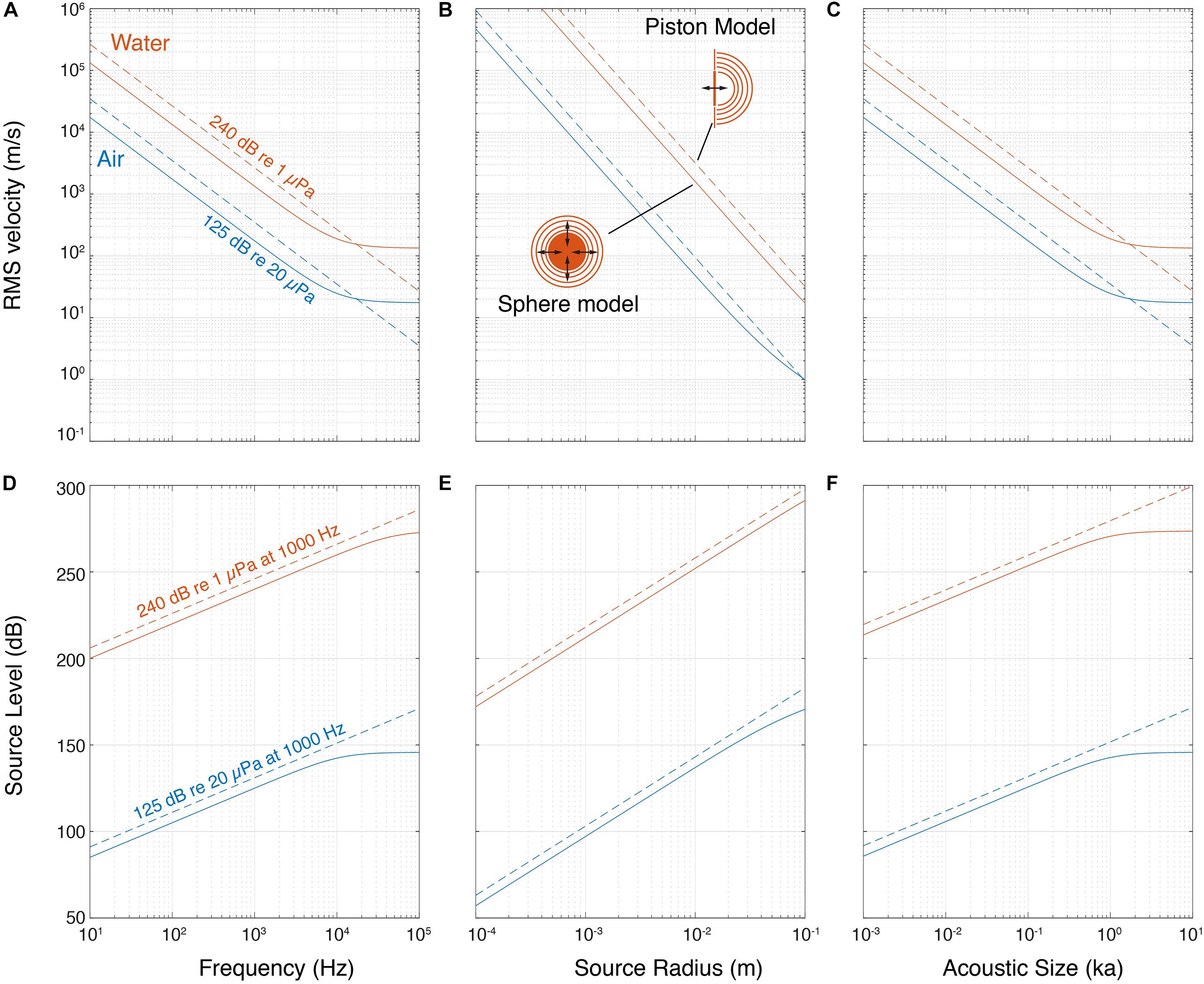
Figure 2. Pulsating sphere and piston models predict that source level depends on frequency and size. (A) Isolines of a 240 dB re. 1 μPa and 125 dB re. 20 μPa source show that producing sound requires less movement with higher frequency, (B) size and (C) ka product. (D) SL increases with frequency, (E) size and (F) ka product for both sphere and piston models. The lines shown here are at a volume velocity that makes the source of 10 mm diameter produce 240 dB re. 1 μPa and 125 dB re. 20 μPa at 1,000 Hz, in water and air, respectively (see section “Materials and Methods”).
These simple models illustrate three acoustic considerations important for generating sound. First, to produce higher frequencies at the same SL, the source needs to move less. Second, reversely, with the same source velocity, a higher SL can be achieved at higher frequencies or larger size. Third, due to the impedance difference between air and water, the same source motion results in water in a three orders of magnitude higher sound pressure than in air. It is thus much easier to generate a high pressure in water.
The ka product determines how much of the power used to produce the sound is converted into acoustic power that radiates from the source, i.e., the efficiency of the source. For a pulsating sphere the maximum efficiency is at ka ≥ 2. Below ka = 2 efficiency drops by 100 for every order of magnitude of ka (Michelsen, 1992; Larsen and Wahlberg, 2017). While there is no increase in source efficiency at ka > 2, most sound sources will exhibit a substantial increase in SL because the sound source becomes increasingly directional with increasing ka, i.e., pressure is highest along the acoustic axis and progressively decreases at greater off-axis angles. Thus, a directional source radiating the same acoustic power as an omni-directional source will emit a higher SL on the acoustic axis. However, a pulsating sphere does not become directional at high ka.
Because these simple acoustical models predict a clear dependency on frequency, size and ka product, we compiled SL of the loudest animals as a function of their peak frequency body mass, acoustic radius and ka product (Figure 3 and Supplementary Table 1, see section “Materials and Methods”). We consider that applying descriptive statistics is not meaningful given the sparse nature of the data, but a few patterns do emerge. Although within a clade body size may be a good predictor of SL (Villet, 1987), for the loudest aerial species we observe no increase of highest SLs with radiated sound peak frequency over four orders of magnitude (Figure 3A), no increase with body mass across nearly five orders of magnitude (Figure 3B) and no increase with increasing ka over two orders of magnitude (Figure 3D). All loud insects, frogs, reptiles, birds and terrestrial mammals have ka between 0.1 and 1, which makes them omnidirectional sound emitters. The bats have ka > 2, which makes them efficient and more directional sound emitters. Thus, in contrast to simple linear acoustic models that show increase of SL with increasing frequency, radius and ka product, the maximal SL of around 120 dB re. 20 μPa at 1 m in air seems independent of weight, radius, frequency and ka product (Figure 3 and Supplementary Table 1).
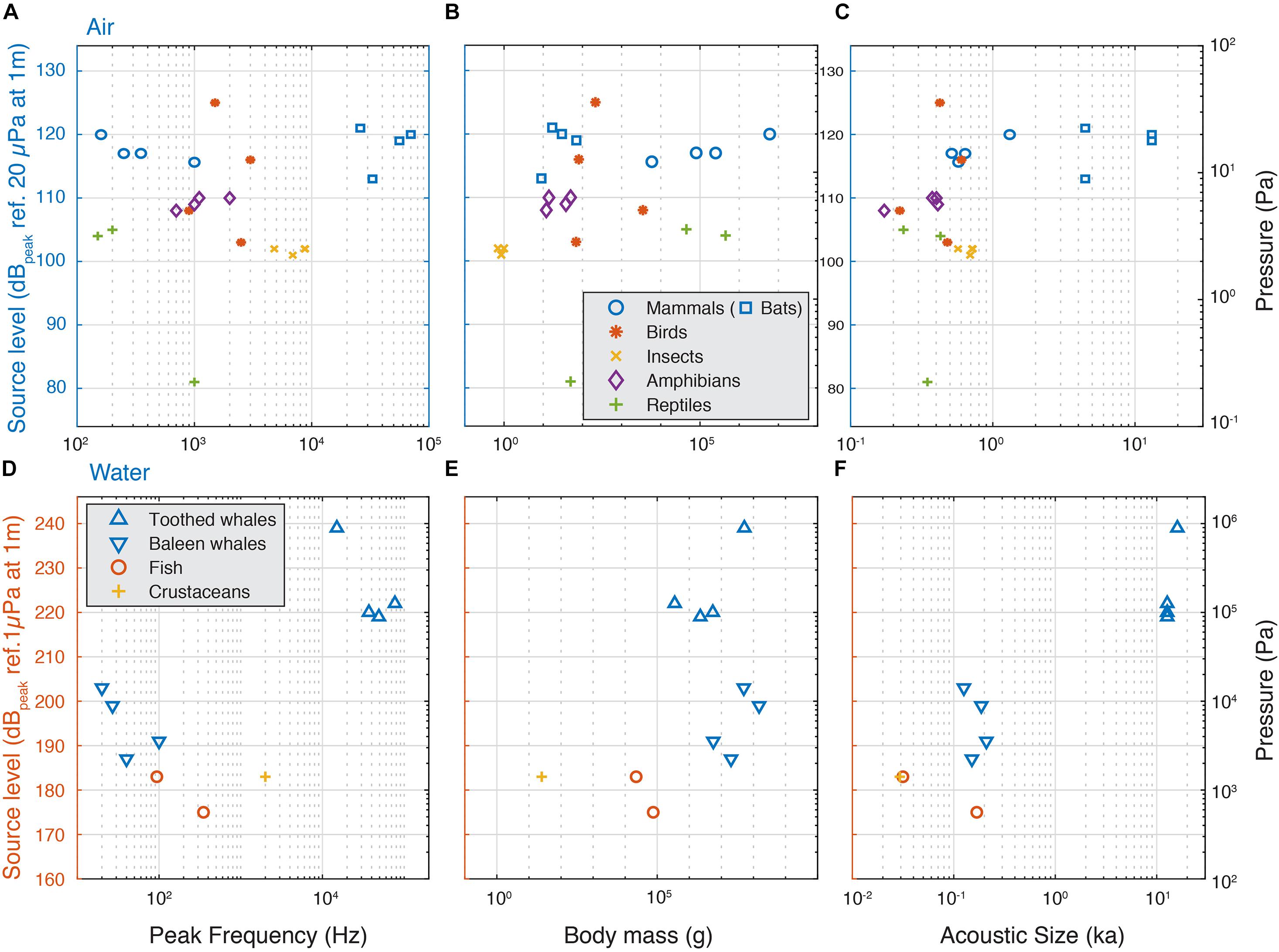
Figure 3. Source levels of the loudest animals do not increase with frequency, weight and acoustic size in air, but do underwater. (A) The highest SLs do not increase with frequency, (B) body mass or (C) ka for animals vocalizing in air and is maximally 125 dB re. 20 μPa at 1 m. (D) In aquatic animals, we observe a trend that the highest SLs increase with frequency, (D) in aquatic animals, we observe a trend that the highest SLs increase with frequency, (E), body mass and (F) ka, but the sparsity of the data prevents statistical interpretability.
For aquatic animals, the sparse observations fit the simple acoustic models that highest SL increases with frequency (Figure 3C), body size (Figure 3D) and ka product (Figure 3E). However, due to the sparseness of the data, we should be cautious interpreting this data. For loud crustaceans, fish and baleen whales, the ka product is between 0.01 and 0.2, which makes them omnidirectional, but not such efficient sound emitters. For tooth whales the ka product is larger than 10, which makes them efficient and highly directional sound emitters. As a consequence, while toothed whale SLs are substantially higher than the baleen whales, the high directionality means that the difference in radiated acoustic power, i.e., the combined sound radiation in all directions, is much smaller. This is because when emitting sound directionally, sound pressure is concentrated in the frontal direction and much lower pressures are radiated off-axis whereas for omni-directional sources, sound pressure radiation is roughly equal in all directions.
Physical Upper Limits to Sound Pressure Generation and Radiation
The SL of bat echolocation calls has been suggested to be close to the physical limit of maximal pressure generation in air (Madsen and Surlykke, 2014). Are animals indeed so loud they are hitting certain physical limits to sound production?
In air, pressure fluctuates around atmospheric pressure of about 100 kPa and the negative crest is limited at 0 Pa. Sound waves that are symmetric around atmospheric pressure can therefore reach an amplitude of maximally 200 kPa peak-to-peak (194 dBpeak re. 20 μPa). However, there is no theoretical physical upper limit to pressure, and extreme explosions can indeed surpass the 100 kPa positive crest. The supposed loudest explosion in recent human history was the 1883 Krakatoa volcano eruption with an estimated SL of about 270 dBpeak re. 20 μPa at 1 m (Winchester, 2003). Besides many issues with approximating this particular SL, it is clear that in air, making sounds by exploding is not a viable option for animals, and vocalizations do not reach such enormous pressures.
In water, the minimal sound pressure is limited by the formation of vapor-filled cavities, i.e., cavitation, at 0 Pa. Because the ambient water pressure depends on depth in the water column, the difference between ambient pressure and cavitation also depends on diving depth. Thus, a sound wave at the water surface and symmetrical around atmospheric pressure can therefore also reach an amplitude of maximally 200 kPa peak-to-peak (220 dBpeak re. 1 μPa). Again, there is no theoretical upper limit to pressure, but because the cavitation boundary poses a design constraint in human-made sonar systems (Woollett, 1962) it is reasonable to assume that this also is the case for biological systems. A sperm whale click of 239 dBpeak re. 1 μPa would thus actually surpass the minimal crest limit when produced at shallower depths than 80 m.
The above physical limitations apply to acoustic pressure magnitudes irrespective of where they occur in the sound field of a source. However, what are the maximal sound pressures animals produce in the entire sound field that they radiate? Whereas SL is defined at the reference distance of 1 m, the highest pressures mostly occur much closer to most animals. To estimate the maximal acoustic pressures the loudest animals generate, we approximate them as two types of sound sources; a pulsating sphere and a piston in an infinite baffle (Figures 4A,B). In the far field sound pressure decreases with 6 dB per doubling of distance due to the spreading of the acoustic power over a larger area (Jacobsen and Juhl, 2013). A pulsating sphere only has a far field and the highest pressure produced is obtained at the surface of the sphere (Figure 4A, see section “Materials and Methods”). However, pistons and more complex sound sources also have a near-field where the pressure strongly depends on local conditions. For a piston in an infinite baffle the transition from near to far field boundary can be conservatively approximated by: Dpiston = k×a2, where k is the wavenumber (k = 2π/λ) and a the radius of the emitter (Figure 4B; Foote, 2014). In the interference near field of a piston, pressure can be up to 12 dB higher than are the near/far field border we use for our approximation and strong dips occur that are highly sensitive to local conditions and ka-values (Figure 4B). Given the near field conditions are very specific for each animal, we consider it safer to use the more conservative maximum pressure at the boundary between the geometric nearfield and the far field.
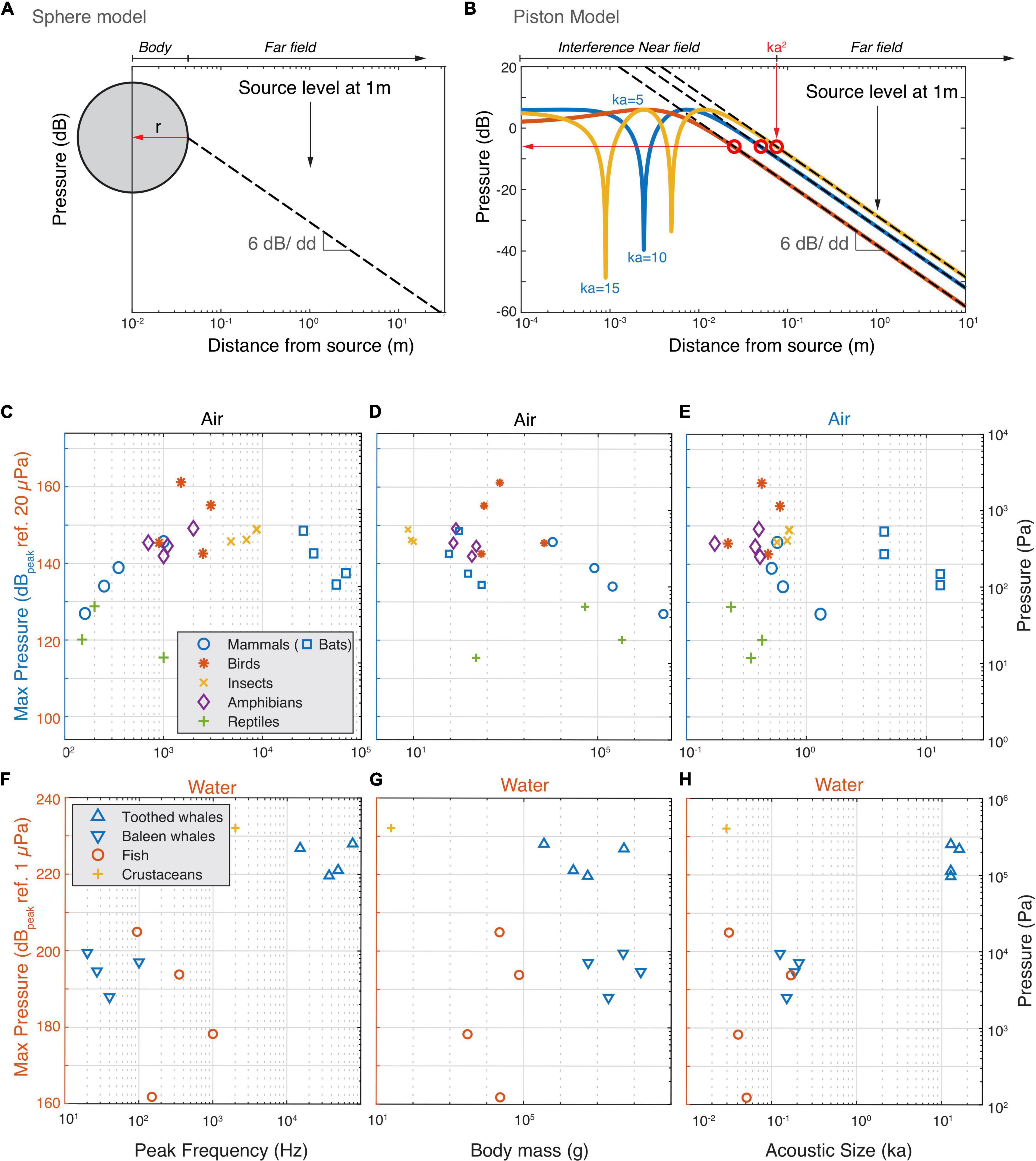
Figure 4. The estimated highest occurring sound pressures in air and water. (A) For animals that are omni-directional sound radiators we used the monopole model to estimate the highest occurring pressure (red horizontal arrow). Because a monopole does not have a near field, we assumed the radius of the monopole to be the body wall (see section “Materials and Methods”). In far field conditions, the sound pressure decreases with 6 dB per doubling of distance. (B) For highly directional sound radiators (bats and cetaceans), we used the piston model to estimate the highest occurring pressure. We use the conservative estimate that the highest occurring pressure (red horizontal arrow) occurs at the border of the interference near field and far field (see section “Materials and Methods”). (C–E) Estimated highest produced sound pressures increase with frequency but plateau at about 150 dB ref. 20 μPa by animals vocalizing in air. (F–H) Estimated highest produced sound pressures seem to increase with frequency and size for animals vocalizing in water.
Using these two models, we estimated the maximum pressures the loudest animals generate (see section “Materials and Methods”). In air, below 2 kHz the estimated maximum sound pressure increases with frequency (Figure 4C). However, at 2 kHz, the pressure seems to reach a plateau at 150 dBpeak re. 20 μPa with the exception of the Bellbird that reaches 160 dBpeak re. 20 μPa. This maximum pressure plateau is also maintained for animals under 10 kg but decreases with body mass over 10 kg (Figure 4D) and radius over 5 cm (Supplementary Table 1). When estimating the maximum pressure produced, the frogs and cicada’s move up and interestingly, all loudest mammals, birds, cicada’s and frogs converge upon 140–150 dBpeak re. 20 μPa. In water there is a trend that maximum pressure increases with frequency with no indication of a plateau as seen in air (Figure 4F). However, body mass, and ka product do not show clear relationships with the maximal pressure (Figures 4E,F). Both the pistol shrimp and the toothed whales produce estimated maximal pressures as high as 230 dB re. 1 μPa and reach cavitation limit pressures at depths less than 30 m.
Taken together, we observe that animals vocalizing in water roughly follow the source relations predicted by sphere or piston models. The loudest animals in water come close or reach a physical limit (cavitation) when producing loud sounds at shallow depths. The loudest animals vocalizing in air are efficient sound producers, but do not get close to the maximal amplitude for a symmetrical wave. Our data thus suggests that they are limited to amplitudes of 140–150 dBpeak re. 20 μPa.
Physical Upper Limits to Sound Propagation
The next physical limitation of sound production is the phenomenon that at high acoustic pressures sound propagation becomes non-linear and efficacy decreases. The non-linearities occur since the speed of sound is temperature dependent and pressure fluctuations are accompanied by temperature fluctuations. As a result, the positive pressure crest travels faster than the negative pressure crest. This effect accumulates over distance and eventually (depending on loss mechanisms) shockwaves may form, even from a waveform that is initially a sinusoid (Pierce, 1981). This distance from the source at which the shock wave is formed is called the shock formation distance. The relevant propagation (e.g., communication or prey detection) distance is thus a key factor to include when estimating shock formation distance. The creation of shockwaves is frequency and level dependent and the radiated waveshape at the source also plays a major role. The sound producing process itself might lead to a waveform that is close to that of a shockwave, thereby reducing the shock formation distance. Because of these propagation non-linearities, very loud sounds attenuate much more rapidly with distance than dictated by simple spherical spreading loss and atmospheric attenuation. The introduction of propagation non-linearity can (depending on level, frequency, and range) even give rise to a saturation effect for sound propagation in air and water, because increased SL beyond this level is not associated with an equivalent increase in signal range (Pierce, 1981).
However, the effects of spherical spreading and absorption counteract the formation and propagation of shockwaves. Since absorption in both air and water increase with frequency, the higher harmonics caused by the transition into a shockwave are attenuated more than the fundamental frequency leading to a sinusoidal waveform at large distances (the so-called old-age region) (Pierce, 1981). The strength of this counteracting effect depends on amplitude, frequencies and propagation distances. This effect along with the saturation effect is in particular relevant for animals communicating over long distances.
Shock wave formation can thus be considered a realistic but “soft” limit to sound production in air and water, because it is frequency, level, waveshape and distance dependent. Due to the complicated non-linear acoustics involved, analytical models of the attenuation of shock waves are limited to approximate cases such as plane wave propagation of an initially sinusoidal waveform. As a rule of thumb and at moderate distances, sound pressure can reach 150 dB ref. 20 μPa in air and 240–250 dB ref. 1 μPa in water before physical non-linearity and additional losses significantly reduce amplitude (Larsen and Wahlberg, 2017). Thus at least in air, the loudest birds, mammals, frogs and insects create sound pressure levels that approach the level at which non-linear propagation losses become significant and further increase would be inefficient as a mean to increase communicative distance. Thus, radiation non-linearities may provide a realistic physical limitation to making louder sounds. The resulting skewed sound waveforms are at least consistent with the bellbird calls and mammalian screams.
Definitively answering the question if propagation non-linearities are physically limiting sound production requires non-linear modeling and precise measurements. The acoustic nearfield and spherical spreading have to be taken into account and can only be solved numerically. Measurements of shock waves and thereby high-order harmonics from animals producing high-frequency vocalizations should be definitive, but also impose high demands to the equipment in terms of sampling frequency and transducer response. The conditions are so different for each species that the question must be solved on a case-by-case basis, which is beyond the scope of this paper.
Physiological Limitations to the Production of Loud Sounds
All extant vocalizing species have undergone millions of years of evolution and sound production is only one of a multitude of trade-offs individuals face in their survival. Many factors could thus play an important role in explaining why most species do not produce loud vocalizations. First of all, making high acoustic pressures is also conspicuous and thus not necessarily an advantage. Another major factor is the energetics and efficiency of vocal production in relation to the ecology and behavior of a species. In frogs, birds, and bats it has been shown that high SLs come with a substantial increase in energy expenditure (Currie et al., 2020). Obviously, the duty cycle of calling plays a major factor in this; some frog species call at high duty cycle for several hours, but other species may only produce a few vocalizations per day. However, if power plays a major role, we would hypothesize that large animals would be louder as they could afford more energy, but our data does not support this. Additionally, loud sounds can become too loud and may temporarily deafen the receiver (Finneran, 2015). These are just a few reasons why an animal may not invest in making high sound pressures. However, can we identify more principal constraints in the physiology that pose a limitation to producing high sound pressures?
To answer this question, we need to look at the different mechanisms animals use to generate sounds. Sound production mechanisms differ widely and pose phylogenetic and evolutionary constraints. In some case they are not well-understood or even unknown. Most air-breathing tetrapods produce vocalizations by converting respiratory flow to modulated flow by self-sustained oscillation of laryngeal vocal folds or syringeal analogous structures. The resulting air pressure disturbances constitute the acoustic excitation of the system (Titze, 2000). This framework is called the myo-elastic aerodynamic theory of sound production or MEAD. The theory of sound production using MEAD is best studied in humans, but also found applicable to non-human mammals (Herbst et al., 2012) and birds (Elemans et al., 2015; Jiang et al., 2020). Amphibians and the few vocal reptiles probably also use MEAD (Rand and Dudley, 1993; Reber et al., 2015).
We identified at least four MEAD features that potentially pose limits to producing high SLs. A first limit is the efficiency by which aerodynamic energy is converted into acoustic energy. This efficiency is referred to as the glottal efficiency in laryngeal sound producers including humans (van den Berg, 1956; Bouhuys et al., 1968; Schutte, 1980) or vocal/mechanical efficiency (ME) (Titze et al., 2010; Zhang et al., 2019) and is defined as the ratio of radiated acoustic power over driven aerodynamic power of the subglottal/subsyringeal air. Acoustic power is typically determined by combining the measured sound pressure, impedance and an approximation of the area over which the energy is radiated. Aerodynamic power is calculated as the product of measured mean tracheal/bronchial airflow and pressure. When measured in vivo, ME captures both (i) the transformation of aerodynamical power into acoustic flow within the vocal tract, (ii) transmission efficiency through the airways, and (iii) the transformation of sound from the surface (mouth/beak/air sacs) to the environment (Titze and Palaparthi, 2018). ME varies greatly with bronchial pressure (Herbst, 2014), frequency (Zhang et al., 2019), vocal fold position, geometry and pathologies and also in between species (e.g., Brackenbury, 1979; Titze et al., 2010; Herbst, 2014; Maxwell et al., 2021) and values are reported between 10–4 to 2% (e.g., a factor of −60 to −20 dB).
Many animals have evolved anatomical or behavioral adaptations that aid in radiating the sound energy from their vocal organs to the radiated sound field. Indeed, the ME of excised vocal organs is typically lower because there is no upper vocal tract (Titze, 2006). Anatomical adaptations to increase sound radiation efficiency, such as air sacs in frogs (Rand and Dudley, 1993), birds (Riede et al., 2004), and mammals (Riede et al., 2008), or enlarged larynges in howler monkeys (Dunn et al., 2015) and hammerhead bats (Schneider et al., 1967). Additionally, behavioral adaptations can be found such as posture modifications to increase mouth/beak opening when emitting high SLs, as seen in the bell bird and, howler monkeys. Models suggest that for mammals and birds, adjustments of head size, mouth opening, and beam direction can make the power transformation efficiency from vocal tract to radiated sound as high as 100% in the 1–50 kHz range (Titze and Palaparthi, 2018). Some animals even change their environment by constructing horns or baffles that aid in radiating the sound (Mhatre et al., 2017).
A second limitation is the amount of aerodynamic energy an animal can produce. in vivo and excised larynx and syrinx work has shown that SL increases with mean bronchial pressure (Schutte, 1980; Zhang et al., 2019). The increasing pressure leads to higher VF displacement, sharper flow starts and stops and therefore a higher SL. The maximal expiratory pressure is limited by the maximal effort of respiratory muscles and in humans ranges from 5 to 7 kPa during crying in infants and up to 10–15 kPa in adults during shouting (Wilson et al., 1984; Dimitriou et al., 2000; Lagier et al., 2017). Without vocalizing, higher expiratory pressures over 20 kPa can be achieved by both normal and brass instrument playing adults (Fiz et al., 1993).
However, before the maximal respiratory pressure or flow is achieved, a third limit is typically reached. As bronchial pressure and flow increases, at specific values the dynamics of VF vibration behavior bifurcates from regular to chaotic regimes. This point is called the phonation instability pressure or flow (Jiang and Titze, 1993; Hoffman et al., 2012). As pressures exceed the phonation instability pressure (PIP) the SL does not increase further in the few species studied (Jiang and Titze, 1993; Zhang et al., 2007; Hoffman et al., 2012), probably because the vocal efficiency decreases. Although using pressure above the PIP is unfavorable from an energetics point of view, irregular or chaotic vocal fold regimes are common in mammalian vocalizations (Wilden et al., 1998; Fitch et al., 2002) and their signaling function in communication thus likely outweighs the loss of energy efficiency.
Fourth, with increasing amplitude the collision force of vocal folds, or impact stress, increases. Although short peak impacts may not be a limiting factor per se, accumulative vocal fold damage due to a large amount of high impacts, aka the vibration doses, may be limiting. Through intense voice use, damage can accumulate over time and tissue stress is suggested as the tradeoff for peak performance (Titze and Hunter, 2015). Impact stress is also the main traumatizing mechanism in human voice production, and the main cause of vocal fold nodules (Horacek et al., 2009). In humans, many impact related VF pathologies are known, but to our knowledge there is no reports on VF pathologies in animals.
Taken together, for animals using MEAD to produce vocalizations, at least the above four physiological constraints could pose limits to SL. However, we suggest that these constraints are not hard limits, but should be more seen as trade-offs in energy expenditure or vocal fold damage. Furthermore, our current dataset does not allow investigation of allometric scaling with anatomical and physiological parameters (e.g., Charlton and Reby, 2016), because we did not systematically sample across a range of SLs and taxa that use MEAD. Instead we specially mined the literature for the highest SLs. It would be interesting to see if within phylogenetically related taxa of animals using MEAD allometric relationships can be found, as between SL and size within the cicada’s (Villet, 1987).
The loudest insects, the cicadas, use a fundamentally different mechanism to produce sound. Cicada’s buckle ribs on their tympanum that results in clicks, which provides a resonant source that drives the abdominal resonator, from which sound is radiated via the tympana (Young and Bennet-Clark, 1995). The limit to produce clicks is unknown, but most likely related to mechanical failure of the tympanic ribs.
Animals producing loud sounds in water do so by at least three mechanisms. The unique mechanism by which pistol shrimp produce sound using their large snapper claw is well-understood. Muscle co-contraction builds up tension that is released by contraction of another muscle. The rapid closure of the claw pushes a plunger into a socket, and creates an outward water jet at such velocity that a cavitation bubble forms. It is the implosion of this cavitation bubble that creates the loud snapping sound (Versluis et al., 2000).
Bony fishes have evolved perhaps the largest diversity of sound generating organs among vertebrates (Fine and Parmentier, 2015; Ladich and Winkler, 2017). For the few species studied, the most common mechanisms are muscle driven vibration of a gas-filled bladder, and stridulation mechanisms of pectoral girdle or fin (Ladich and Winkler, 2017). The loudest teleost fish reported here most likely produce sound by swim bladder vibration (Locascio and Mann, 2011). Because all vertebrate muscles trade-off muscle power and speed, the fastest muscles can move at rates of 270 Hz (Mead et al., 2017). These extreme contraction rates still produce low frequencies for sound. Given the size of the fish, these result in ka < 1, which makes them poor pressure radiators. However, many fish are mostly sensitive to particle motion, not pressure, and thus pressure may not be the most relevant cue for communication (Radford et al., 2012).
In cetaceans sound production has received much attention, however, we have no convincing direct evidence of how the sounds are produced. Cetaceans have shared ancestry with the artiodactyla and sound production is thought to be driven by air flow. In mysticetes, the hypothesis that sound is produced by laryngeal tissue vibration is based on anatomy (Damien et al., 2019) and we still lack direct experimental observation to test outstanding hypotheses. Their relative low ka values make them suboptimal sound radiators, but the low-frequency emission may be favorable because of low absorption and thus allow long-range communication. The odontocetes produce the highest sound pressures of all animals (Mohl et al., 2003). Several lines of evidence suggest that sound production occurs at the phonic lips in the upper nasal passages, either by a muscle-driven catch-release mechanism or an air-flow driven MEAD system. The sound radiates from the melon is highly directional. In the sperm whale, the produced sound is collimated inside the enormous nasal complex, resulting in the most directional sound source known where most energy is concentrated in a beam of only a few degree (Mohl et al., 2003). However, given the fact that odontocetes are producing the highest sound pressures of any animal on the planet especially warrants further investigation to understand how they manage to produce 1 MPa sounds.
Conclusion
Across the animal kingdom we find that the loudest animals span several orders of magnitude of size and frequency and can be found in all phylogenetic groups and habitats. To investigate what potential mechanism could limit the generation of loud sounds, we compiled SL data for animals vocalizing in air and water. In air we see that SLs are limited to 125 dBpeak re. 20 μPa at 1 m after correcting for scaling conventions. The maximum actual pressure generated are 140—150 dBpeak re. 20 μPa, typically much closer to the source than one meter. Several physiological processes could be limiting but given the many tradeoffs the different animals face during evolutionary history it is hard to point to a single constraint that explains the maximally observed values. Two physical constraints are of a magnitude to pose serious limitations. First the acoustical size (ka) constraints the efficiency of sound radiation. The loudest animals in air all seem to be good radiators, maybe except for the elephant, with ka close to or above 1. Second, non-linear propagation makes it inefficient, but not impossible, to make louder sounds. Thus, in air, physical limitations and particularly non-linear propagation could play a major role in how loud animals can maximally get.
In water, pistol shrimp and odontocetes produce extreme acoustic pressure close to the zero pressure (cavitation) limit. The loudest fish reach a physiological limit that muscle-powered swim bladder motion is limited to generating frequencies of 300 Hz. The mechanisms of sound production in both baleen and tooth whales are not well understood. How these animals achieve these incredible SLs is not well known.
Being loud is one of many strategies of the surprising tapestry of animal vocalizations. The loudest animals produce sound pressures where several physical processes become highly non-linear. To solve which process poses a limitation to producing higher SLs requires the development and detailed testing of numerical models on a case-by-case basis. Although for the majority of animals, being loud has not been an evolution strategy, we see that both in air and in water, species have evolved that are pushing against the physical limits of sound production.
Materials and Methods
Source Level Comparison and Compilation
We determined SLs by making the following two conversions to the literature data if relevant: First, we use sound pressure level (peak) as the proxy for sound amplitude (Figure 1A). For the particular purpose of this study, peak is a better measure than RMS because it represents the maximum pressure the animals are producing while RMS averages the pressure over the duration of the sound. We did this conversion using the relationship between peak, peak-to-peak and RMS for a simple sinusoid, i.e., by adding 3 dB to RMS values or subtracting 6 dB from peak-to-peak values. For RMS values this underestimates the peak value for non-sinusoid signals, which makes our SLpeak values conservative estimates. Second, we calculate SL to the standard reference distance of 1 m using spherical spreading attenuation. While atmospheric attenuation becomes substantial in air at frequencies >20 kHz, it is negligible over the short distances we encounter here and very likely less than the overall uncertainty involved in the reported measures. All our values are based on the highest reported values in each study.
Pulsating Sphere and Piston Model
To relate sound pressure measurements at one position to another we must adopt a model of the sound source and the propagation medium. For the medium we assume lossless free space and discuss air/water-attenuation at ranges where these effects are relevant. For the sound source we employ two models: the pulsating sphere and the piston in a baffle, which despite being simple approximations are quite often used in bioacoustics.
For a pulsating sphere the relation between pressure amplitude and surface velocity is (Jacobsen and Juhl, 2013):
where ρ is the density of medium, c is the speed of sound in medium, wavenumber k = 2π f/c,
a is the radius of the sphere, U is the velocity of the sphere surface and r is the distance to center of sphere. If the velocity is given as an RMS value, the resulting sound pressure is an RMS as well and so forth for peak or peak-to-peak values. The quantity (4πa2 U) is the volume velocity of the sphere, which is often used to characterize source strength in acoustics.
For a piston in a baffle, we limit the discussion to the on-axis pressure, the amplitude of which can be calculated by, (Jacobsen and Juhl, 2013)
where x is the distance to the center of the piston. For high frequencies and close distances strong interference can occur (Figure 4B), whereas an approximate expression can be found for long distances (compared to both radius and wavelength):
Note that the volume velocity of the piston, (πa2 U), is one-fourth of that of the sphere.
For a given radius and volume velocity, the frequency response of the sphere is increasing by 6 dB/octave at low frequencies before reaching a limit at ka = 1 (3 dB corner frequency). For the piston in a baffle, there is no such limit in the far-field, but evidently the near-field extends further with increasing frequency.
Estimation of Maximal Acoustic Pressure
For sources that can be considered equivalent to oscillating pistons, we used the theoretical boundary between the interference near field and far-field as the distance to the source where the highest sound pressure occurs. According to Foote (2014), this can be approximated conservatively as:
Where a is the radius of the piston and λ is the wavelength of the sound. We use this approximation for the toothed whales and bats who’s highly directional sound emission patterns have been shown earlier to fit well with piston model predictions (see e.g., Mohl et al., 2003; Jakobsen and Surlykke, 2010). For bats we used the piston-fit to the measured directionality of E. fuscus as reported in Hulgard et al. (2016). We assumed that E. bottae emits similar directionality to E. fuscus and computed a using emitted frequency as reported by Holderied et al. (2005). For The two Noctillio, we assume higher directionality based on the much higher emission frequency relative to body size, we therefore adjust the size by the difference in estimated maximum gape size as reported by Thiagavel et al. (2017). For Toothed whales, the end of the near field of T. truncatus is ca 0.5 m Finneran et al. (2016). Given that P. crassidens emits the same directionality as T. truncatus and assuming that O. orca does so as well, we estimated a from the known nearfield of T. truncatus and the emitted frequencies of each species. Directionality is higher for P. macrocephalus and we accounted for this by multiplying the assumed a at equal directionality to T. truncatus by the difference in directivity index (2 dB = 1.25) [see Jensen et al. (2018) for directivity measures].
For sources that can be considered monopoles, the limitation is essentially the size of the animal as there is no interference nearfield. We approximate animals that emit sound with no apparent directionality as monopoles, i.e., a ka product < 1 (see Figure 4), which included all animals other than bats and toothed whales. Acoustic size estimates are not commonly given in the literature, so we used approximations based on available morphological measures. For frogs we estimated the size of the vocal sac as half the length of the animal (snout-vent length) and assume that the vocal sac is equal to the size of the monopole. For the cicada we estimated the width of the body from the commonly given hemelytra length using the known relationship between hemelytra length and body width reported for Cyclochila australasiae (Young, 1990). For the pistol shrimp, we used the size of the cavitation bubble reported by Versluis et al. (2000). For the fish, we computed the radius of a cylinder based on reported lengths and weights assuming the same density as water. For all other animals we used the halfwidth of the skull as the monopole radius. All values are given in Table 1 and Supplementary Table 1.
Data Availability Statement
The original contributions presented in the study are included in the article/Supplementary Material, further inquiries can be directed to the corresponding author/s.
Author Contributions
LJ, JC-D, PJ, and CE: conceptualization, formal analysis, and writing – review editing. LJ, PJ, and CE: methodology. LJ and CE: writing – original draft. All authors contributed to the article and approved the submitted version.
Funding
This study was supported by the Villum Foundation (00025380) and the Danish Research Council (DFF 8021-00155) to LJ and the Novo Nordisk Foundation (NNF17OC0028928) to CE.
Conflict of Interest
The authors declare that the research was conducted in the absence of any commercial or financial relationships that could be construed as a potential conflict of interest.
Acknowledgments
We would like to thank Magnus Wahlberg, Peter Teglberg Madsen, Ole Larsen, and two reviewers for comments on earlier versions of the manuscript.
Supplementary Material
The Supplementary Material for this article can be found online at: https://www.frontiersin.org/articles/10.3389/fevo.2021.657254/full#supplementary-material
References
Ahn, A. N., Furrow, E., and Biewener, A. A. (2004). Walking and running in the red-legged running frog, Kassina maculata. J. Exp. Biol. 207, 399–410. doi: 10.1242/jeb.00761
Andersone, Z., and Ozolins, J. (2000). Craniometrical characteristics and dental anomalies in wolves Canis lupus from Latvia. Acta Theriol. 45, 549–558. doi: 10.4098/at.arch.00-53
Au, W. W. L., and Banks, K. (1998). The acoustics of the snapping shrimpSynalpheus parneomerisin Kaneohe Bay. J. Acoustic. Soci. Am. 103, 41–47. doi: 10.1121/1.423234
Bouhuys, A., Mead, J., Proctor, D. F., and Stevens, K. N. (1968). Pressure-flow events during singing. Ann. N.Y. Acad. Sci. 155, 165–176. doi: 10.1111/j.1749-6632.1968.tb56760.x
Brackenbury, J. H. (1979). Power capabilities of the avian sound-producing system. J. Exp. Biol. 78, 163–166. doi: 10.1242/jeb.78.1.163
Bradbury, J. W., and Vehrencamp, S. L. (2011). Principles of Animal Communication. Sunderland MA: Sinauer Associates, Inc.
Brumm, H., and Zollinger, S. A. (2017). Vocal plasticity in a reptile. Proc. Biol. Sci. 284:20170451. doi: 10.1098/rspb.2017.0451
Charlton, B. D., and Reby, D. (2016). The evolution of acoustic size exaggeration in terrestrial mammals. Nat. Commun. 7:12739.
Currie, S. E., Boonman, A., Troxell, S., Yovel, Y., and Voigt, C. C. (2020). Echolocation at high intensity imposes metabolic costs on flying bats. Nat. Ecol. Evol. 4:1174. doi: 10.1038/s41559-020-1249-8
Damien, J., Adam, O., Cazau, D., White, P., Laitman, J. T., and Reidenberg, A. J. S. (2019). Anatomy and functional morphology of the mysticete rorqual whale larynx: phonation positions of the U-Fold. Anat. Rec. Adv. Integr. Anat. Evol. Biol. 302, 703–717. doi: 10.1002/ar.24034
Dimitriou, G., Greenough, A., Dyke, H., and Rafferty, G. F. (2000). Maximal airway pressures during crying in healthy preterm and term neonates. Early Hum. Dev. 57, 149–156. doi: 10.1016/s0378-3782(99)00075-4
Dunn, J. C., Halenar, L. B., Davies, T. G., Cristobal-Azkarate, J., Reby, D., Sykes, D., et al. (2015). Evolutionary trade-off between vocal tract and testes dimensions in howler monkeys. Curr. Biol. 25, 2839–2844. doi: 10.1016/j.cub.2015.09.029
Elemans, C. P. H., Mead, A. F., Jakobsen, L., and Ratcliffe, J. M. (2011). Superfast muscles set maximum call rate in echolocating bats. Science 333, 1885–1888. doi: 10.1126/science.1207309
Elemans, C. P. H., Mead, A. F., Rome, L. C., and Goller, F. (2008). Superfast vocal muscles control song production in songbirds. PLoS One 3:e2581. doi: 10.1371/journal.pone.0002581
Elemans, C. P. H., Rasmussen, J. H., Herbst, C. T., During, D. N., Zollinger, S. A., Brumm, H., et al. (2015). Universal mechanisms of sound production and control in birds and mammals. Nat. Commun. 6:8978.
Eskesen, I. G., Wahlberg, M., Simon, M., and Larsen, O. N. (2011). Comparison of echolocation clicks from geographically sympatric killer whales and long-finned pilot whales (L). J. Acoust. Soc. Am. 130, 9–12. doi: 10.1121/1.3583499
Fine, M. L., and Parmentier, E. (2015). “Mechanisms of Fish Sound Production,” in Sound Communication in Fishes, ed. F. Ladich (Vienna: Springer Vienna), 77–126. doi: 10.1007/978-3-7091-1846-7_3
Finneran, J. J. (2015). Noise-induced hearing loss in marine mammals: a review of temporary threshold shift studies from 1996 to 2015. J. Acoust. Soc. Am. 138, 1702–1726. doi: 10.1121/1.4927418
Finneran, J. J., Mulsow, J., Branstetter, B., Moore, P., and Houser, D. S. (2016). Nearfield and farfield measurements of dolphin echolocation beam patterns: no evidence of focusing. J. Acoust. Soc. Am. 140:1346. doi: 10.1121/1.4961015
Fitch, W. T. (2005). The evolution of language: a comparative review. Biol. Philos. 20, 193–230. doi: 10.1007/s10539-005-5597-1
Fitch, W. T. (2012). Evolutionary developmental biology and human language evolution: constraints on adaptation. Evol. Biol. 39, 613–637. doi: 10.1007/s11692-012-9162-y
Fitch, W. T., Neubauer, J., and Herzel, H. (2002). Calls out of chaos: the adaptive significance of nonlinear phenomena in mammalian vocal production. Anim. Behav. 63, 407–418. doi: 10.1006/anbe.2001.1912
Fiz, J. A., Carreras, A., Teixido, A., Haro, M., Rodenstein, D. O., and Morera, J. (1993). Maximum respiratory pressures in trumpet players. Chest 104, 1203–1204. doi: 10.1378/chest.104.4.1203
Foote, K. G. (2014). Discriminating between the nearfield and the farfield of acoustic transducers. J. Acoust. Soc. Am. 136, 1511–1517. doi: 10.1121/1.4895701
Gerhardt, H. C. (1975). Sound pressure levels and radiation-patterns of vocalizations of some north-american frogs and toads. J. Comp. Physiol. 102, 1–12. doi: 10.1007/bf00657481
Given, M. F. (1987). Vocalizations and acoustic interactions of the carpenter frog, Rana-Virgatipes. Herpetologica 43, 467–481.
Goldbogen, J. A., Pyenson, N. D., and Shadwick, R. E. (2007). Big gulps require high drag for fin whale lunge feeding. Mar. Ecol. Progress Ser. 349, 289–301. doi: 10.3354/meps07066
Groves, C. P. (1971). Geographic and individual variation in Bornean gibbons, with remarks on the systematics of the subgenus Hylobates. Folia Primatol. (Basel) 14, 139–153. doi: 10.1159/000155345
Herbst, C. T. (2014). Glottal efficiency of periodic and irregular in vitro red deer voice production. Acta Acust. United Acust. 100, 724–733. doi: 10.3813/aaa.918751
Herbst, C. T., Stoeger, A. S., Frey, R., Lohscheller, J., Titze, I. R., Gumpenberger, M., et al. (2012). How low can you go? Physical production mechanism of elephant infrasonic vocalizations. Science 337, 595–599. doi: 10.1126/science.1219712
Hesp, S. A., Potter, I. C., and Hall, N. G. (2002). Age and size composition, growth rate, reproductive biology, and habitats of the West Australian dhufish (Glaucosoma hebraicum) and their relevance to the management of this species. Fish. Bull. 100, 214–227.
Hoffman, M. R., Rieves, A. L., Budde, A. J., Surender, K., Zhang, Y., and Jiang, J. J. (2012). Phonation instability flow in excised canine larynges. J. Voice 26, 280–284. doi: 10.1016/j.jvoice.2011.03.007
Holderied, M. W., Korine, C., Fenton, M. B., Parsons, S., Robson, S., and Jones, G. (2005). Echolocation call intensity in the aerial hawking bat Eptesicus bottae (Vespertilionidae) studied using stereo videogrammetry. J. Exp. Biol. 208, 1321–1327. doi: 10.1242/jeb.01528
Horacek, J., Laukkanen, A. M., Sidlof, P., Murphy, P., and Svec, J. G. (2009). Comparison of acceleration and impact stress as possible loading factors in phonation: a computer modeling study. Folia Phoniatr. Logop. 61, 137–145. doi: 10.1159/000219949
Hulgard, K., Moss, C. F., Jakobsen, L., and Surlykke, A. (2016). Big brown bats (Eptesicus fuscus) emit intense search calls and fly in stereotyped flight paths as they forage in the wild. J. Exp. Biol. 219, 334–340. doi: 10.1242/jeb.128983
International Standard IEC61672-1 (2002). Electroacoustics — Sound Level Meters. International Electrotechnical Commission, 1–85.
Jakobsen, L., and Surlykke, A. (2010). Vespertilionid bats control the width of their biosonar sound beam dynamically during prey pursuit. Proc. Natl. Acad. Sci. U.S.A. 107, 13930–13935. doi: 10.1073/pnas.1006630107
Jensen, F. H., Johnson, M., Ladegaard, M., Wisniewska, D. M., and Madsen, P. T. (2018). Narrow acoustic field of view drives frequency scaling in toothed whale biosonar. Curr. Biol. 28, 3878–3885 e3.
Jiang, J. J., and Titze, I. R. (1993). A methodological study of hemilaryngeal phonation. Laryngoscope 103, 872–882.
Jiang, W. L., Rasmussen, J. H., Xue, Q., Ding, M., Zheng, X. D., and Elemans, C. P. H. (2020). High-fidelity continuum modeling predicts avian voiced sound production. Proc. Natl. Acad. Sci. U.S.A. 117, 4718–4723. doi: 10.1073/pnas.1922147117
Jones, C. M., and Wells, B. (1998). Age, growth, and mortality of black drum, Pogonias cromis, in the Chesapeake Bay region. Fish. Bull. 96, 451–461.
Ladich, F., and Winkler, H. (2017). Acoustic communication in terrestrial and aquatic vertebrates. J. Exp. Biol. 220, 2306–2317. doi: 10.1242/jeb.132944
Lagier, A., Legou, T., Galant, C., de La Breteque, B., Meynadier, Y., and Giovanni, A. (2017). The shouted voice: a pilot study of laryngeal physiology under extreme aerodynamic pressure. Logop. Phoniatr. Vocol. 42, 141–145. doi: 10.1080/14015439.2016.1211735
Larom, D., Garstang, M., Payne, K., Raspet, R., and Lindeque, M. (1997). The influence of surface atmospheric conditions on the range and area reached by animal vocalizations. J. Exp. Biol. 200, 421–431. doi: 10.1242/jeb.200.3.421
Larsen, O. N., and Wahlberg, M. (2017). “Sound and Sound Sources,” in Comparative Bioacoustics: An Overview, eds C. Brown and T. Reide (Oak Park, IL: Bentham Science Publishers Ltd), 3–61.
Laver, R. J., Morales, C. H., Heinicke, M. P., Gamble, T., Longoria, K., Bauer, A. M., et al. (2020). The development of cephalic armor in the tokay gecko (Squamata: Gekkonidae: Gekko gecko). J. Morphol. 281, 213–228. doi: 10.1002/jmor.21092
Locascio, J. V., and Mann, D. A. (2011). Localization and source level estimates of black drum (Pogonias cromis) calls. J. Acoust. Soc. Am. 130, 1868–1879. doi: 10.1121/1.3621514
Mackintosh, N. A., and Wheeler, J. F. G. (1929). Southern Blue and Fin Whales, with appendices by A. J. Clowes. Discov. Rep. 1, 257–540.
Madsen, P. T., and Surlykke, A. (2014). “Echolocation in air and water,” in Biosonar, eds A. Surlykke, P. E. Nachtigall, R. R. Fay, and A. N. Popper (New York, NY: Springer New York), 257–304. doi: 10.1007/978-1-4614-9146-0_9
Madsen, P. T., and Wahlberg, M. (2007). Recording and quantification of ultrasonic echolocation clicks from free-ranging toothed whales. Deep Sea Res. I 54, 1421–1444. doi: 10.1016/j.dsr.2007.04.020
Madsen, P. T., Kerr, I., and Payne, R. (2004). Echolocation clicks of two free-ranging, oceanic delphinids with different food preferences: false killer whales Pseudorca crassidens and Risso’s dolphins Grampus griseus. J. Exp. Biol. 207, 1811–1823. doi: 10.1242/jeb.00966
Maxwell, A., Adam, I., Larsen, P. S., Sørensen, P. G., and Elemans, C. P. H. (2021). Syringeal vocal folds do not have a voice in zebra finch vocal development. Sci. Rep. 11:6469.
Mead, A. F., Osinalde, N., Ortenblad, N., Nielsen, J., Brewer, J., Vellema, M., et al. (2017). Fundamental constraints in synchronous muscle limit superfast motor control in vertebrates. Elife 6:e29425.
Mhatre, N., Malkin, R., Deb, R., Balakrishnan, R., and Robert, D. (2017). Tree crickets optimize the acoustics of baffles to exaggerate their mate-attraction signal. Elife 6:e32763.
Michelsen, A. (1992). “Hearing and sound communication in small animals - evolutionary adaptations to the laws of physics,” in Evolutionary Biology of Hearing, eds D. B. Webster, A. N. Popper, and R. R. Fay (New York, NY: Springer), 61–77. doi: 10.1007/978-1-4612-2784-7_5
Mohl, B., Wahlberg, M., Madsen, P. T., Heerfordt, A., and Lund, A. (2003). The monopulsed nature of sperm whale clicks. J. Acoust. Soc. Am. 114, 1143–1154. doi: 10.1121/1.1586258
O’Brien, H. D., Lynch, L. M., Vliet, K. A., Brueggen, J., Erickson, G. M., and Gignac, P. M. (2019). Crocodylian head width allometry and phylogenetic prediction of body size in extinct crocodyliforms. Integr. Organ. Biol. 1:obz006.
Omura, H., and Sakiura, H. (1956). Studies on the little piked whale from the coast of Japan. Sci. Rep. Whales Res. Inst. Tokyo No. 11, 1–37.
Parsons, M. J., Longbottom, S., Lewis, P., McCauley, R. D., and Fairclough, D. V. (2013). Sound production by the West Australian dhufish (Glaucosoma hebraicum). J. Acoust. Soc. Am. 134, 2701–2709. doi: 10.1121/1.4818775
Parsons, M. J., McCauley, R. D., Mackie, M. C., Siwabessy, P. J., and Duncan, A. J. (2012). In situ source levels of mulloway (Argyrosomus japonicus) calls. J. Acoust. Soc. Am. 132, 3559–3568. doi: 10.1121/1.4756927
Passmore, N. I. (1981). Sound levels of mating calls of some African Frogs. Herpetologica 37, 166–171.
Pierce, A. D. (1981). Acoustics : An Introduction to its Physical Principles and Applications. New York, NY: McGraw-Hill Book Co.
Podos, J., and Cohn-Haft, M. (2019). Extremely loud mating songs at close range in white bellbirds. Curr. Biol. 29, R1068–R1069.
Poole, J. H., Payne, K., Langbauer, W. R., and Moss, C. J. (1988). The social contexts of some very low-frequency calls of african elephants. Behav. Ecol. Sociobiol. 22, 385–392. doi: 10.1007/bf00294975
Radford, C. A., Montgomery, J. C., Caiger, P., and Higgs, D. M. (2012). Pressure and particle motion detection thresholds in fish: a re-examination of salient auditory cues in teleosts. J. Exp. Biol. 215, 3429–3435. doi: 10.1242/jeb.073320
Rand, A. S., and Dudley, R. (1993). Frogs in helium: the anuran vocal sac is not a cavity resonator. Phys. Zool. 66, 793–806. doi: 10.1086/physzool.66.5.30163824
Reber, S. A., Nishimura, T., Janisch, J., Robertson, M., and Fitch, W. T. (2015). A Chinese alligator in heliox: formant frequencies in a crocodilian. J. Exp. Biol. 218, 2442–2447. doi: 10.1242/jeb.119552
Redmer, M. (2000). Demographic and reproductive characteristics of a southern Illinois population of the crayfish frog, Rana areolata. J. Iowa Acad. Sci. 107, 128–133.
Riede, T., Beckers, G. J. L., Blevins, W., and Suthers, R. A. (2004). Inflation of the esophagus and vocal tract filtering in ring doves. J. Exp. Biol. 207, 4025–4036. doi: 10.1242/jeb.01256
Riede, T., Tokuda, I. T., Munger, J. B., and Thomson, S. L. (2008). Mammalian laryngseal air sacs add variability to the vocal tract impedance: physical and computational modeling. J. Acoust. Soc. Am. 124:634. doi: 10.1121/1.2924125
Saber, A. S., and Gummow, B. (2015). Skull Morphometry of the Lion (Panthera leo), Dog (Canis lupus familiaris) and Cat (Felis catus). J. Vet. Anat. 8, 13–30. doi: 10.21608/jva.2015.44849
Sanborn, A. F., and Phillips, P. K. (1995). Scaling of sound pressure level and body-size in cicadas (Homoptera, Cicadidae, Tibicinidae). Ann. Entomol. Soc. Am. 88, 479–484. doi: 10.1093/aesa/88.4.479
Schneider, R., Kuhn, H.-J., and Kelemen, G. (1967). Der Larynx des männlichen Hypsignathus monstrosus Allen, 1861 (Pteropodidae, Megachiroptera, Mammalia). Z. Wiss. Zool. 175, 1–53. doi: 10.2307/3504110
Schutte, H. (1980). The Efficiency of Voice Production. Ph.D thesis. Netherlands: University of Gronnigne.
Sirovic, A., Hildebrand, J. A., and Wiggins, S. M. (2007). Blue and fin whale call source levels and propagation range in the Southern Ocean. J. Acoust. Soc. Am. 122, 1208–1215. doi: 10.1121/1.2749452
Sprague, M. W., and Luczkovich, J. J. (2004). Measurement of an individual silver perch Bairdiella chrysoura sound pressure level in a field recording. J. Acoust. Soc. Am. 116, 3186–3191. doi: 10.1121/1.1802651
Surlykke, A., and Kalko, E. K. (2008). Echolocating bats cry out loud to detect their prey. PLoS One 3:e2036. doi: 10.1371/journal.pone.0002036
Suter, S. M., Giordano, M., Nietlispach, S., Apollonio, M., and Passilongo, D. (2016). Non-invasive acoustic detection of wolves. Bioacoustics 26, 237–248. doi: 10.1080/09524622.2016.1260052
Terleph, T. A., Malaivijitnond, S., and Reichard, U. H. (2016). Age related decline in female lar gibbon great call performance suggests that call features correlate with physical condition. BMC Evol. Biol. 16:4. doi: 10.1186/s12862-015-0578-8
Thiagavel, J., Santana, S. E., and Ratcliffe, J. M. (2017). Body size predicts echolocation call peak frequency better than gape height in vespertilionid bats. Sci. Rep. 7:828.
Titze, I. R. (2000). Principles of Voice Production. Iowa City, IA: National Center for Voice and Speech.
Titze, I. R., and Palaparthi, A. (2018). Radiation efficiency for long-range vocal communication in mammals and birds. JASA 143, 2813–2824. doi: 10.1121/1.5034768
Titze, I. R. (2006). The Myoelastic Aerodynamic Theory of Phonation. Denver: National Center for Voice and Speec.
Titze, I. R., and Hunter, E. J. (2015). Comparison of vocal vibration-dose measures for potential-damage risk criteria. J. Speech Lang. Hear. Res. 58, 1425–1439. doi: 10.1044/2015_jslhr-s-13-0128
Titze, I. R., Fitch, W. T., Hunter, E. J., Alipour, F., Montequin, D., Armstrong, D. L., et al. (2010). Vocal power and pressure–flow relationships in excised tiger larynges. J. Exp. Biol. 213, 3866–3873. doi: 10.1242/jeb.044982
Todd, N. P. (2007). Estimated source intensity and active space of the American alligator (Alligator Mississippiensis) vocal display. J. Acoust. Soc. Am. 122, 2906–2915. doi: 10.1121/1.2785811
Troscianko, T. (1982). An Introduction to the Psychology of Hearing:Perception. 2nd Edn, ed. C. J. Moore, London: Academic Press, Vol. 11, 751–752.
van den Berg, J. (1956). Direct and indirect detremination of the mean subglottal pressure. Folia Phoniatr. 8, 1–24. doi: 10.1159/000262725
Verdiglione, R., and Rizzi, C. (2017). A morphometrical study on the skull of Padovana chicken. Ital. J. Anim. Sci. 17, 785–796. doi: 10.1080/1828051x.2017.1412810
Versluis, M., Schmitz, B., von der Heydt, A., and Lohse, D. (2000). How snapping shrimp snap: through cavitating bubbles. Science 289, 2114–2117. doi: 10.1126/science.289.5487.2114
Villet, M. (1987). Sound pressure levels of some african cicadas (Homoptera, Cicadoidea). J. Entomol. Soc. Southern Afr. 50, 269–273.
Villet, M. (1988). Calling Songs of Some South African Cicadas (Homoptera, Cicadidae). South Afr. J. Zool. 23, 71–77. doi: 10.1080/02541858.1988.11448081
Wahlberg, M., and Larsen, O. N. (2017). “Propagation of sound,” in Comparative Bioacoustics: An Overview, eds C. Brown and T. Reide (Oak Park, IL: Bentham Science Publishers Ltd), 62–119.
Wahlberg, M., Jensen, F. H., Soto, N. A., Beedholm, K., Bejder, L., Oliveira, C., et al. (2011). Source parameters of echolocation clicks from wild bottlenose dolphins (Tursiops aduncus and Tursiops truncatus). J. Acoust. Soc. Am. 130, 2263–2274. doi: 10.1121/1.3624822
Wang, D., Huang, W., Garcia, H., and Ratilal, P. (2016). Vocalization source level distributions and pulse compression gains of diverse baleen whale species in the gulf of maine. Rem. Sens. 8:881. doi: 10.3390/rs8110881
Wang, X., Wang, D., Wu, X., Wang, R., and Wang, C. (2007). Acoustic signals of Chinese alligators (Alligator sinensis): social communication. J. Acoust. Soc. Am. 121, 2984–2989. doi: 10.1121/1.2714910
Wilden, I., Herzel, H., Peters, G., and Tembrock, G. (1998). Subharmonics biphona- tion and deterministic chaos in mammal vocalisation. Bioacoustics 9, 171–196. doi: 10.1080/09524622.1998.9753394
Wilson, S. H., Cooke, N. T., Edwards, R. H. T., and Spiro, S. G. (1984). Predicted normal values for maximal respiratory pressures in caucasian adults and children. Thorax 39, 535–538. doi: 10.1136/thx.39.7.535
Winchester, S. (2003). Krakatoa : The Day the World Exploded, 27 August 1883 / Simon Winchester. New York: HarperCollins Publishers.
Woollett, R. S. (1962). “Theoretical power limits of sonar transducers,” in Proceedings of the 1962 IRE National Convention (Piscataway, NJ: IEEE), 90–94.
Young, D. (1990). Do cicadas radiate sound through their eardrums. J. Exp. Biol. 151, 41–56. doi: 10.1242/jeb.151.1.41
Young, D., and Bennet-Clark, H. (1995). The role of the tymbal in cicada sound production. J. Exp. Biol. 198, 1001–1020. doi: 10.1242/jeb.198.4.1001
Zhang, Y. S. S., Takahashi, D. Y., Liao, D. A., Ghazanfar, A. A., and Elemans, C. P. H. (2019). Vocal state change through laryngeal development. Nat. Commun. 10:4592.
Keywords: bioacoustics, source level, sound propagation, sound production, vocal communication
Citation: Jakobsen L, Christensen-Dalsgaard J, Juhl PM and Elemans CPH (2021) How Loud Can you go? Physical and Physiological Constraints to Producing High Sound Pressures in Animal Vocalizations. Front. Ecol. Evol. 9:657254. doi: 10.3389/fevo.2021.657254
Received: 22 January 2021; Accepted: 30 April 2021;
Published: 21 May 2021.
Edited by:
Carl Soulsbury, University of Lincoln, United KingdomReviewed by:
Christian Herbst, University of Music and Performing Arts Vienna, AustriaMaxime Garcia, University of Zurich, Switzerland
Copyright © 2021 Jakobsen, Christensen-Dalsgaard, Juhl and Elemans. This is an open-access article distributed under the terms of the Creative Commons Attribution License (CC BY). The use, distribution or reproduction in other forums is permitted, provided the original author(s) and the copyright owner(s) are credited and that the original publication in this journal is cited, in accordance with accepted academic practice. No use, distribution or reproduction is permitted which does not comply with these terms.
*Correspondence: Coen P. H. Elemans, Y29lbkBiaW9sb2d5LnNkdS5kaw==