Patterns and Predictors of Small Mammal Phylogenetic and Functional Diversity in Contrasting Elevational Gradients in Kenya

Onditi, Kenneth Otieno; Song, Wen-Yu; Li, Xue-You; Chen, Zhong-Zheng; Li, Quan; He, Shui-Wang; Musila, Simon; Kioko, Esther; Jiang, Xue-Long

doi:10.3389/fevo.2021.742524

ORIGINAL RESEARCH article

Front. Ecol. Evol., 05 January 2022

Sec. Biogeography and Macroecology

Volume 9 - 2021 | https://doi.org/10.3389/fevo.2021.742524

This article is part of the Research Topic Biodiversity across Afromontane Environments View all 13 articles

Patterns and Predictors of Small Mammal Phylogenetic and Functional Diversity in Contrasting Elevational Gradients in Kenya

$\r\nKenneth Otieno Onditi,,,$ Kenneth Otieno Onditi^1,2,3,4

Wen-Yu Song^1,2,5

Xue-You Li¹

Zhong-Zheng Chen^1,6

Quan Li¹

Shui-Wang He¹

Simon Musila^3,4

Esther Kioko^3,4 $Xue-Long Jiang,*\r\n$ Xue-Long Jiang^1,4*

¹State Key Laboratory of Genetic Resources and Evolution, Kunming Institute of Zoology, Chinese Academy of Sciences, Kunming, China
²Kunming College of Life Sciences, University of Chinese Academy of Sciences, Kunming, China
³Department of Zoology, National Museums of Kenya, Nairobi, Kenya
⁴Sino-Africa Joint Research Centre, Chinese Academy of Sciences, Nairobi, Kenya
⁵Vector Laboratory, Yunnan Provincial Key Laboratory for Zoonosis Control and Prevention, Institute of Pathogens and Vectors, Dali University, Dali, China
⁶Anhui Provincial Key Laboratory of the Conservation and Exploitation of Biological Resources, School of Ecology and Environment, College of Life Sciences, Anhui Normal University, Anhui, China

Mountains of the Afrotropics are global biodiversity hotspots and centers of speciation and endemism; however, very few studies have focused on the phylogenetic and functional dimensions of Afromontane small mammals. We investigated the patterns and mechanisms of small mammal phylogenetic and functional diversity and assembly along elevational gradients in Mount Kenya, the second highest mountain in Africa, and a contrasting low mountain range, Chyulu Hills. We sampled 24 200-m interval transects in both sites; 18 in Mt. Kenya (9 each in the windward side, Chogoria, and the leeward side, Sirimon) and 6 in Chyulu. We extracted the mitochondrial Cytochrome b gene to reconstruct a time-calibrated species tree for estimating phylogenetic diversity indices [phylogenetic richness (PD), mean nearest taxon distance (PD^MNTD), and nearest taxon index (PD^NTI)]. A functional trait data set was compiled from the field-recorded measurements and published data sets for estimating functional diversity indices [functional richness (FD), mean nearest taxon distance (FD^MNTD), and nearest taxon index (FD^NTI)]. Several environmental variables representing water-energy availability, primary habitat productivity, and topographic heterogeneity were used to estimate the predictive power of abiotic conditions on diversity variances using generalized linear and generalized additive regression models. The PD and FD peaked around mid-elevations in Mt. Kenya, unimodally increased or decreased in Chogoria and Sirimon, and monotonically increased in Chyulu. The divergence and community structure indices—PD^MNTD, FD^MNTD, and PD^NTI and FD^NTI—were relatively weakly associated with elevation. Overall, the tendency of assemblages to be phylogenetically and functionally closely related than expected by chance decreased with elevation in Mt. Kenya but increased in Chyulu. Across the indices, the annual precipitation and topographic ruggedness were the strongest predictors in Mt. Kenya, evapotranspiration and temperature seasonality were the strongest predictors in Chyulu, while temperature seasonality and terrain ruggedness overlapped as the strongest predictors in Chogoria and Sirimon in addition to annual precipitation in the latter and normalized difference vegetation index in the former. The observed contrasting trends in diversity distribution and the strongest predictors between elevational gradients are integral to the sustainable management of the high faunal biodiversity in tropical Afromontane ecosystems.

Introduction

Understanding species ecological and evolutionary spatial patterns and mechanisms underlying assembling patterns remains of heightened ecological interest in mountain ecosystems, where sharp variations in climate and space along elevational gradients dynamically structure communities over short distances (Rahbek et al., 2019a; Perrigo et al., 2020). In tropical mountains, rapid climate and vegetation turnover along elevational gradients maintain climatically stable conditions compared to surrounding areas, thus these mountains provide an ideal background for studying ecological and evolutionary processes that yield and preserve high faunal biodiversity of the tropics (Graham et al., 2014). Despite mountains of the Afrotropics being one of the most biodiverse regions globally, they are increasingly fragmented and isolated by expanding human activities (Raven et al., 2020; Rowan et al., 2020), which potentially restructure the ecological–evolutionary nexuses, especially for non-volant small mammals whose life histories and ecologies make them more vulnerable to such changes (Rowe and Terry, 2014). Moreover, while taxonomic diversity distribution patterns of mountains are considerably well studied in the Afrotropics, phylogenetic and functional dimensions have been of much less interest (McCain and Grytnes, 2010; Graham et al., 2014; Quintero and Jetz, 2018). There is a need for more studies on the Afrotropic mountains based on species evolutionary and ecosystem functioning dimensions to refine the integrated understanding of how environmental changes drive species assembling to enable effective biodiversity conservation actions.

Globally, mountain diversity-elevation associations are dominated by unimodal trends where the highest species richness occurs around the middle elevations (McCain and Grytnes, 2010; Guo et al., 2013; Quintero and Jetz, 2018). However, variations have emerged, where monotonic declines or increases have also been observed (McCain and Grytnes, 2010; Taylor et al., 2014; Camacho-Sanchez et al., 2019), suggesting that elevation-diversity associations may be more complex than studies have so far revealed, especially when local assembling drivers are considered. The phylogenetic and functional diversity distributions along elevational gradients in the tropics have largely been congruent with those of species richness, i.e., the highest phylogenetic and functional diversity at mid-elevations. For instance, Dreiss et al. (2015) observed that rodent assemblages from low-elevation forests in the Peruvian Andes were phylogenetically and functionally more diverse than the higher elevations, Montaño-Centellas et al. (2020) observed phylogenetic and functional overdispersion of birds in upper elevations, while He et al. (2018) and Zhang et al. (2020) observed that the functional and phylogenetic diversity of passerine birds in low elevations was higher than by expectation—overdispersed. Studies on how environmental variables influence species assembling (clustering or overdispersion) along elevational gradients continue to shed light on the intricate ecological and evolutionary processes in tropical mountain biodiversification, but with very few of them dedicated to the Afrotropical mountains. There is a need for more studies of poorly documented Afromontane mountains to disentangle the phylogenetic and functional diversity trends along elevational gradients, which can then inform more ecologically informed biodiversity management actions (Brum et al., 2017).

Mammalian elevation-diversity patterns in the tropics are mainly structured by climate, habitat productivity, and topography (Hawkins et al., 2003; Brown, 2014). For instance, the climate stability hypothesis has been widely explored to explicate why tropical habitats with less seasonal climates (precipitation and temperature) tend to have higher species richness compared to habitats with more seasonal climate regimes (Davies et al., 2009). Similarly, the productivity hypothesis relates to positive associations of species richness with increasing habitat productivity, which is implicated in positive correlations between resource availability and niche opportunities (Dreiss et al., 2015; McCain et al., 2018; Ramirez-Bautista and Williams, 2019). Notably, these hypotheses are mostly associated with global elevation-diversity patterns, meaning that local montane communities may be structured by systematically contrasting abiotic variables (Montaño-Centellas et al., 2020).

In this study, we investigated the patterns of elevational distribution of multiple phylogenetic and functional richness, divergence, and community structure dimensions using a comprehensive elevational stratified sampling of small mammals in Mount Kenya and the Chyulu Hills. We also analyzed the predictive influence of several environmental variables on the diversity distribution trends. We simultaneously used the phylogenetic and functional diversity due to the non-exclusive nature of the assumptions of evolutionary history and ecosystem functions (Cavender-Bares et al., 2004). The main aim was to answer two main questions; (i) What are the patterns of small mammal phylogenetic and functional diversity and community structure in Mt. Kenya and Chuylu hill’s elevational gradients? and (ii) What are the main environmental predictors of small mammal phylogenetic and functional diversity and community structure in Mt. Kenya and Chuylu Hill’s elevational gradients? Because there are hardly studies of Afromontane small mammals based on phylogenetic and functional diversity metrics, we expected patterns to generally conform to species richness observations from tropical mountains (Cisneros et al., 2014; Dreiss et al., 2015), studies of large African mammals (Kamilar et al., 2015; Rowan et al., 2016), or rodents (García-Navas, 2019), mostly due to high correlational associations. We expected stronger environmental filtering at extreme lower and upper elevations and stronger competitive filtering at the intermediate elevations as a legacy of habitat productivity and water-energy availability influences in tropical high mountains (Hawkins et al., 2003; Cardillo, 2011; Fisher et al., 2011; Kamilar et al., 2015; Torres-Romero and Olalla-Tarraga, 2015). Thus, we hypothesized that these extreme lower and upper elevation assemblages would be comprised of less closely related taxa than expected by chance (phylogenetic and functional overdispersion) while the assemblages in the intermediate/mid-elevations would be comprised of more closely related taxa than expected by chance (clustering) (Webb et al., 2002; Cavender-Bares et al., 2009; Gerhold et al., 2015). To test for the strongest abiotic drivers of diversity patterns, we tested various hypotheses implicated in the literature (Hawkins et al., 2003; McCain, 2005; McCain and Grytnes, 2010). Specifically, we explored (i) the water-energy availability hypothesis (Rosenzweig, 1992; Rahbek, 1995) to test whether the phylogenetic and functional diversity increases with increasing water availability and ambient energy, (ii) the primary productivity hypothesis (Rosenzweig, 1992; McCain et al., 2018) to test whether the phylogenetic and functional diversity increases with increasing habitat productivity, and (iii) the topographic heterogeneity hypothesis (Rosenzweig, 1995) to test whether the phylogenetic and functional diversity is positively correlated with topographic heterogeneity.

Materials and Methods

Study Area and Sampling Design

The study was conducted in Mt. Kenya and the Chyulu Hills mountain range, hereon just “Chyulu.” Mt. Kenya is an extinct stratovolcano that was formed between 3.1 and 2.6 million years ago (mya) and is Africa’s second highest peak (5,199 m) next to Mt. Kilimanjaro (The World Heritage Committee of UNESCO, 2016). The south-eastern slope (Chogoria) is the windward side, which receives about 2,500 mm of average annual rainfall while the north-western slope (Sirimon) is the leeward side, which is comparatively drier than Chogoria, receiving about 800 mm average annual rainfall (Bennun and Njoroge, 1999). In Chogoria, mixed Afromontane rain forest bordering farmlands at the base is succeeded by Afromontane rainforest, bamboo forest, undifferentiated forest, and Montane Ericaceous vegetation toward the peak. The Sirimon slope supports two main vegetation types—Afromontane undifferentiated forests from the base to around mid-elevations and Montane Ericaceous vegetation from around the mid-elevations toward the peak (van Breugel et al., 2015; Musila et al., 2019a). Although Mt. Kenya is a global biodiversity hotspot (BirdLife International, 2012), the phylogenetic and functional diversity of small mammals in Mt. Kenya remains lacking. The Chyulu is a volcanic mountain range formed between 1.4 mya and the Holocene from a quaternary chain of volcanoes (Novak et al., 1997). It ranges in elevation from 1,000 m upland plains to 2,175 m at the peak. The region surrounding Chyulu is classified as arid and semiarid and receives about 400–500 mm of average annual rainfall. The peak elevations—around 2,000 to 1,800 m—is covered in “cloud” evergreen montane forest patches within grassland-shrub mosaics. The 1,000–1,200-m elevations are dominated by the Somalia-Masai Acacia-Commiphora bushlands and thickets while the 1,400–1,600 elevations are dominated by dry combretum wooded grasslands. Chyulu lacks any dedicated formal accounting of its small mammal biodiversity and the ecological patterns and processes. Both Mt. Kenya and Chyulu are global key biodiversity areas and important bird areas in Kenya (Bennun and Njoroge, 1999; World Database of Key Biodiversity Areas¹). However, a few studies have focused on their mammalian community ecology, less so, on the small mammals. While the two highlands are in contrasting geographical localities (highland vs. lowland) and differ in peak elevations and aspect (steep vs. gentle), they are habitats to forest-dwelling small mammals with comparable ecologies and evolutionary baselines. The highest elevations of the Chyulu Hills serve as the northern frontier to the forest-dependent Praomys delectorum range while most of the Mt. Kenya small mammal fauna are forest specialists with ranges not extending to the lower less humid lowlands. Therefore, they comprise a good context to study elevational breakpoints in the diversity distributions and the contribution of abiotic conditions to such patterns (Graham et al., 2014).

We conducted a fieldwork from September 6, 2015 to October 13, 2015 in Mt. Kenya and September 8–22, 2016 in the Chyulu Hills. The sampling techniques targeted rodents and shrews based on the traps (Snap, Sherman, Pitfall buckets) and baits (raw peanut and oat flakes) used and transect and trapline setting. In Mt. Kenya, sampling was conducted in the windward side—Chogoria—where 43 traplines in nine transects were laid from ≈1,700–1,900 m (KC1800) to ≈3,300–3,500 m (KC3400), and the leeward side—Sirimon—where 45 traplines in 9 transects were laid from ≈2,300–2,500 m (KS2400) to ≈3,900–4,200 m (KS4000) (Figure 1). In the Chyulu Hills, sampling spanned a single slope from 1,000 to 2,000 m, with 18 traplines in 6 transects laid between ≈900–1,100 (CH1000) and ≈1,900–2,100 m (CH2000) (Figure 1). All transects were laid at ≈200-m intervals (Figure 1), and up to six traplines were surveyed at every transect. A trapline consisted of 20–30 trap stations set 10 m apart; each station included a Sherman trap, Snap trap, and Pitfall trap set 1–2 m apart. Traps were set around mid-mornings, checked in the mornings, and left at the same trapline for two nights before moving on to new transects. About 60–140 (average 110) trap nights were accumulated at every trapline in Chyulu, 50–66 (average 62) trap nights in Chogoria, and 22–74 (average 58) trap nights in Sirimon. A total of 2,578 specimens [Mt. Kenya: 1901 (Sirimon: 1008, Chogoria: 893), Chyulu: 677] after a total of 17,579 trap nights were sampled. We accumulated 4,859 trap nights in Chyulu at a 13.9% trap success and 12,720 trap nights in Mt. Kenya at a 14.9% trap success [Chogoria 6,480 trap nights (13.8% trap success) and Sirimon 6,240 trap nights (16.2% trap success)].

FIGURE 1

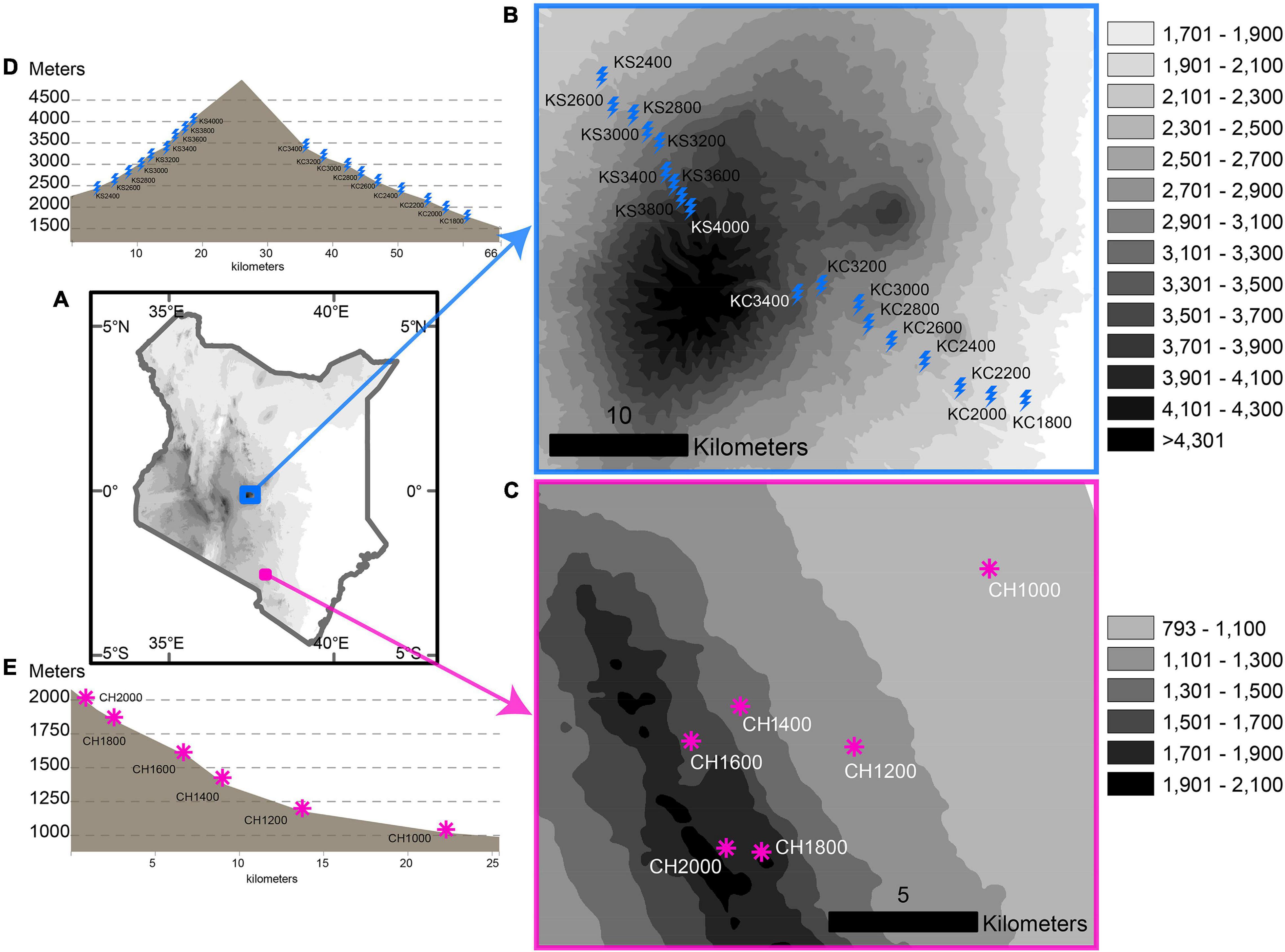
Figure 1. Study area and field sampling design of this study. (A) Map of Kenya showing the location of Mount Kenya and Chyulu; (B,C) Sampled elevational transects in Mt. Kenya and Chyulu, respectively. (D,E) Vertical elevational profile vs. distance along the Mt. Kenya and Chyulu transects, respectively.

The live-trapped animals were euthanized using chloroform after which the measurements of five external morphological traits (body mass in grams, head-body length, hind foot length, tail length, and ear length in centimeters) were recorded and the muscle and/or liver tissue extracted for later DNA analyses from all samples. Voucher specimens (skins and skulls) were also prepared for select specimens. The tissue samples and voucher specimens are deposited at the National Museums of Kenya, Nairobi, Kenya and Kunming Institute of Zoology, Kunming, China. All animal handling procedures adhered to the wildlife research laws of Kenya and the guidelines for the use of wild mammal species in research and education (Sikes and The Animal Care Use Committee of the American Society of Mammalogists, 2016). The research permit application was reviewed and approved by the Research and Ethics Committee of the Kenya Wildlife Service (permit number: KWS/BRM/5001).

Community Phylogenetic and Functional Characterization

For the input phylogenetic tree to estimate phylogenetic diversity indices, we used new sequences from this study to reconstruct a time-calibrated tree of all the unique gene pools (adopted as species units). For this, we extracted genomic DNA and sequenced the mitochondrial Cytochrome b gene from 1,142 samples. Recent evidence suggests Cytochrome b accurately reconstructs mammalian species’ ordinal, familial, and generic phylogenetic associations that match currently recognized relationships from molecular and morphological data (Tobe et al., 2010). First, total DNA was extracted from the muscle and/or liver tissue preserved at −80°C in 99.6% ethanol, using the sodium dodecyl sulfate method (Sambrook et al., 1989). A 1,140 base-pair region of the Cytochrome b gene was successfully amplified using polymerase chain reaction (PCR) with the primers L14724 (5′–GGACTTATGACATGAAAAATCATCGTTG–3′) and H14139 (5′–GATTCCCCATTTCTGGTTTACAAGAC–3′) (Kocher et al., 1989). The PCR conditions included denaturation at 95.0°C for 30 s, annealing at 59.0°C for 30 s, and extension at 72.0°C for 60 s for 40 cycles. The amplified products were sequenced in forward and reverse directions using the same primers, and the resulting chromatograms de novo assembled in Geneious Prime^® 2021.1.1² and aligned in Aliview based on the MUSCLE algorithm (Edgar, 2004; Larsson, 2014). The alignment was checked for internal stop codons and frameshifts in MEGA X (Kumar et al., 2018). From the 1,142 sequences, we identified 614 haplotypes using DnaSP V6.12.03 (Rozas et al., 2017). The haplotypes were retained as a new input alignment for reconstructing a preliminary phylogeny for species delimitation purposes (the haplotype data file was generated with sites with gaps or missing nucleotides and invariable sites included to retain the full 1,140 base-pair length). We also downloaded Cytochrome b sequences of the Numbat (Myrmecobius fasciatus), Brown-eared woolly opossum (Caluromys lanatus), and Water opossum (Chironectes minimus) from GenBank for use as an outgroup. For robustness and to check for topological inconsistencies of different phylogenetic methods, the preliminary phylogenetic tree was reconstructed using maximum likelihood in raxmlGUI 2.0 with 1,000 bootstrap replicates for branch support estimations (Stamatakis, 2014; Edler et al., 2021) and Bayesian inference in BEAST2 based on the uncorrelated lognormal clock and Yule speciation model with two MCMC runs each constituting 100 million MCMC chains sampled every 10 k runs and sampling convergence assessed in Tracer (Drummond and Rambaut, 2007; Bouckaert et al., 2019). In both analyses, we used the GTR + I + G4 nucleotide substitution model (identified as the best-fitting in ModelTest-NG v0.1.7; Darriba et al., 2019). We used the resulting trees and corresponding input alignments for species delimitation using tree- and distance-based methods capable of identifying common species units without prior sample assignment to taxonomic units. For the tree-based methods, we used the branch-cutting method (Ondřej, 2018), the multi-rate Poisson Tree Processes (mPTP) algorithm method (Kapli et al., 2017), and the single threshold general mixed Yule coalescent (GMYC) model (Fujisawa and Barraclough, 2013) while the distance-based method was implemented using assemble species by automatic partitioning (ASAP); (Puillandre et al., 2021).

The four delimitation methods differed in the number of OTUs estimated; ASAP yielded 49 OTUs, BCUT 49 OTUs, mPTP 58 OTUs, and GMYC 63 OTUs. The delimited OTUs were resolved into 63 clades, to capture all possible unique gene pools (populations or species); these were adopted as resembling currently recognized or potentially undescribed species pools (Supplementary Material 1). The clades’ nucleotide sequences were submitted to GenBank, accession numbers OL408896–OL408958. To assign species names to the clades, we cross-referenced our initial taxonomic assignments in the field, morphological characterizations, and BLAST search matches with the latest mammal checklists—Musser and Carleton (2005), Dieterlen (2013), Monadjem et al. (2015), Denys et al. (2017), and Musila et al. (2019b). Sequences corresponding to the 63 clades were used to reconstruct the final time-calibrated tree as an input for estimating phylogenetic diversity dimensions. Divergences were estimated based on the most recent common ancestor (MRCA) calibrations. Date estimates were extracted from Kumar et al. (2017) and the cited references. Consequently, we defined four calibration points: (i) the MRCA of subfamily Deomyinae and Gerbillinae (for clades under Acomys, Lophuromys, and Gerbilliscus genera) at 24.9 (interval: 17.0—32.8) mya, (ii) the MRCA of clades under the Muridae, Nesomyidae, and Gliridae family at 71 (interval: 66–75) mya, (iii) the MRCA of the Soricidae family clades (Crocidura, Sylvisorex, and Surdisorex genera) at 34 (23–45) mya, and (iv) the MRCA of the outgroup taxa (M. fasciatus, C. lanatus, and C. minimus)—Infraclass Metatheria—at 82 (interval: 74–89) mya. The tree was reconstructed in BEAST2 using lognormal priors, uncorrelated lognormal clock, and Yule speciation model, two 100 million generations-long MCMC runs sampled every 10,000 runs. The sampling adequacies were assessed in Tracer, the trees and log files combined in LogCombiner after discarding 10% as burn-in, and the combined trees summarized with the maximum clade credibility method in TreeAnnotator (Drummond and Rambaut, 2007). The phylogenetic trees may be seen in Supplementary Material 2.

The input data set for estimating functional diversity indices was compiled from several traits representing species morphological characterizations, diet, and activity patterns recorded in the field and from the published data sets. The morphology traits were taken from the measurements recorded in the field—adult body mass, length of head + body, tail, hindfoot, and ear (Supplementary Material 1). The measurements were represented in the final trait data set by the first two axes, which together explained 95.6% variance (PC1: 83.3%, PC2: 12.3%) following the transformation using principal component analysis (PCA). We obtained the data on diet and activity patterns from EltonTraits (Wilman et al., 2014), PHYLACINE (Faurby et al., 2018), and MammalDIET (Gainsbury et al., 2018). The resulting diet traits included the proportions composed of plants, fruits, nectar, seeds, invertebrates, mammals and birds, fish, reptiles and amphibians, and scavenging (Supplementary Material 1). Because the scaling of species traits varied between the different data sets, we used the first two axes of PCAs as final diet variables (Supplementary Material 1). We also used the activity traits from Wilman et al. (2014) represented by binary scores of three levels (nocturnal, diurnal, or crepuscular). Overall, the morphological, diet, and activity traits relate to species’ strategies of resource acquisition and usage underlying their life history and ecological strategies inherent in how biodiversity forms and is maintained in an area (Jones et al., 2009; Bohm et al., 2013). Functional diversity indices were estimated using the species-by-traits matrix or a functional trait dendrogram obtained by converting the matrix into a dendrogram of species relationships (Petchey and Gaston, 2002). The representation of species functional relationships using a dendrogram is easily applicable to and comparable with other biodiversity metrics using common frameworks, besides having a well-established historical background (Jarzyna and Jetz, 2016).

Compilation of Potential Abiotic Predictors

The environmental predictor data were extracted from publicly available repositories or following data requests from authors. To test the water-energy availability hypothesis, we used annual mean precipitation (PAM), annual precipitation seasonality (PAS), annual mean temperature (TAM), annual temperature seasonality (TAS), and annual actual evapotranspiration (AET). We obtained TAM and TAS data for the near current climate data from the bioclimatic variables database (Fick and Hijmans, 2017), downloaded from https://www.worldclim.org/data/index.html. The AET data were extracted from Running et al. (2019); to control for anomalies associated with uneven monthly and yearly trends, we extracted 11 yearly AET products spanning 2009–2019 and averaged them into a single layer using the Raster Calculator tool in ArcMap. The AET was downloaded using the Application for Extracting and Exploring Analysis Ready Samples (AρρEEARS) (AppEEARS Team, 2020). To test the primary productivity hypothesis, we used normalized difference vegetation index (NDVI) and vegetation characterization (VEG). The NDVI data were extracted as the spectral index of vegetation reflectance in the near-infrared and red electromagnetic spectrum portions from Didan (2015), downloaded using AρρEEARS. For vegetation characterization data (VEG), we consolidated field-observed vegetation types [see Table 1 in Musila et al., 2019a and vegetation classification data from the potential natural vegetation map of eastern Africa (extract for Kenya) (van Breugel et al., 2015)].³ The topographic heterogeneity hypothesis was explored using elevation (ELEV) and terrain ruggedness index (TRI). The ELEV data were obtained from the NASA Shuttle Radar Topography Mission 1 arc second data downloaded using AρρEEARS. Then, the TRI was derived from the ELEV layer using the Raster analysis “Terrain Ruggedness Index” function in QGIS (QGIS Development Team, 2021).

Estimation of Phylogenetic and Functional Indices

The increasing realization that species richness (SR) poorly surrogates functional and phylogenetic biodiversity dimensions, especially when life history and geographical specificities are factored, has led to increased adoption of phylogenetic and functional dimensions in the biodiversity field as a more holistic appraisal of conservation gaps and ecological restoration needs (Chao et al., 2014; Mazel et al., 2014; Tucker et al., 2017). We estimated six diversity indices representing the phylogenetic and functional sum of difference among observations—phylogenetic richness (PD) and functional richness (FD), average divergence among observations—phylogenetic mean nearest taxon distance (PD^MNTD) and functional mean nearest taxon distance (FD^MNTD), and variances of differences among observations (community structure)—phylogenetic nearest taxon index (PD^NTI) and functional nearest taxon index (FD^NTI). This approach ensured a more holistic characterization of the sampled sites. Because the PD and FD rely on species (taxonomic identities) distributions across functional and phylogenetic spaces, they are inherently correlated with species richness (Pavoine et al., 2013). On the other hand, the MNTD and NTI indices control for species richness non-independence by comparing observations to null model communities. Overall, these indices are broadly popular in the literature, which enhance the comparability of our results (Chao et al., 2014; Tucker et al., 2017).

For these implementations, the number of samples per clade (abundances) were first normalized using the Hellinger transformation (Legendre and Gallagher, 2001), which standardized the recorded clade numbers to sample totals by converting the absolute values to relative values. The transformation is suitable for species abundances as it gives low weights to variables with low counts and many zeros (Legendre and Gallagher, 2001). The three input data sets (site-by-clade community composition, phylogeny, and traits) and those of predictors were then sorted to match using the functions match.phylo.comm and match.phylo.data in R package picante (Kembel et al., 2010) and the all.equal function in the base package (R Core Team, 2021). The PD and FD were computed using the ses.fd function of picante with the phylogeny and functional dendrogram as the corresponding tree inputs. The PD^MNTD was estimated as the abundance-weighted estimates of evolutionary (phylogenetic) diversity using the ses.mntd function (Webb et al., 2002; Webb and Donoghue, 2005) in picante. Higher PD^MNTD values indicate that the sampled community is comprised of less related taxa. The FD^MNTD was estimated analogously as PD^MNTD after substituting the phylogenetic tree with the functional traits’ dendrogram (Webb et al., 2002, 2008). The PD^NTI and FD^NTI represented the phylogenetic and functional community structure, respectively, with significantly positive values suggesting that communities are comprised of taxa that are more closely related than expected by chance while negative values suggest that communities are comprised of taxa that are less closely related than expected by chance. They were estimated from the standardized effect size of PD^MNTD and FD^MNTD by comparing with null-community expectations. The null communities were generated using 9,999 randomizations through 1,000 iterations based on the name-shuffling null model, which shuffles species names across the phylogenetic tree and the functional dendrogram/species-by-trait matrix. The resulting values were multiplied by − 1 (negative 1) to translate them to PD^NTI and FD^NTI (Webb et al., 2008). The number of taxa that were also output from the above estimations was used to represent SR and explore correlations between the indices.

Multivariate Analysis

To align the predictors that were obtained as raster layers—PAM, PAS, TAM, TAS, AET, NDVI, ELEV, and TRI, we resampled (bilinear interpolation) them to a common 0.00277778 × 0.00277778-degree cell size using SDMtoolbox 2.0 in ArcMap (ESRI, 2011; Brown et al., 2017). We then extracted variables per sample using the Point sampling tool in QGIS and log-transformed the resulting values to normalize distributions (remove distribution skewness). To handle potential statistical and inferential issues associated with high multicollinearity (Graham, 2003), we retained single predictors from highly correlated sets [Pearson’s r | > 0.7| (Dormann et al., 2013)]. We further used the variance inflation factor (VIF) analysis to handle overall predictors’ non-independence, which might inflate standard errors when building regression models. For this, we used the generalized linear model (GLM), with the predictors as explanatory (independent) variables and each diversity index as response (dependent) variables. We used a VIF cut-off of three “3” (Zuur et al., 2010) at which predictors with VIFs greater than the cut-off were dropped, VIFs recalculated, and the procedure repeated until all predictors achieved the cut-off threshold. We used the glmulti R package (Calcagno, 2019) to find the best combination of predictors explaining diversity trends from all possible combinations of predictors, using main effects and the exhaustive screening option ranked by Akaike information criterion (AIC) scores. In several cases, there were more than one top best-fit models, which were not clearly distinguished from the top best model. Therefore, we averaged all models with changes in AIC scores (AIC^Δ) < 2 (Burnham and Anderson, 2004) using the R package MuMIn (Barton, 2019). The final global models were fitted with GLM and generalized additive model (GAM), which were preferred for providing data multidimensionality and non-linearity, as is characteristic of ecological relationships, with GAM concurrently used to automate the detection and estimation of non-linear effects (Hastie and Tibshirani, 1990; Guisan et al., 2002). The GLMs were fitted using the stats R base package (R Core Team, 2021) while GAMs were fitted using the mgcv R package with the thin plate regression splines (Wood, 2011). Because the responses (diversity indices) and explanatory variables (predictors) fitted normal distributions well, both models were fitted using the Gaussian probability distribution family and linear “identity” link. The proportions of diversity indices explained by the models and the relative importance of each predictor were estimated from the adjusted r-squared (r²_a) and model coefficient. The bivariate correlations between predictors systematically differed between sites and slopes (Supplementary Material 3); therefore, analyses were implemented separately for the three elevational slopes (Chogoria, Sirimon, and Chyulu), and the contiguous Mt. Kenya data set (combining Chogoria and Sirimon). Consequently, we used 24 GLM and GAM models, each for the 6 diversity indices, with a similar number of models used to explore the individual predictive influence of elevation and vegetation on diversity variances.

Results

Overview of Sampling and Diversity Distributions

The sample-size- (abundance-) based rarefaction and extrapolation curves of species sampling showed that transect sampling achieved asymptotes for all Hill diversity indices (Supplementary Material 4). The phylogenetic analyses recovered well-resolved associations at both deep and terminal divergences, with ordinal and familial relations matching currently recognized mammalian taxonomies (Supplementary Material 2). The samples were classified into 2 orders—Rodentia and Eulipotyphla, 4 families—Gliridae, Muridae, Nesomyidae, and Soricidae, 20 genera, and 63 clades (adopted as species units in the current study but not necessarily corresponding to currently recognized species) (Supplementary Material 1). Of the total 63 clades, 34 clades were represented in Mt. Kenya (31 clades in Chogoria and 23 clades in Sirimon) and 30 clades were represented in Chyulu.

On average, Chyulu was phylogenetically (PD) (333.3 ± 91.9 vs. 307.4 ± 78.3) and functionally (FD) (1.04 ± 0.28 vs. 1.01 ± 0.28) richer than Mt. Kenya. However, Mt. Kenya had a higher PD^MNTD (83.75 ± 23.54 vs. 61.8 ± 24.21) and FD^MNTD (0.255 ± 0.089 vs. 0.161 ± 0.075) compared to Chyulu. The PD^NTI and FD^NTI were both negative in Mt. Kenya (− 0.29 ± 0.94 and − 0.114 ± 0.0838, respectively) but positive in Chyulu (0.642 ± 1.102 and 0.75 ± 0.787, respectively) on average. Although fewer clades were represented in Sirimon, it had averagely higher PD and FD than Chogoria (317.71 ± 84.96 vs. 296.32 ± 69.75 and 1.063 ± 0.276 vs. 0.952 ± 0.285, respectively). Similarly, the PD^MNTD and FD^MNTD were also higher in Sirimon than in Chogoria (89.42 ± 20.52 vs. 77.67 ± 25.25 and 0.279 ± 0.082 vs. 0.231 ± 0.09, respectively). The PD^NTI and FD^NTI were both averagely negative in Sirimon (− 0.613 ± 0.857 and − 0.369 ± 0.723) but positive in Chogoria (0.057 ± 0.909 and 0.158 ± 0.875).

Associations between diversity indices were congruous between elevational gradients. The PD and FD increased with increasing SR while PD^MNTD and FD^MNTD decreased with increasing SR, all with statistically significant effects (Supplementary Material 5). On the other hand, PD^NTI and FD^NTI were not statistically significantly associated with SR, with PD^NTI increasing in Chyulu and Chogoria but decreasing in Sirimon as SR increased while FD^NTI decreased in Sirimon and Chogoria but increased in Chyulu as SR increased (Supplementary Material 5).

Phylogenetic and Functional Diversity Along Elevational Gradients

The predictive influence of elevation on diversity variances was observably not any better than that of the environmental variables retained in the best models or vegetation (Table 1). The strongest influence, based on the proportion of variance explained (r²_a) was in Mt. Kenya (0.193) followed by Chogoria (0.095), Chyulu (0.0445), and the weakest in Sirimon (0.016). Between the indices, the strongest influence was on FD (r²_a = 0.112) followed by PD^MNTD, PD, PD^NTI, FD^MNTD, and the weakest on FD^NTI (r²_a = 0.066) (Table 1).

TABLE 1

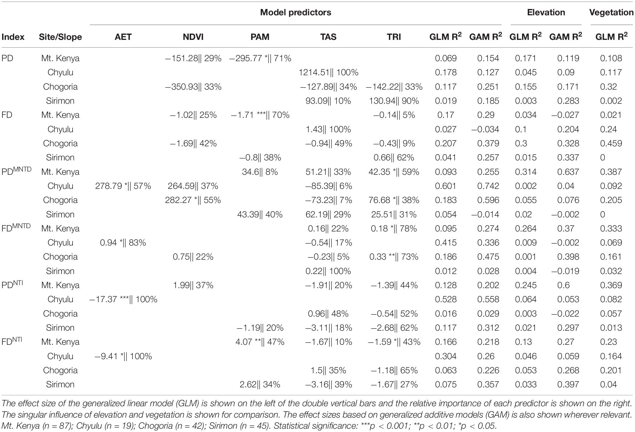
Table 1. Summary of best-fit model coefficients across diversity indices and sites.

The richness indices (PD and FD) were positively associated with elevation in Mt. Kenya, where they portrayed a unimodal hump-shaped curve—mid-elevation peak—around 3300 m in the former (Figure 2 and Table 2). Between the Mt. Kenya slopes, the PD and FD increased in Chogoria up to around 2,800 m and then declined, while in Sirimon both the indices non-significantly declined multimodally; with the two curves combining into the hump-shaped curve in Mt. Kenya (Figure 2). Both PD and FD unimodally increased with elevation in Chyulu, with no well-defined peaking around mid-elevations (Figure 2 and Table 2).

FIGURE 2

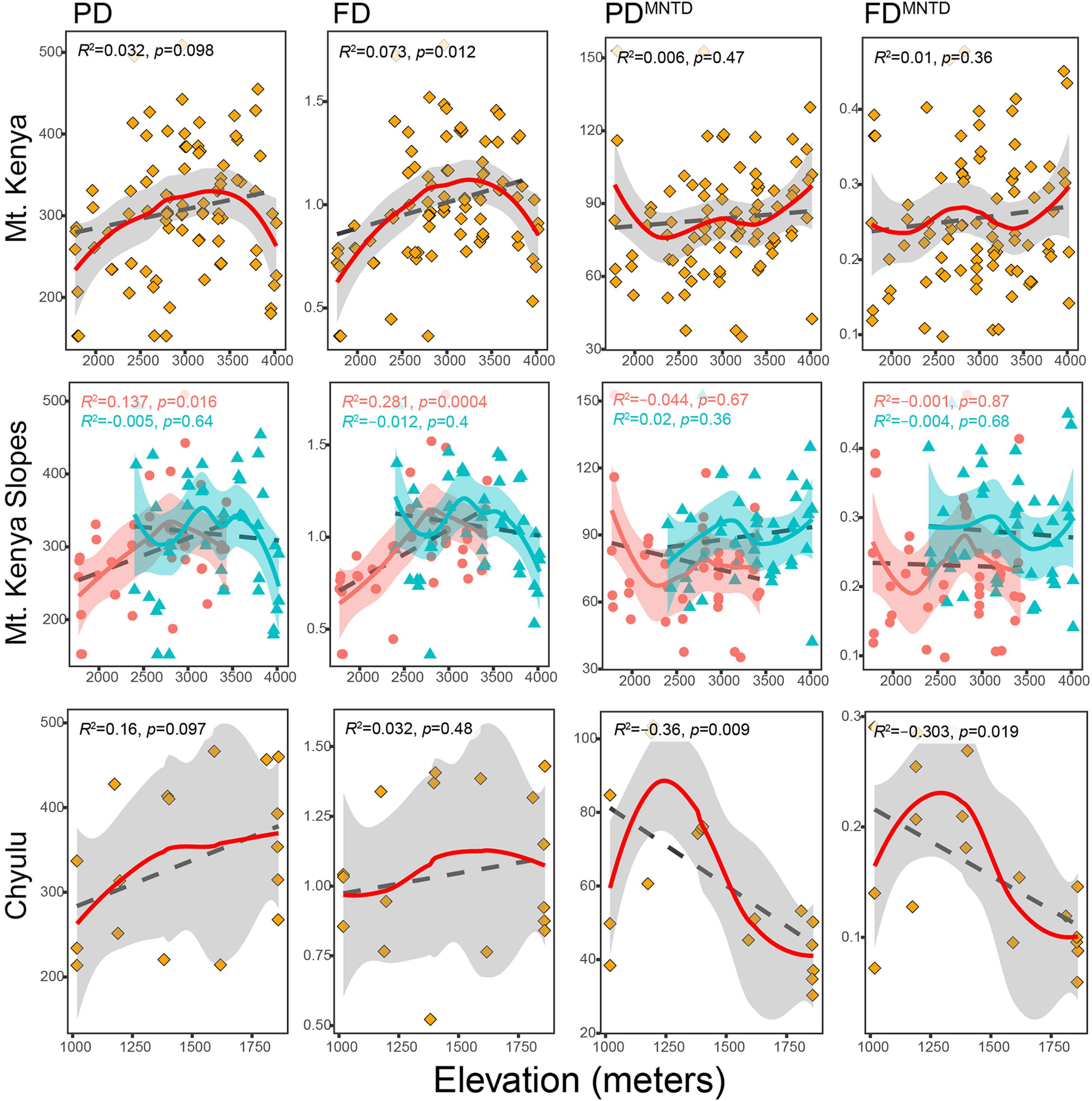
Figure 2. The distribution of phylogenetic and functional diversity and divergence indices (y-axes) along elevational gradients (x-axes) between the sites and indices. Points represent traplines and lines represent regression lines—local polynomial (solid colored lines) and generalized linear model (GLM; black dashed lines). In the Mt. Kenya plots, light red-colored dots represent Chogoria traplines while the dark shade of cyan triangular points represents Sirimon traplines.

TABLE 2

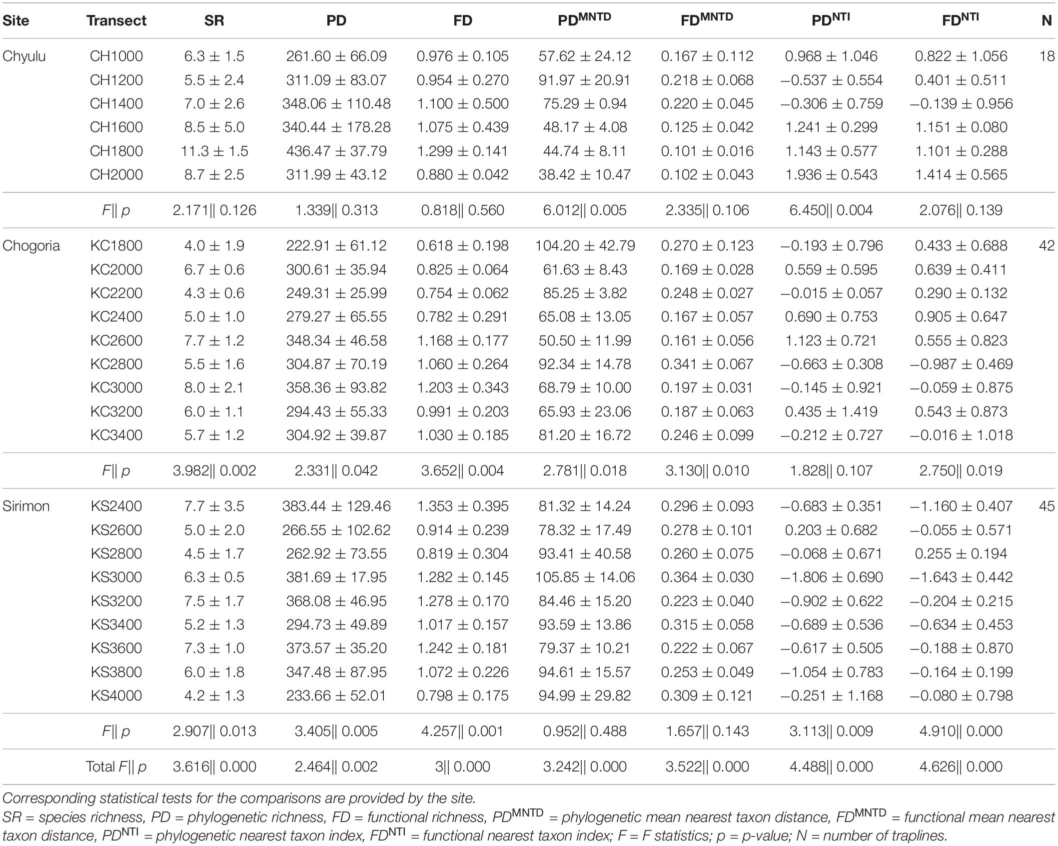
Table 2. Summary statistics of diversity indices between the transects.

The divergence indices (PD^MNTD and FD^MNTD) portrayed weaker elevational trends—near-horizontal response curves—compared to PD and FD in Mt. Kenya unlike in Chyulu (Figure 2). In Mt. Kenya, PD^MNTD and FD^MNTD increased with elevation, although non-significantly, indicating that phylogenetic and functional relationships between clades declined toward upper elevations overall. In contrast, different divergence trends were observed in Sirimon and Chogoria where both the indices decreased with elevation except for FD^MNTD in Sirimon. Both PD^MNTD and FD^MNTD declined statistically significantly with elevation in Chyulu (Figure 2 and Table 2).

The community structure indices (PD^NTI and FD^NTI) also showed weak associations with elevation, with p > 0.05 except for PD^NTI in Mt. Kenya and Chyulu (Figure 3A). Both PD^NTI and FD^NTI declined with increasing elevation in Mt. Kenya, Chogoria, and Sirimon but increased in Chyulu and Sirimon (FD^NTI only) (Figure 3A). Thus, the tendency of assemblages to be phylogenetically and functionally overdispersed (less closely related than expected by chance) increased with elevation in Mt. Kenya while clustering (more closely related than expected by chance) increased with elevation in Chyulu (Figure 3B). Overall, assemblages were randomly phylogenetically and functionally structured (of 105 traplines, 98 had PD^NTI with p > 0.05 and 103 for FD^NTI).

FIGURE 3

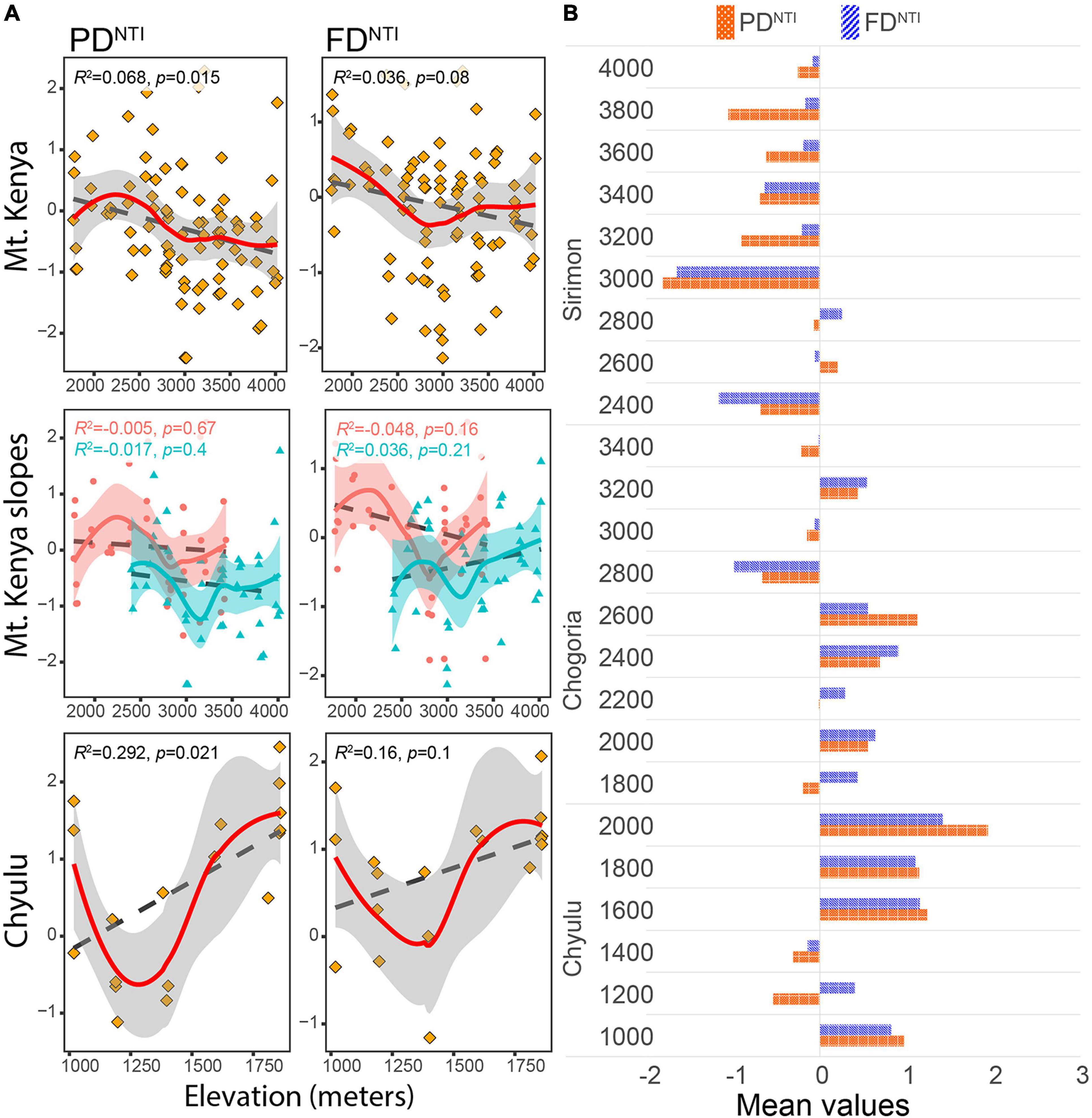
Figure 3. The distribution of phylogenetic and functional community structure indices along elevational gradients in Mt. Kenya and the Chyulu Hills. (A) The association of community structure (y-axes) with elevation (x-axes) between elevational gradients. (B) The distribution of mean structure indices between the transects. Points represent traplines and lines represent the local polynomial (colored continuous lines) and GLM (black dashed line) regression lines. In the Mt. Kenya plots, light red-colored dots represent Chogoria traplines while the dark shade of cyan triangular points represents Sirimon traplines.

Environmental Predictors of Diversity Variances

Only four predictors were retained across the best models; annual mean precipitation (PAM), temperature seasonality (TAS), annual actual evapotranspiration (AET), normalized difference vegetation index (NDVI), and terrain ruggedness index (TRI) (Figure 4A and Table 1). The proportions of diversity variances accounted for by the best models (r²_a) differed between the sites and indices, averaging 0.161 (0.096 − 0.233) and the highest in Chyulu (0.342) followed by Chogoria (0.129), Mt. Kenya (0.12), and the least in Sirimon (0.053) (Figure 4B and Table 1). Observably, no single index was consistently similarly explained (Figure 4A and Table 1). Also, the GAMs were notably consistently better at explaining associations than GLMs (Figure 4B and Table 1).

FIGURE 4

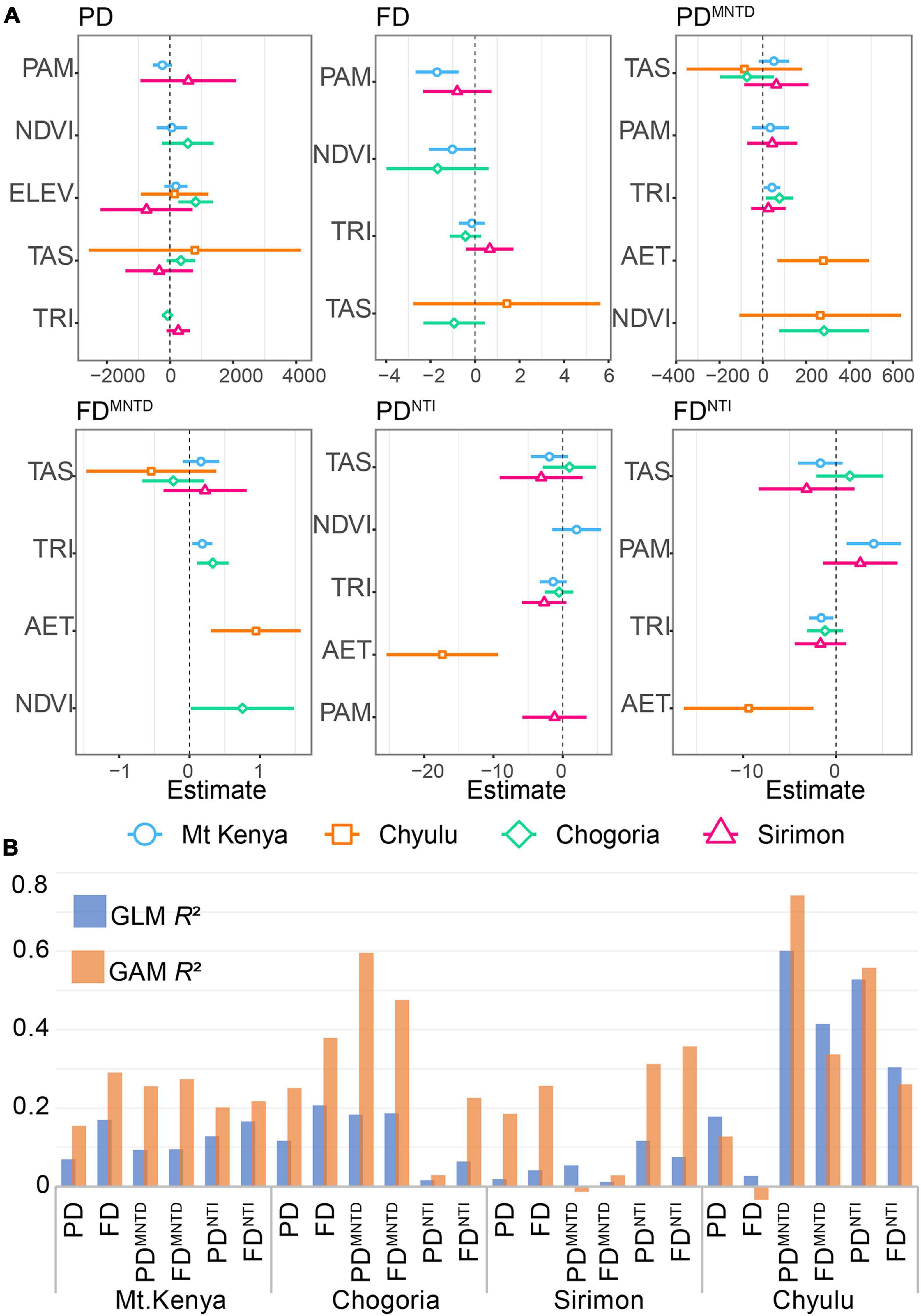
Figure 4. The regression coefficients of association between diversity variances and environmental predictors. (A) Plots of regression coefficients summarizing the association between predictors and indices between the sites. (B) The proportion of diversity variances accounted for by the combination of predictors retained in the best-fit models.

The response curves of associations between diversity variances and the strongest predictors across the sites and indices are illustrated in Supplementary Material 6. In Mt. Kenya, annual mean precipitation (PAM) and terrain ruggedness index (TRI) were the most important predictors. The PAM explained the biggest relative proportion of the r²_a in PD, FD, and FD^NTI while TRI accounted for the biggest proportion of the PD^MNTD, FD^MNTD, and PD^NTI variances (Figure 4A and Table 1). Notably, the most important predictors in Chogoria and Sirimon differed from those of Mt. Kenya, with TAS, NDVI, and TRI as the strongest predictors (Table 1). In Chogoria, the lowest r²_a, which was in PD^NTI (r²_a = 0.016), was explained mostly by TRI, followed by FD^NTI (r²_a = 0.063) which was also explained mostly by TRI, PD (r²_a = 0.117) by annual temperature seasonality (TAS), PD^MNTD (r²_a = 0.183) by the normalized difference vegetation index (NDVI), FD^MNTD (r²_a = 0.186) by TRI, and the highest in FD (r²_a = 0.207) which was mostly correlated with TAS. On the other hand, the explained diversity variances in Sirimon ranged between 0.012 and 0.117 and were mostly correlated with PAM, TAS, and TRI. The PAM was the strongest predictor of the 0.054 r²_a of PD^MNTD with TAS explaining most of the 0.012 r²_a of FD^MNTD and 0.075 r²_a of FD^NTI and TRI explaining most of the 0.019 r²_a of PD, 0.041 r²_a of FD, and 0.117 r²_a of PD^NTI (Figure 4B and Table 1). In Chyulu, AET and TAS were the strongest predictors of the 0.027–0.601 r²_a across the indices. The AET explained most of the 0.601 r²_a of PD^MNTD, 0.415 r²_a of FD^MNTD, 0.528 r²_a of PD^NTI, and 0.26 r²_a of FD^NTI while TAS accounted for most of the 0.178 r²_a of PD and 0.027 r²_a of FD (Figure 4B and Table 1).

Despite the relatively well-variegated vegetation distribution along elevational gradients (Supplementary Material 7), its singular influence on diversity variances remained low (Table 1). The r²_a of vegetation ranged between 0 and 0.459 across the sites and indices (Table 1). Across the indices, the highest r²_a was in Mt. Kenya (0.241), followed by Chogoria (0.234), Chyulu (0.127), and the least in Sirimon (0.014). The influence of vegetation among the indices did not greatly differ, with the r²_a range of 0.13–0.18; being the strongest for FD and the weakest for PD^NTI (Table 1).

Discussion

The Afrotropical realm holds the highest mammal diversities globally, which are also most at the risk of extinction (Ceballos and Ehrlich, 2006; Jenkins et al., 2013; Raven et al., 2020). However, there are very few studies on local-scale ecosystem species mechanisms, such as elevational patterns in ecologies and evolutionary histories, with hardly any studies based on phylogenetic and functional dimensions. Here, we sought to answer the two main questions inherent in understanding mammal-environment feedbacks—what are the patterns of small mammal phylogenetic and functional diversity and community structure along elevational gradients and what are the main environmental predictors of small mammal phylogenetic and functional diversity and community structure along elevational gradients? Based on a comprehensive elevational sampling of Mt. Kenya and the Chuylu Hills mountain range, our analyses offer a first-of-its-kind insight into how the phylogenetic and functional diversity of small mammals vary along tropical mountain elevational gradients and how patterns are associated with environmental predictors.

Our first aim was to untangle the phylogenetic and functional diversity and community structure trends along the elevational gradients of Mt. Kenya and the Chyulu Hills and draw comparisons with species richness (SR), which has dominated the literature on diversity-elevation associations. We observed a hump-shaped PD and FD association as elevation increased in Mt. Kenya (combining the Chogoria and Sirimon slopes), with Chogoria portraying a nearly similar curve. On the other hand, in Sirimon, the PD and FD were multimodally associated with elevation with no definite peak(s) while in Chyulu, the PD and FD unimodally increased with elevation. While the Mt. Kenya and Chogoria trends conform to a typical SR distribution in tropical mountains (McCain and Grytnes, 2010), the differing trends observed in Sirimon and Chyulu trends have also been recorded. In an affiliated Mt. Kenya study, Musila et al. (2019a) observed the highest number of small mammals’ species around mid-high elevations in Chogoria but little elevational variation in Sirimon. Due to a high correlation of SR with PD and FD (Supplementary Material 5), the hump-shaped PD and FD association with elevation can be considered to be well supported by previous studies of mammalian assembling in tropical mountains (Rahbek, 1995; McCain, 2005; Chen et al., 2017; Shuai et al., 2017). Notably, however, these results contrast the Dreiss et al. (2015) study of neotropical rodents, the PD and FD declined monotonically as elevation increased. Also, Dehling et al. (2014) observed functional richness and phylogenetic diversity decreased monotonically with increasing elevation in the Andes while Zhou et al. (2019) study of phylogenetic and functional diversity of the Mt. Kenya seed plants was also dominated by PD and FD declines as elevation increased. These contrasting observations highlight the potential impacts of context-specific differences (animal group, mountain locality, or elevational gradient), which are even evident in the slope-wise—Chogoria vs. Sirimon—abiotic characterization (Figure 5). Although mid-elevation peaking in the PD and FD (as a surrogate of SR) can dominate low-altitude mountains in vertebrate assemblages (Nogués-Bravo et al., 2008; Weier et al., 2016; Quintero and Jetz, 2018), the trends observed here in Chyulu imply that these low elevation highlands portray a broader array of diversity-elevation patterns. Also, the Chyulu Hills has much gentler slopes with broader and less definite base elevations and an overall harsher environment as most transects are characterized as arid and semiarid, which eliminates the formation of distinct mountain fauna for elevational trends. Studies generalizing elevation-diversity associations should also note environmental characterizations of the mountains for greater insights into local assembly dynamics in small mammal communities.

FIGURE 5

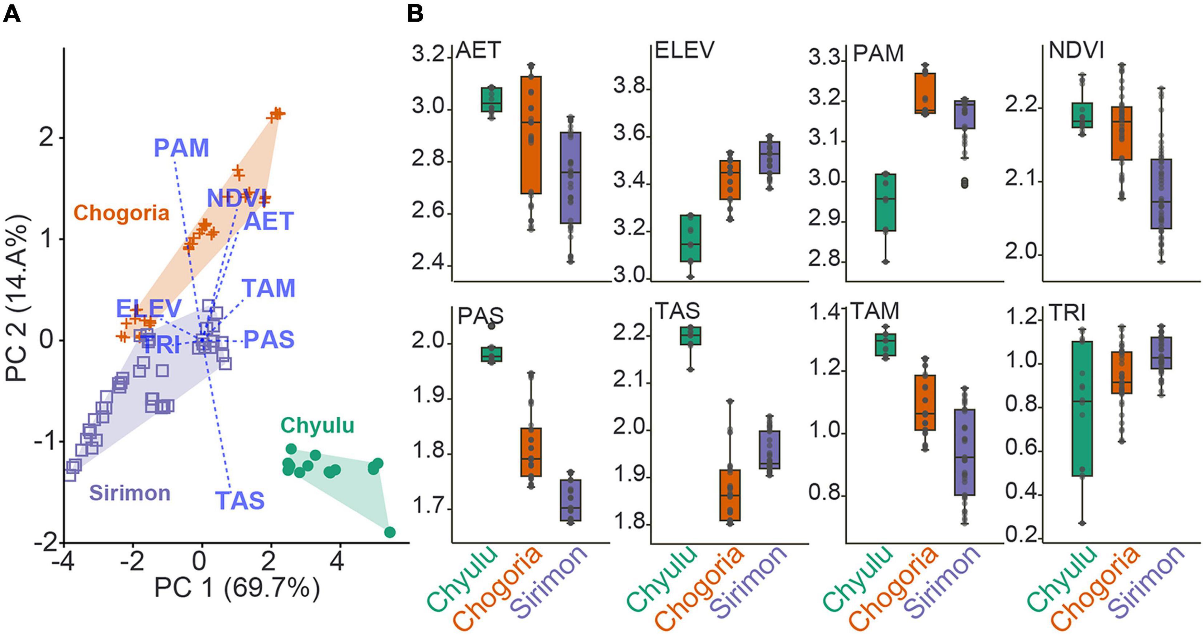
Figure 5. The environmental characterization of Mt. Kenya and Chyulu based on the predictors used in the study. (A) Scatter plot of the first two principal component analysis (PCA) axes illustrating differences between elevational gradients. (B) Boxplots comparing individual predictor averages between the sites.

The increase of PD^MNTD and FD^MNTD with elevation in Mt. Kenya, Chogoria, and Sirimon relays a tendency of decreasing phylogenetic and functional affinity with increasing elevation. Such patterns are commonly attributed to the harsher habitats at higher elevations (such as night-freezing temperatures and resource-poor conditions in Mt. Kenya), which depress speciation and generational turnover for most small mammals, in the process, leading to the persistence of a few taxa uniquely adapted species (Hawkins et al., 2003; Graham et al., 2014). The clades sampled at the highest elevations in Mt. Kenya, besides the locally abundant ones such as clades in the genera Lophuromys and Crocidura (Musila et al., 2019a; Onditi et al., 2021), included Dendromus, Otomys, Dasymys, and Rhabdomys clades that were overall rarer at transects in lower elevations (Supplementary Materials 1, 4) and noted to have evolved to prefer the moist highland forests (Carleton and Musser, 2013; Denys et al., 2017). In Chyulu, such specialists included clades in the genera Grammomys, Otomys, Praomys, and Zelotomys, which were not recorded below the 1,800- and 2,000-m transects that had patches of Afromontane rainforests. These clades are only known from humid habitats, including highland forests, forest edges, and swamps (Monadjem et al., 2015; Denys et al., 2017; Musila et al., 2019b). The narrow transect ranges they were recorded in this study suggest they might be occurring in much narrower elevational ranges than is currently recorded, leading to pronounced influences on the phylogenetic and functional trends along elevational gradients. In Chyulu, PD^MNTD and FD^MNTD steeply declined as elevation increased, this can be attributed to higher elevational transects comprising more species that are closely related, i.e., forest-dependent clades cited above, compared to the lower elevational transects, which were dominated by a few clades that are common in more arid habitats—Acomys (not recorded above 1,600 m) and Gerbilliscus (not recorded above 1,600 m). This is also supported by a significant increase in PD^NTI with elevation, supporting that the likelihood of assemblages being clustered (comprised of the clades that are phylogenetically more related than expected by chance) increased with decreasing elevation. Such patterns typically manifest the influence of strong environmental filtering (Webb, 2000), which herein reflects the less productive habitats (Somalia-Masai Acacia-Commiphora bushlands and thickets and dry combretum wooded grasslands) that dominated the 1,200- and 1,000-m transects. The non-significant deviations of PD^NTI and FD^NTI from null models appear common when these indices are estimated from the standardized effect size of taxon distances across mammal, avian, herptile, and floral studies (Cisneros et al., 2014; Dehling et al., 2014; Dreiss et al., 2015; Meza-Joya and Torres, 2016; Zhou et al., 2019; Montaño-Centellas et al., 2020).

Our second main question pertained to the environmental predictors of small mammal phylogenetic and functional diversity and community structure along elevational gradients. Here, we tested three main hypotheses (water-energy availability, primary productivity, and topographic heterogeneity) implicated in the literature as strong mammal diversity drivers in tropical ecosystems (Hawkins et al., 2003; McCain, 2005; McCain and Grytnes, 2010). Considering the retention of AET, PAM, and TAS as the most important predictors of diversity variances across most of the models, our results notably strongly support the water-energy availability hypotheses (Rosenzweig, 1992; Rahbek, 1995) (Figure 4 and Table 1). These predictors represent access to water resources, which are major limiting factors for mammals, especially in warmer tropical climates (Hawkins et al., 2003), and their importance as a key diversity and assembly predictor in Mt. Kenya conforms to these influences. Temperature and precipitation are also strong diversity drivers in other vertebrate and floral groups (Kessler and Kluge, 2008; Hanz et al., 2019; Ramirez-Bautista and Williams, 2019; Zhou et al., 2019; Rowan et al., 2020), African mammal communities (Kamilar et al., 2014, 2015), and plant–animal diversity and interactions in Mt. Kilimanjaro (Schellenberger Costa et al., 2017; Albrecht et al., 2018), as observed here for small mammals. Notably, AET and TAS were retained as strongly correlated with diversity variances mostly in Chyulu (Table 1), suggesting that their influence on small mammal assembling might be stronger in dominantly less moist habitats. The Chyulu Hills and Mt. Kenya are well differentiated based on the predictors, with Chogoria and Sirimon also observably differing for some predictors (Figure 5 and Supplementary Material 3). The Mt. Kenya–Chyulu differences are supported by the previous studies that observed higher diversity variances explained by environmental variables in less productive/harsher ecosystems (Schluter and Pennell, 2017; Harvey et al., 2020), with harshness interpreted as higher TAS and PAS and lower PAM and AET. On the other hand, the Chogoria-Sirimon contrasts probably relate to aspect-wise variations in precipitation and temperature of tropical mountains, which has been observed to be strongly associated with small mammal diversity distributions in tropical mountains (McCain, 2007; Curran et al., 2012; Weier et al., 2016).

Although our results suggest that the habitat productivity hypothesis (Rosenzweig, 1992; McCain et al., 2018) might be a weaker predictor of PD and FD variances along elevational gradients in the tropics, the AET, PAM, and TAS control of primary habitat productivity, in terms of vegetation diversity and abundance (Hawkins et al., 2003), which has more direct influences on small mammal ecological strategies and the association may confound the predictive influence of NDVI and vegetation types on diversity variances. Notably, the retention of TRI as the strongest contributor to model-explained diversity variances in 9 of the 24 models supports the topographic heterogeneity hypothesis (Rosenzweig, 1995) as a strong regulator of how species assemble and interact based on their phylogenetic and functional characterizations in tropical mountains. Despite a few studies focusing on TRI’s association with vertebrate elevational diversity trends on Afrotropical mountains, topographic heterogeneity at local habitat level scales is a significant regulator of primary habitat diversity and productivity (Stein and Kreft, 2015). This pertains to TRI and elevation being intrinsic regulators of animal ecologies through a direct manipulation of animal movement and occurrence, niche dimensions, and vegetation heterogeneity, which, in the process, drive predator–prey relationships, species behavior, and phenotypic trait functions (Whittaker et al., 1973). Also, TRI and elevation control vegetational compositional heterogeneity, where higher and more rugged terrains have more diverse and richer habitats in terms of vegetation resources leading to corresponding higher diversity of mammals (Kerr and Packer, 1997; Yasuhiro et al., 2004; Rahbek et al., 2019b).

Notably, some fundamental caveats must be considered in interpreting and/or applying our findings. Because community ecology studies based on primary sampling assume fair sampling of all resident fauna, imperfect sampling is common, while site conditions such as geographical accessibility and weather conditions can also hinder appropriate sampling. Although the Cytochrome b gene provided a well-resolved informative and resolved topology of species associations with deep and terminal divergences well supported by the latest species accounts, congruous with recent observations, these associations must be interpreted within the phylogenetic limitations of Cytochrome b for mammalian groups (Tobe et al., 2010). The elevational gradient diversity patterns appear to distinctly vary according to the sampling strategy, i.e., whether the data set covered a single slope or averaged multiple elevational gradient slopes. Future mammal surveys on the Chyulu Hills should employ multi-slope transects to establish with certainty the absence or presence of a mid-elevation richness or diversity peak.

Conclusion

We explored the distribution of various phylogenetic and functional diversity indices along elevational gradients of Mt. Kenya and the Chyulu Hills, the two contrasting montane systems, but typical of Afromontane ecosystems. We then tested the associations between the diversity indices and several potential environmental predictors how they relate to the diversity distributions. The association of diversity indices with elevation varied between Mt. Kenya and Chyulu and even between the Mt. Kenya slopes (Chogoria and Sirimon). The phylogenetic and functional richness peaked around mid-elevations in Mt. Kenya, unimodally increased or decreased in Chogoria and Sirimon, and monotonically increased in Chyulu. On the other hand, the divergence and community structure indices were relatively weakly associated with elevation. The tendency of assemblages to be phylogenetically and functionally more closely related than expected by chance decreased with elevation in Mt. Kenya but increased in Chyulu. The annual mean precipitation, temperature seasonality, actual evapotranspiration, and terrain ruggedness were the strongest predictors between the sites and indices. These results provide a holistic understanding of small mammal phylogenetic and functional diversity and assembly patterns, with vital conservation implications. For instance, while Sirimon had fewer clades compared to Chogoria and Chyulu, and even the contiguous Mt. Kenya community (Chogoria and Chyulu), it had the higher phylogenetic and functional richness (PD and FD) and divergence (PD^MNTD and FD^MNTD), on average. As such, biodiversity prioritization based on species richness alone would neglect the high evolutionary and feature diversity in Sirimon, in the processes, threatening the ecological stability of the Mt. Kenya ecosystem. These slope-wise diversity distributions and associations with abiotic predictors highlight the need for more local-scale habitat level ecological and evolutionary studies, especially in the Afromontane highlands where there has hardly been any progress in local-scale studies based on the phylogenetic and functional diversities.

Data Availability Statement

The raw data supporting the conclusions of this article will be made available by the authors, without undue reservation.

Ethics Statement

This study was reviewed and approved by the Research and Ethics Committee of the Kenya Wildlife Service (permit number: KWS/BRM/5001).

Author Contributions

KO, W-YS, X-YL, and X-LJ conceptualized and designed the study. KO, W-YS, X-YL, Z-ZC, QL, SM, EK, and X-LJ conducted fieldwork and contributed to the study design. KO and S-WH performed the lab work. KO wrote the first draft of the manuscript. All authors contributed to consequent revisions of the manuscript and approved the final version for submission.

Funding

This study was supported by the Sino-Africa Joint Research Centre, Chinese Academy of Sciences (SAJC202103). KO was sponsored by the CAS-TWAS President’s Fellowship Program.

Conflict of Interest

The authors declare that the research was conducted in the absence of any commercial or financial relationships that could be construed as a potential conflict of interest.

Publisher’s Note

All claims expressed in this article are solely those of the authors and do not necessarily represent those of their affiliated organizations, or those of the publisher, the editors and the reviewers. Any product that may be evaluated in this article, or claim that may be made by its manufacturer, is not guaranteed or endorsed by the publisher.

Acknowledgments

We are grateful to the Kenya Wildlife Service and Kenya Forest Service offices for granting permit to the study areas, and for providing security and logistical support in the field. We also thank the personnel of the Zoology Department and the Mammalogy Section at the National Museums of Kenya for facilitating operations in the field and joining forces in field surveys.

Supplementary Material

The Supplementary Material for this article can be found online at: https://www.frontiersin.org/articles/10.3389/fevo.2021.742524/full#supplementary-material

Footnotes

References

Albrecht, J., Classen, A., Vollstädt, M. G. R., Mayr, A., Mollel, N. P., Schellenberger Costa, D., et al. (2018). Plant and animal functional diversity drive mutualistic network assembly across an elevational gradient. Nat. Commun. 9:3177. doi: 10.1038/s41467-018-05610-w

PubMed Abstract | CrossRef Full Text | Google Scholar

AppEEARS Team (2020). Application for Extracting and Exploring Analysis Ready Samples (AppEEARS). Ver. 2.51. South Dakota: NASA EOSDIS Land Processes Distributed Active Archive Center (LP DAAC).

Google Scholar

Barton, K. (2019). MuMIn: Multi-Model Inference. R package version 1.43.6., in: Model selection And Model Averaging Based On Information Criteria. R package version. Available Online at: https://CRAN.R-project.org/package=MuMIn (accessed April 19, 2021).

Google Scholar

Bennun, L. A., and Njoroge, P. (1999). Important Bird Areas in Kenya. Nairobi: Nature Kenya - The East Africa Natural History Society.

Google Scholar

BirdLife International (2012). Ecosystem Profile, Eastern Afromontane Biodiversity Hotspot [Online]. Available Online at: https://www.cepf.net/sites/default/files/final.easternarc.ep_.pdf/ (accessed October 28, 2020).

Google Scholar

Bohm, M., Collen, B., Baillie, J. E. M., Bowles, P., Chanson, J., Cox, N., et al. (2013). The conservation status of the world’s reptiles. Biol. Conserv. 157, 372–385. doi: 10.1016/j.biocon.2012.07.015