 Clarke A. Knight
 John J. Battles
 M. Jane Bunting
 Marie Champagne1
 David B. Wahl
- 1U. S. Geological Survey, Menlo Park, CA, United States
- 2Department of Environmental Science, Policy, and Management, University of California, Berkeley, Berkeley, CA, United States
- 3Department of Geography, Geology and Environment, University of Hull, Hull, United Kingdom
- 4Department of Geography, California State University, Sacramento, Sacramento, CA, United States
- 5Department of Geography, University of California, Berkeley, Berkeley, CA, United States
Pollen accumulation rates (PAR, grains cm–2 year–1) have been shown to be a reliable but methodologically complex bioproxy for quantitative reconstruction of past tree abundance. In a prior study, we found that the PARs of major tree taxa – Pseudotsuga, Pinus, Notholithocarpus, and the pollen group TC (Taxaceae and Cupressaceae families) – were robust and precise estimators of contemporary tree biomass. This paper expands our earlier work. Here, we more fully evaluate the errors associated with biomass reconstructions to identify weaknesses and recommend improvements in PAR-based reconstructions of forest biomass. We account for uncertainty in our biomass proxy in a formal, coherent fashion. The greatest error was introduced by the age models, underscoring the need for improved statistical approaches to age-depth modeling. Documenting the uncertainty in pollen vegetation models should be standard practice in paleoecology. We also share insights gained from the delineation of the relevant source area of pollen, advances in Bayesian 210Pb modeling, the importance of site selection, and the use of independent data to corroborate biomass estimates. Lastly, we demonstrate our workflow with a new dataset of reconstructed tree biomass between 1850 and 2018 AD from lakes in the Klamath Mountains, California. Our biomass records followed a broad trend of low mean biomass in the ∼1850s followed by large contemporary increases, consistent with expectations of forest densification due to twentieth century fire suppression policies in the American West. More recent reconstructed tree biomass estimates also corresponded with silviculture treatments occurring within the relevant source area of pollen of our lake sites.
Introduction
A more difficult recommendation to follow … is that estimates of past forest composition should be quoted with an indication of associated errors. Parsons et al., 1983
Reconstruction of past plant abundance from fossil pollen records is a long-standing research aim in paleoecology (Cain, 1939). Quantitative reconstructions of past vegetation from pollen records are particularly informative because they offer insight into ecosystem dynamics over long ecological timescales that cannot otherwise be obtained (Prentice and Parsons, 1983). For example, Jackson and Overpeck (2000) used pollen and macrofossils to document trends in vegetation recovery following the recession of the last glaciers in North America. Gaillard et al. (2010) estimated historical plant populations from pollen to test the interactions between land cover and climate in contemporary climate models. These quantitative reconstructions are also relevant to policy and management (Davies and Bunting, 2010). For example, reconstructed forest biomass records can inform current debates about the viability of long-term carbon sequestration in forestlands given increasing threats from biotic and abiotic disturbances (Morris et al., 2015; Knight et al., 2022).
Pollen accumulation rates (PAR, grains cm–2 year–1) have proven to be a reliable proxy for estimating historical trends in plant biomass (Morris et al., 2015; Knight et al., 2021). For forests, tree biomass is a crucial metric that informs estimates of ecosystem productivity and carbon storage (Köhl et al., 2015). Thus PAR-based reconstructions of forest biomass provide valuable insights. However, the workflow to calculate PAR values and calibrate them with plant population data is challenging.
Pollen accumulation rates is a measure of the rate of pollen deposition at the sediment surface per unit area during a given time period (Davis and Deevey, 1964). It depends on the abundance of the plant taxa producing that pollen type around the collection site and the basin size. PAR values from different regions can be directly compared, irrespective of other taxa in the investigations (Hicks and Hyvarinen, 1999; Giesecke and Fontana, 2008). Once PAR values are obtained, transfer functions (sensu Birks, 1995) must be developed to quantitatively link PAR values to the modern plant population data. To ensure success, undisturbed lake sediments, high resolution sediment chronologies, and finely resolved vegetation data are needed (Seppä and Hicks, 2006). A critical element needed to parameterize the PAR-population relationship is an estimate of the spatial sensitivity of the record present in the pollen assemblage (Sugita, 1993; Bunting et al., 2004), called the relevant source area of pollen (RSAP) or, colloquially, the “pollen shed.”
To date, PAR-based reconstructions of forest biomass (Seppä and Hicks, 2006; Seppä et al., 2009; Matthias and Giesecke, 2014; Morris et al., 2015) have not assessed errors associated with this bioproxy. Quantitative reconstructions of past environmental conditions ought to include assessments of both precision and accuracy (Juggins and Birks, 2012). Thus, despite the value of these innovative efforts, the workflow requires improvement. In our prior study, we fit linear models to relate PAR values from modern lake sediments with empirical, distance-weighted estimates of aboveground live biomass (Knight et al., 2021). We found that the PARs of major pollen types – Pseudotsuga, Pinus, Notholithocarpus, and the pollen group TC (representing undifferentiable pollen from the Taxaceae and Cupressaceae families; formerly called “TCT” prior to Taxodiaceae being integrated with Cupressaceae) – were statistically robust and precise estimators of 21st century tree biomass.
This paper expands our earlier work and more fully considers errors associated with biomass reconstructions. Knight et al. (2022) concluded that the contemporary increase in tree biomass for two lake sites in the Klamath bioregion of California was largely attributed to the change in land stewardship from Indigenous to Euro-American. To test the generality of this trend, we reconstruct tree biomass from five additional lake sites in the region. To evaluate the uncertainty of our proxy results more fully, we quantify the errors associated with the key parameters in our pollen vegetation model and validate observed trends against independent data. The main goal of this case study is to identify weaknesses and suggest best practices for improvements in PAR-based reconstructions of forest biomass.
Materials and methods
Overview
Study area: Site description of the western Klamath Mountains
Our study was located in the low elevation forests of the western Klamath Mountains. These forests are dominated by Pseudotsuga menziesii (Douglas fir). Multiple Pinus (pine) species are also common including Pinus lambertiana (sugar pine), Pinus jeffreyi (Jeffrey pine), and Pinus ponderosa (ponderosa pine). The most common broadleaf tree species in the low-elevation forests are Notholithocarpus densiflorus (tanoak), followed by Arbutus menziesii (Pacific madrone), Chrysolepis chrysophylla (golden chinquapin), and Quercus kelloggii (California black oak). Chamaecyparis lawsoniana (Port Orford cedar) can be found in riparian areas and on slopes. Higher-elevation montane forests are dominated by Abies concolor (white fir) and Abies magnifica (red fir; Sawyer and Thornburg, 1977). Sub-alpine (above ∼1700 m) zones support Tsuga mertensiana (mountain hemlock) and Picea breweriana (Brewer spruce) (Sawyer and Thornburg, 1977). On areas of ultramafic soils derived from serpentinite and peridotite bedrock, Jeffrey pine, Pinus monticola (western white pine), and Calocedrus decurrens (incense cedar) are the dominant forest taxa (Whittaker, 1960; nomenclature follows Hickman, 1993).
Core sampling
Sediment cores from seven lakes in Six Rivers National Forest in California, United States, were collected and subsampled, and age models were developed for each record based on 210Pb dating (see Knight et al., 2021). From each core, the five subsamples with mean age closest to 1850, 1880, 1930, 1970, and 2018 were selected for pollen analysis. Samples were prepared using standard procedures (Fægri and Iversen, 1989) with two modifications: (1) sieving with 5- and 153-μm mesh under vacuum and (2) swirling, with the less dense fractions retained (Doher, 1980). One Lycopodium spore tracer tablet containing 20,848 spores (error ± 1,546 grains) was added to each sample to calculate pollen concentration (Stockmarr, 1971; Maher, 1981; Fægri and Iversen, 1989). Pollen samples were mounted in silicone oil and examined at 500x magnification. At least 500 terrestrial grains per sample were counted and identified (except one sample where 350 grains were counted before the sample was exhausted) using the UC Berkeley Museum of Paleontology modern pollen reference collection, as well as pollen atlases (Knapp, 1969; Halbritter et al., 2018). Pollen data from the seven lakes are available from Knight (2022). We recommend increasing the total pollen count size or the number of samples counted and used in the reconstruction could reduce the size of the error bars (uncertainty calculation shown in section 3.4). Once PAR values were calculated based on pollen counts and the sedimentation rate for that sample (Eqn. 1), we applied transfer functions developed in Knight et al. (2021) to calculate biomass values. This approach assumes a constant RSAP over time (as estimated by Knight et al., 2021). We organized sources of uncertainty in our workflow as described in Harmon et al. (2015): measurement, sampling, model prediction, and model selection.
Sources of uncertainty in pollen accumulation rates
Although PAR is the independent variable in the PAR-biomass function, it is an estimate with its own uncertainty. Specifically, it represents the combined uncertainty in the pollen concentration and the sample sedimentation rate:
Where ni = the taxon specific pollen count in the sample, x = the count of marker grains in the sample, V = the volume (cm3) of the sample, X = the total number of marker grains added, and S = the pollen sedimentation rate (cm year–1). To simplify, we assumed that the pollen and marker grains in the sample are identified and counted without error. And thus, only sampling error contributes to the uncertainty in pollen concentration (Following Maher (1972), we calculated the standard deviation in pollen concentration using a negative binomial distribution. Measurement errors for X and V were modeled as normal distributions with the standard deviation defined by the accuracy of the instruments (Table 1).
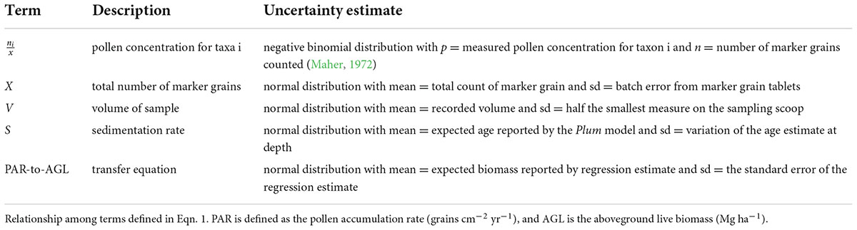
Table 1. Uncertainty estimates for the constituent metrics used to calculate tree biomass from pollen accumulation rates.
Sedimentation rate (S) depends on the precision of the age model and its error reflects the uncertainty in the model prediction. Recent advances in 210Pb age modeling using Bayesian-based software Plum provide estimates of uncertainty in ages (Aquino-López et al., 2018) compared to older approaches such as the constant rate of supply model that assume normal distributions for errors of the estimated ages (Appleby and Oldfield, 1978). In the context of PAR to biomass modeling, Plum software provides estimates of error continuously down core. We approximated uncertainty for specific ages at known depths by estimating the standard deviation from the 95% credible intervals reported by Plum (version 0.2.2 using default priors) in R (R Core Team, 2020; Table 1). Plots of all seven age-depth models can be found in Knight et al. (2021) Supplementary Material.
Pollen accumulation rates -biomass transfer function: Sources of uncertainty and recommended steps to apply the function
This function relies on estimating two key metrics: (1) the assemblage-level RSAP and (2) the modern biomass around lake sites. It is important to quantify the spatial extent represented by the pollen assemblage because the calibration of pollen-vegetation relationships is only effective when the scale of the vegetation sampling exceeds or is close to the scale of the RSAP (Bunting et al., 2004). An RSAP is unique to a given set of lakes and must be determined. However current practice (e.g., Seppä et al., 2009) is to rely on qualitative determinations of the pollen shed (e.g., “calibration zones”). Without an RSAP estimate, it is unknown whether the “calibration zones” of vegetation survey data from previous research were sufficiently extensive to create the PAR to biomass model.
Hence, we used the Extended R-Value method – we applied this using PolERV from the software suite HUMPOL (Bunting and Middleton, 2005) – to estimate pollen sheds (Knight et al., 2021). To evaluate the impact of model selection, we calculated both assemblage-level (aRSAP, 650 m) and taxa-specific (tRSAP) relevant source area pollen. Specifically, we compared results based on our chosen aRSAP to the four major tRSAPs on our landscape. The aRSAP and tRSAPs gave consistent interpretations of the source area of pollen and thus provided a means to cross-check an important model selection decision (Knight et al., 2021). The RSAP value has likely changed over time at these sites but estimating this change is difficult. Our RSAP estimate is a remaining source of uncertainty. However, assemblage-level RSAPs of small lakes may be relatively robust (Hellman et al., 2009).
Accurate estimation of biomass around lake sites is key to successfully calibrating transfer functions. Satellite-informed biomass estimates without ground truthing, or an absence of biomass measurements, are unsatisfactory for PAR-biomass calibration. For example, Seppä et al. (2009) used a remotely sensed product with a ± 44% error for aboveground live biomass. In Matthias and Giesecke (2014), biomass information was derived from yield tables linking tree age and tree standing volume. Neither paper provides sufficient detail to fully evaluate the measurement of biomass surrounding the lakes. Best practices would indicate that conducting detailed field surveys of vegetation surrounding the lake sites enhances the accuracy of biomass estimates conducting detailed field surveys of vegetation surrounding lake sites. For example, we used cruising prisms to determine basal area of dominant pollen-producing taxa within 750 m from the lake’s shore in eight directions (N,S,E,W,NE,SE,NW, and SW) at 50 m intervals (Knight et al., 2021). Note that vegetation survey method can profoundly affect model parameter estimates (Bunting and Hjelle, 2010) and recommendations for effective surveying methods for calibration with percentage vegetation cover are detailed in Bunting et al. (2013).
The last step in building the transfer function is the development of the PAR-to-biomass regression for each taxon. As described in Knight et al. (2021), we used an information theoretic approach to select the best model form. We retained standard errors of the estimate (SEE) to quantify uncertainty in the model predictions (Table 1).
Propagating errors
We calculated the uncertainty in our estimates by propagating the errors associated with the constituent terms (Table 1). Specifically, we used a Monte Carlo approach (Yanai et al., 2010; Harmon et al., 2015) to generate realizations of each term based on a random sample from a defined distribution (Table 1). We conducted the analysis in two parts.
First, we calculated the PAR terms (mean and standard error) for each lake at each date for every taxon combination. We conducted 1,000 simulations drawing samples with replacement for each constituent metric (Eqn. 1) and then calculated PAR. Prior to summarizing the PAR terms, we removed values beyond the 95% confidence intervals (n = 950 simulations retained). This trimming was necessary because random samples of the age model sometimes resulted in negative sedimentation rates, a physically unrealistic result. So as not to skew the error term, we trimmed both low and high values from the realizations.
In the second step, we used the PAR terms and the errors in the biomass transfer function to generate 1,000 realizations of aboveground live tree biomass for each lake at each date for every taxon combination. When these random realizations resulted in negative biomass estimates, a result restricted to instances of low pollen abundance, we set the biomass estimate to 0. For each realization, we summed tree biomass by lake and date and reported results (Figure 1) as the mean and standard error from these 1,000 realizations.
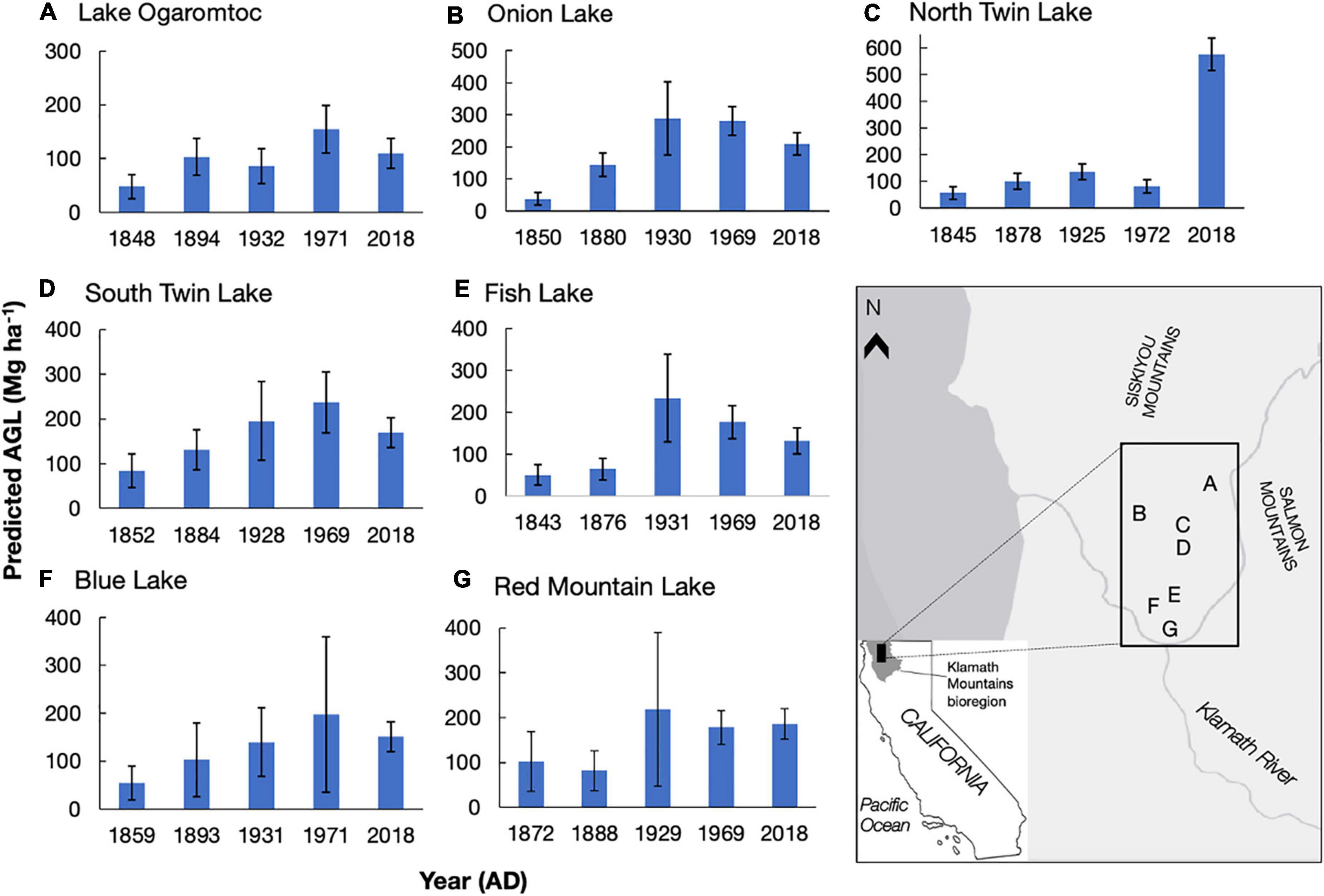
Figure 1. Predicted aboveground live tree biomass (AGL, Mg ha–1) for seven lake sites (A–G) at five time periods in the Klamath bioregion, California. AGL means and standard errors (calculated from uncertainty analysis) reported. Letters A-G correspond to the lake and its location on the map. Ages (year AD) were modeled from 210Pb dating presented in Knight et al. (2021) and reflect the mean age for that sampled cm. Biomass estimates reflect an area of ∼650 m around each lake site. Copyright © 2022 Esri and its licensors. All rights reserved.
Validating results
In QGIS (QGIS Development Team, 2020), the seven lake boundaries were plotted with spatial records of management events. Management events were compiled from the U.S. Forest Service Forest Activity Tracking System (FACTS, USDA Forest Service Forest Activity Tracking System, 2020) and an internal U.S. Forest Service dataset for the Six Rivers National Forest (USDA Forest Service, 2001). Definitions of the four silviculture treatments discussed below are as follows and taken from the USDA Forest Service (2019): patch clear cut (“a type of stand clear cutting where patches or strips are clear cut within an individual stand boundary in two or more entries to produce an even-aged stand”), even-aged cut (“the range of tree ages is usually less than 20 percent of the rotation after harvest of all patches”), sanitation cut (“a cutting to remove damaged trees”), and fuel break cut (“vegetative treatment to change fuel characteristics in such a way that expected fire behavior would be reduced”). A 650-m buffer was constructed around each lake, following the size of the sites’ assemblage-level RSAP (Knight et al., 2021). Using the “extract by location” tool in QGIS, all management events that fell within the buffers were extracted and were interpreted as relevant to the reconstructed biomass record.
Results
Results from seven lake sites
We detail trends in reconstructed tree biomass for five dates between ∼1850 AD and 2018 AD from seven lakes (Figure 1). In general, we found low mean biomass values (mean = 62 Mg ha–1) in the colonial era – a period starting in c. 1850 AD when colonization began in the Klamath region of California – and large increases in reconstructed biomass over time at all sites. Peak biomass varied at each site from early 20th century to early 21st century. While the overall trend in increased biomass following Euro-American colonization is due to effective landscape-level fire suppression starting in 1905 (Taylor and Skinner, 2003; Knight et al., 2020; Knight et al., 2022), variation in the timing of peak biomass depends on site-specific management histories.
The impact of these histories on biomass trends could sometimes be linked to timber harvests documented in the U.S. Forest Service FACTS database (USDA Forest Service Forest Activity Tracking System, 2020, also Conners, 1998). Twentieth century forest management events that occurred within the RSAP boundary and removed mature trees (e.g., clear cuts) were sometimes consistent with observed changes in biomass values across lake sites. For example, North Twin and South Twin lakes, which are situated within 100 m of each other and have partially overlapping RSAPs, are reconstructed as seeing increasing biomass between ∼1850 and ∼1930 (Figure 1). Two patch clear cuts adjacent to both lakes removed a total of 16.6 ha in 1971 (USDA Forest Service, 2001). At South Twin Lake, reconstructed biomass is 237 ± 68 Mg ha–1 (mean ± se) in 1969, before the clear cuts, whereas reconstructed biomass at North Twin Lake is 82 ± 26 Mg ha–1 in 1972, likely reflecting the loss of biomass from the clear cuts. Although changes in mean biomass may reflect silvicultural treatments within the RSAP, overlapping error bars preclude a definite link between the biomass trends and management events (e.g., the change in biomass from 1969 to 2018 at Onion Lake).
High biomass values (> 200 Mg ha–1) reflect the potential productivity of this fertile area. Although the highest biomass reconstructions were sometimes found in 2018 for our lakes, Lake Ogaromtoc did not follow this trend. At Lake Ogaromtoc, reconstructed biomass was relatively low throughout the record, with a peak of 155 ± 44 Mg ha–1 in 1971. While this result may be due to pollen shed specific characteristics such as the ridge that creates a scree slope on one side of the lake, the creation of four patch clear cuts and one fuel break between 1972 and 2008 covering about 40% of the pollen shed may have kept biomass relatively low (USDA Forest Service, 2001).
Results from error analysis
Uncertainty in the age model dominated the PAR error term (Table 2 and Supplementary Table 1). The coefficient of variation (cov) for the sedimentation rate was often one to two orders of magnitude greater than variation in the pollen concentration. As expected, error greatly increased for the older age estimates produced by the Plum model (i.e., deeper in the core). For example, the oldest modeled mean age at Fish Lake was 1843 AD with a range of 1821 to 1870 AD. By the mid-1900s, the sedimentation error term was equivalent in magnitude to the uncertainty in pollen concentrations.
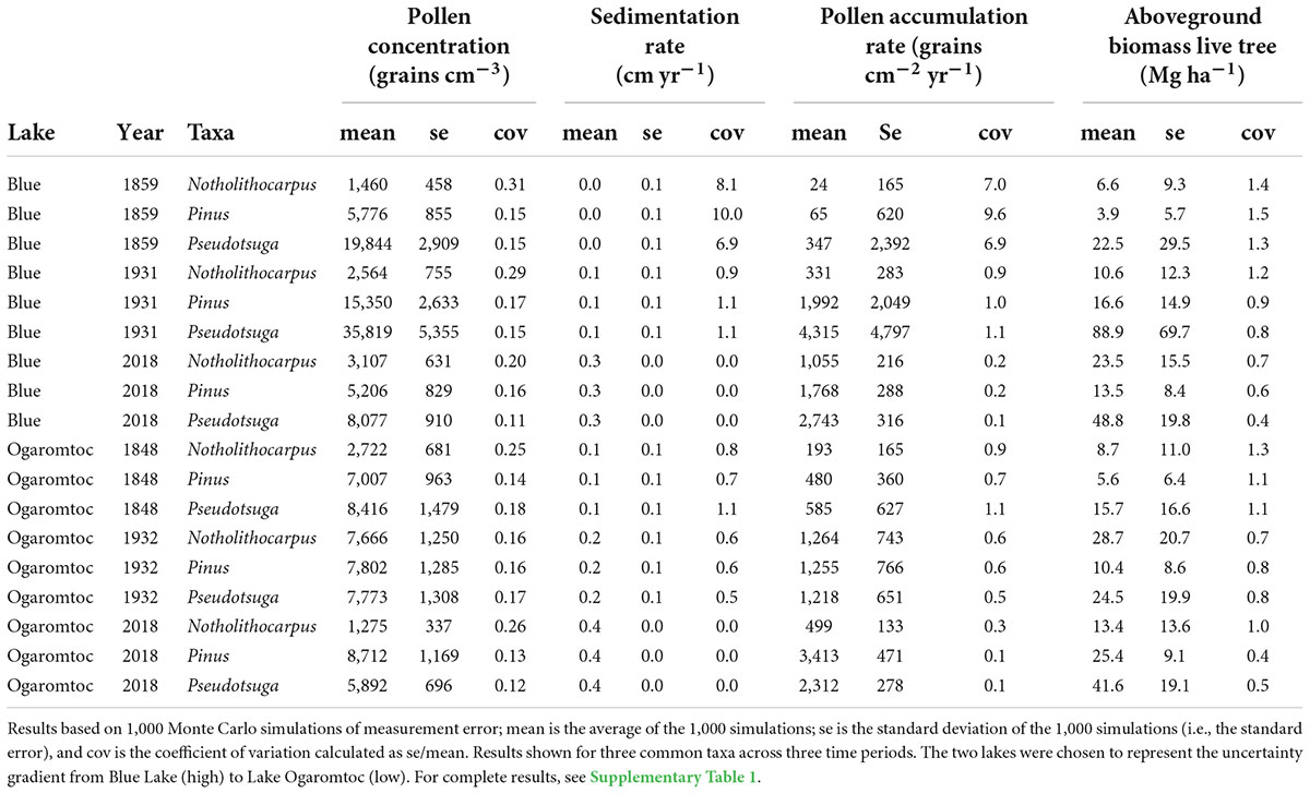
Table 2. Examples of the uncertainty associated with each step in the reconstruction of aboveground live tree biomass from pollen accumulation rates for seven lakes in the Klamath bioregion of California.
While the age-trend in PAR uncertainty affected estimates of aboveground live tree biomass (AGL), absolute error rates were reduced (Table 2). This reduction in error was due to the replacement of negative biomass predictions with zeros. This biological correction removed extreme values and thereby lowered overall estimates of uncertainty. Uncertainty in lake-by- date estimates of biomass (Figure 1) was further reduced summing across taxa. As a result, while there are certainly instances of large errors (e.g., cov = 0.82 for Blue Lake in 1971), they never exceed 1 (Figure 1).
Discussion
Uncertainty analysis identifies where error matters most
Accounting for the error in PAR estimates more than doubled the estimate of uncertainty in the reconstructions of aboveground live tree biomass. The coefficient of variation (cov) reported for contemporary to colonial-era biomass at Lake Ogaromtoc and Fish Lake ranged from 0.16 to 0.20 when only accounting for error in the PAR-to-biomass transfer function (Knight et al., 2022). Including uncertainty in PAR increased the range of observed cov from 0.22 to 0.48 (Figure 1). While this fuller account of uncertainty did not obscure the patterns observed with the transition from Indigenous to Euro-American stewardship, it does provide a more realistic estimate of the magnitude of change in forest biomass that can be reliably detected.
Our earlier work emphasized the importance of correctly modeling the RSAP and the PAR-to-biomass transfer function. In both cases, we applied robust methods to select the best supported model and thereby limited the potential to introduce errors related to model selection (sensu Harmon et al., 2015). Our expanded investigation of uncertainty highlighted the sensitivity of PAR estimates to the age model. This result underscores the need for improved statistical approaches to age modeling (Aquino-López et al., 2018). Future directions could include research to improve age-depth modeling techniques and standardization.
We deployed a combination of measurements (e.g., pollen concentration, forest biomass), models (e.g., age and pollen shed), and Monte Carlo simulations to account for uncertainty in our biomass proxy in a formal, coherent fashion. This empirical approach is particularly appropriate when the questions demand temporally and spatially fine-scale information (e.g., decadal trends for specific lakes). For more coarse-scale, regional inferences, Dawson et al. (2016) describe a bioproxy with full error accounting based on a Bayesian hierarchical spatial model which can be used when a large number of pollen records are available. Regardless of the specific approach, documenting the uncertainty in pollen vegetation models should be standard practice in paleoecology.
The usefulness of reconstructed biomass records
Reconstructed biomass records are particularly valuable where they can aid restoration plans and inform policy. For example, the state of California has crafted restoration and conservation strategies to ensure its vast forest ecosystems remain net sinks of carbon (Forest Climate Action Team, 2018). But these conservation goals may be unrealistic given recent research. For example, a landscape-wide historical reconstruction in the Sierra Nevada suggests that the pre-colonial forest supported low biomass (∼34 Mg/ha) (Bernal et al., 2022). Our results for the Klamath region also document low colonial-era biomass estimates (average 62 Mg/ha) consistent with Bernal et al. (2022). These historical reconstructions from California highlight the tension between realistic restoration goals and the State’s carbon policy (Forest Climate Action Team, 2018). The current high biomass and hence carbon storage is unlikely to be sustainable under climate change or compatible with acceptable management of fire risk (Bernal et al., 2022). The application of PAR-biomass transfer functions may shed light in other ecosystems where natural climate solutions are sought but there are mismatches in ecology and policy.
Author’s note
Any use of trade, firm, or product names is for descriptive purposes only and does not imply endorsement by the U.S. Government.
Data availability statement
Pollen data and age-depth model data from the seven lakes are publicly available online at https://doi.org/10.5066/P9HX7X5B (Knight, 2022).
Author contributions
CK, JB, DW, and JW contributed to conception and design of the study. CK and JW collected the data. CK organized the database and wrote the first draft of the manuscript. MC performed the laboratory analyses. JB performed the statistical analysis. CK, JB, and MB wrote the sections of the manuscript. All authors contributed to manuscript revision, read, and approved the submitted version.
Funding
Funding was provided by a grant from the California Department of Forestry and Fire Protection (18-CCI-FH-0007-SHU). This research was also supported by the U.S. Geological Survey Climate and Land Use Research and Development program, U.S. Forest Service (USFS) McIntire Stennis (Project 1020791), and the California Agricultural Research Station (CA-B-ECO-0144-MS).
Conflict of interest
The authors declare that the research was conducted in the absence of any commercial or financial relationships that could be construed as a potential conflict of interest.
Publisher’s note
All claims expressed in this article are solely those of the authors and do not necessarily represent those of their affiliated organizations, or those of the publisher, the editors and the reviewers. Any product that may be evaluated in this article, or claim that may be made by its manufacturer, is not guaranteed or endorsed by the publisher.
Supplementary material
The Supplementary Material for this article can be found online at: https://www.frontiersin.org/articles/10.3389/fevo.2022.956143/full#supplementary-material
References
Appleby, P., and Oldfield, F. (1978). The calculation of lead-210 dates assuming a constant rate of supply of unsupported 210Pb to the sediment. Catena 5, 1–8. doi: 10.1016/S0341-8162(78)80002-2
Aquino-López, M. A., Blaauw, M., Christen, J. A., and Sanderson, N. K. (2018). Bayesian analysis of 210-Pb dating. J. Agric. Biol. Environ. Stud. 23:317. doi: 10.1016/j.dib.2022.108444
Bernal, A. A., Stephens, S. L., Collins, B. M., and Battles, J. J. (2022). Biomass stocks in California’s fire-prone forests: Mismatch in ecology and policy. Environ. Res. Lett. 17:044047. doi: 10.1088/1748-9326/ac576a
Birks, H. J. B. (1995). “Quantitative palaeoenvironmental reconstructions,” in Statistical Modeling of Quaternary Science Data. Technical Guide 5, eds D. Maddy and J. S. Brew (Cambridge, MA: Quaternary Research Association), 116–254.
Bunting, M. J., Farrell, M., Broström, A., Hjelle, K. L., Mazier, F., Middleton, R., et al. (2013). Palynological perspectives on vegetation survey: A critical step for model-based reconstruction of Quaternary land cover. Quat. Sci. Rev. 82, 41–55. doi: 10.1016/j.quascirev.2013.10.006
Bunting, M. J., Gaillard, M.-J., Sugita, S., Middleton, R., and Broström, A. (2004). Vegetation structure and pollen source area. Holocene 14, 651–660. doi: 10.1191/0959683604hl744rp
Bunting, M. J., and Hjelle, K. L. (2010). Effect of vegetation data collection strategies on estimates of relevant source area of pollen (RSAP) and relative pollen productivity estimates (relative PPE) for non-arboreal taxa. Veg. Hist. Archaeobot. 19, 365–374. doi: 10.1007/s00334-010-0246-2
Bunting, M. J., and Middleton, R. (2005). Modeling pollen dispersal and deposition using HUMPOL software: Simulating wind roses and irregular lakes. Rev. Palaeobot. Palynol. 134, 185–196. doi: 10.1016/j.revpalbo.2004.12.009
Cain, S. A. (1939). Pollen analysis as a paleo-ecological research method. Bot. Rev. 5, 627–654. doi: 10.1007/BF02871650
Conners, P. A. (1998). A history of the Six Rivers National Forest: Commemorating the First 50 Years. Washington, DC: USDA Forest Service.
Davies, A. L., and Bunting, M. J. (2010). Applications of palaeoecology in conservation. Open Ecol. J. 3, 54–67. doi: 10.2174/1874213001003020054
Davis, M. B., and Deevey, E. S. (1964). Pollen accumulation rates: Estimates from late-glacial sediment rogers Lake. Science 145, 1293–1295. doi: 10.1126/science.145.3638.1293
Dawson, A., Paciorek, C. J., McLachlan, J. S., Goring, S., Williams, J. W., and Jackson, S. T. (2016). Quantifying pollen-vegetation relationships to reconstruct ancient forests using 19th-century forest composition and pollen data. Quat. Sci. Rev. 137, 156–175. doi: 10.1016/j.quascirev.2016.01.012
Doher, L. I. (1980). Palynomorph preparation procedures currently used in the paleontology and stratigraphy laboratories, U.S. geological survey. Circular 830, 1–28. doi: 10.3133/cir830
Forest Climate Action Team (2018). California forest carbon plan: Managing our forest landscapes in a changing climate p 186. Available online at: https://resources.ca.gov/CNRALegacyFiles/wpcontent/uploads/2018/05/California-Forest-Carbon-Plan-Final-Draft-for-Public-Release-May-2018.pdf
Gaillard, M.-J., Sugita, S., Mazier, F., Trondman, A. K., Broström, A., Hickler, T., et al. (2010). Holocene land-cover reconstructions for studies on land cover-climate feedbacks. Clim. Past 6, 483–499. doi: 10.5194/cp-6-483-2010
Giesecke, T., and Fontana, S. L. (2008). Revisiting pollen accumulation rates from Swedish lake sediments. Holocene 18, 293–305. doi: 10.1177/0959683607086767
Halbritter, H., Ulrich, S., Grímsson, F., Weber, M., Zetter, R., Hesse, M., et al. (2018). Illustrated Pollen Terminology. Berlin: Springer International Publishing. doi: 10.1007/978-3-319-71365-6
Harmon, M. E., Fasth, B., Halpern, C. B., and Lutz, J. A. (2015). Uncertainty analysis: An evaluation metric for synthesis science. Ecosphere 6, 1–12. doi: 10.1890/ES14-00235.1
Hellman, S., Bunting, M. J., and Gaillard, M.-J. (2009). Relevant source area of pollen in patchy cultural landscapes and signals of anthropogenic landscape disturbance in the pollen record: A simulation approach. Rev. Palaeobot. Palynol. 153, 245–258. doi: 10.1016/j.revpalbo.2008.08.006
Hickman, J. C. (1993). The Jepson Manual: Higher Plants of California. Berkeley, CA: University of California Press.
Hicks, S., and Hyvarinen, H. (1999). Pollen influx values measured in different sedimentary environments and their palaeoecological implications. Grana 38, 228–242. doi: 10.1080/001731300750044618
Jackson, S. T., and Overpeck, J. T. (2000). Responses of plant populations and communities to environmental changes of the late quaternary. Paleobiology 26, 194–220. doi: 10.1017/S0094837300026932
Juggins, S., and Birks, H. J. B. (2012). “Quantitative environmental reconstructions from biological data,” in Tracking Environmental Change Using Lake Sediments. Developments in Paleoenvironmental Research, Vol. 5, eds H. Birks, A. Lotter, S. Juggins, and J. Smol (Dordrecht: Springer). doi: 10.1007/978-94-007-2745-8_14
Knight, C. A. (2022). Pollen data from seven lakes in the Klamath Mountains, California: A case study for paleoecological reconstruction. U.S. Geological Survey data Release. doi: 10.5066/P9HX7X5B
Knight, C. A., Anderson, L., Bunting, M. J., Champagne, M., Clayburn, R., Crawford, J., et al. (2022). Land management explains major trends in forest structure and composition over the last millennium in California’s Klamath Mountains. Proc. Natl. Acad. Sci. 119:e2116264119. doi: 10.1073/pnas.2116264119
Knight, C. A., Baskaran, M., Bunting, M. J., Champagne, M., Potts, M. D., Wahl, D., et al. (2021). Linking modern pollen accumulation rates to biomass: Quantitative vegetation reconstruction in the western Klamath Mountains. Holocene 31, 814–829. doi: 10.1177/0959683620988038
Knight, C. A., Cogbill, C. V., Potts, M. D., Wanket, J. A., and Battles, J. J. (2020). Settlement-era forest structure and composition in the Klamath Mountains: Reconstructing a historical baseline. Ecosphere 11:e03250. doi: 10.1002/ecs2.3250
Köhl, M., Lasco, R., Cifuentes, M., Jonsson, Ö, Korhonen, K. T., Mundhenk, P., et al. (2015). Changes in forest production, biomass and carbon: Results from the 2015 UN FAO global forest resource assessment. For. Ecol. Manag. 352, 21–34. doi: 10.1016/j.foreco.2015.05.036
Maher, L. J. Jr. (1972). Nomograms for computing 0.95 confidence limits of pollen data. Rev. Palaeobot. Palynol. 13, 85–93. doi: 10.1016/0034-6667(72)90038-3
Maher, L. J. Jr. (1981). Statistics for microfossil concentration measurements employing samples spiked with marker grains. Rev. Palaeobot. Palynol. 32, 153–191. doi: 10.1016/0034-6667(81)90002-6
Matthias, I., and Giesecke, T. (2014). Insights into pollen source area, transport and deposition from modern pollen accumulation rates in lake sediments. Quat. Sci. Rev. 87, 12–23. doi: 10.1016/j.quascirev.2013.12.015
Morris, J. L., DeRose, J. R., and Brunelle, A. R. (2015). Long-term landscape changes in a subalpine spruce-fir forest in central Utah, USA. For. Ecosyst. 2, 1–12. doi: 10.1186/s40663-015-0057-0
Parsons, R. W., Gordon, A. D. I, and Prentice, C. (1983). Statistical uncertainty in forest composition estimates obtained from fossil pollen spectra via the R-value model. Rev. Palaeobot. Palynol. 40, 177–189. doi: 10.1016/0034-6667(83)90035-0
Prentice, I. C., and Parsons, R. W. (1983). Maximum likelihood linear calibration of pollen spectra in terms of forest composition. Biometrics 39, 1051–1057. doi: 10.2307/2531338
QGIS Development Team (2020). QGIS Geographic Information System. Beaverton, OR: Open-source geospatial foundation.
R Core Team (2020). R: A Language and Environment for Statistical Computing R Foundation for Statistical Computing. Vienna: R Core Team.
Sawyer, J. O., and Thornburg, D. A. (1977). “Montane and subalpine vegetation of the Klamath Mountains,” in Terrestrial Vegetation of California, eds M. G. Barbour and J. Major (Berkeley, CA: California Native Plant Society), 699–732. doi: 10.1007/s00484-017-1449-3
Seppä, H., Alenius, T., Muukkonen, P., Giesecke, T., Miller, P. A., and Ojala, A. E. K. (2009). Calibrated pollen accumulation rates as a basis for quantitative tree biomass reconstructions. Holocene 19, 209–220. doi: 10.1177/0959683608100565
Seppä, H., and Hicks, S. (2006). Integration of modern and past pollen accumulation rate (PAR) records across the arctic tree-line: A method for more precise vegetation reconstructions. Quat. Sci. Rev. 25, 1501–1516. doi: 10.1016/j.quascirev.2005.12.002
Sugita, S. (1993). A model of pollen source area for an entire lake surface. Quat. Res. 39, 239–244. doi: 10.1006/qres.1993.1027
Taylor, A. H., and Skinner, C. N. (2003). Spatial patterns and controls on historical fire regimes and forest structure in the Klamath Mountains. Ecol. Appl. 13, 704–719. doi: 10.1890/1051-0761(2003)013[0704:SPACOH]2.0.CO;2
USDA Forest Service (2001). Six rivers national forest: Vegetation plant associations, sub-series and seral stages of the six rivers national forest: In-house spatial dataset on file. Eureka, CA: Six Rivers National Forest.
USDA Forest Service (2019). FACTS User Guide Appendix B: Activity Codes. New York, NY: United Nations Department.
Whittaker, R.H. (1960). Vegetation of the Siskiyou mountains, Oregon and California. Ecol. Monogr. 30, 279–338. doi: 10.1002/ecy.3764
Keywords: biomass proxy, forest dynamics, pollen-vegetation modeling, pollen, uncertainty analysis
Citation: Knight CA, Battles JJ, Bunting MJ, Champagne M, Wanket JA and Wahl DB (2022) Methods for robust estimates of tree biomass from pollen accumulation rates: Quantifying paleoecological reconstruction uncertainty. Front. Ecol. Evol. 10:956143. doi: 10.3389/fevo.2022.956143
Received: 29 May 2022; Accepted: 18 July 2022;
Published: 25 August 2022.
Edited by:
Anna Maria Mercuri, University of Modena and Reggio Emilia, ItalyCopyright © 2022 Knight, Battles, Bunting, Champagne, Wanket and Wahl. This is an open-access article distributed under the terms of the Creative Commons Attribution License (CC BY). The use, distribution or reproduction in other forums is permitted, provided the original author(s) and the copyright owner(s) are credited and that the original publication in this journal is cited, in accordance with accepted academic practice. No use, distribution or reproduction is permitted which does not comply with these terms.
*Correspondence: Clarke A. Knight, Y2tuaWdodEB1c2dzLmdvdg==