 Boris Espinasse1*
 Anthony Sturbois2,3
 Sünnje L. Basedow1
 Pierre Hélaouët4
 David G. Johns4
 Jason Newton5
 Clive N. Trueman6
- 1Department of Arctic and Marine Biology, UiT The Arctic University of Norway, Tromsø, Norway
- 2Laboratoire des Sciences de l’Environnement Marin (LEMAR), UMR 6539 CNRS/UBO/IRD/IFREMER, Plouzané, France
- 3Vivarmor Nature, Ploufragan, France
- 4The Marine Biological Association, Plymouth, United Kingdom
- 5National Environmental Isotope Facility (NEIF), Scottish Universities Environmental Research Centre (SUERC), East Kilbride, United Kingdom
- 6School of Ocean and Earth Science, University of Southampton, Southampton, United Kingdom
The limited amount of ecological data covering offshore parts of the ocean impedes our ability to understand and anticipate the impact of anthropogenic stressors on pelagic marine ecosystems. Isoscapes, i.e., spatial models of the distribution of stable isotope ratios, have been employed in the recent years to investigate spatio-temporal patterns in biogeochemical process and ecological responses. Development of isoscapes on the scale of ocean basins is hampered by access to suitable reference samples. Here we draw on archived material from long-running plankton survey initiatives, to build temporally explicit isoscape models for the North Atlantic Ocean (> 40°N). A total of 570 zooplankton samples were retrieved from Continuous Plankton Recorder archives and analysed for δ13C and δ15N values. Bayesian generalised additive models were developed to (1) model the relations between isotopic values and a set of predictors and (2) predict isotopic values for the whole of the study area. We produced yearly and seasonal isoscape models for the period 1998–2020. These are the first observation-based time-resolved C and N isoscapes developed at the scale of the North Atlantic Ocean. Drawing on the Stable Isotope Trajectory Analysis framework, we identify five isotopically distinct regions. We discuss the hydro-biogeochemical processes that likely explain theses modes, the differences in temporal dynamics (stability and cycles) and compare our results with previous bioregionalization efforts. Finally, we lay down the basis for using the isoscapes as a tool to define predator distributions and their interactions with the trophic environment. The isoscapes developed in this study have the potential to update our knowledge of marine predator ecology and therefore our capacity to improve their conservation in the future.
Introduction
Oceans have been under continuous and increasing anthropogenic pressure over the last two centuries (Halpern et al., 2019). The diversity of the stressors, and their combined and interactive effects complicate the study of their impacts on marine ecosystems (Bundy et al., 2021; Heneghan et al., 2021). In addition, several gaps in our knowledge still hamper our ability to characterise how stressors affect different components of the ecosystem and to anticipate their evolution in the future. In particular, there is a need to distinguish between internal dynamic, natural variability intrinsic to the ecosystem, and stressor-induced variability that might result in irreversible shifts in ecosystem structure and functioning (Scheffer et al., 2001; Henson et al., 2017). Fundamental knowledge on spatial distribution of species and populations and their interactions is also commonly missing, particularly in remote, inaccessible regions such as ocean basins. To overcome these challenges, observational-based multidisciplinary datasets with resolutions matching spatio-temporal dynamics of ecological processes occurring in the oceans are needed. While monitoring programs are common in coastal areas, the offshore part of the oceans remains poorly monitored due to very large spatial scales, and the associated expense and logistical challenges of sampling the animals and their environment (Richardson and Poloczanska, 2008).
New approaches are being developed to fill observational gaps. Among them, natural biogeochemical tracers present the advantage of recording various parameters on in situ conditions experienced by animals, suitable for later retrospective analysis (McMahon et al., 2013a). Spatio-temporal variations of natural abundance stable isotope (SI) ratios of carbon and nitrogen (expressed as δ13C and δ15N values) have been widely used during the last decades to infer aspects of hydrological conditions (Kline, 1999), nutrient sources and limitations (Rau et al., 1991; Hobson et al., 1995), animal movement or trophic level (Jennings and Warr, 2003; Cherel and Hobson, 2007). Spatial modelling (mapping) of SI ratios at the base of the food web (with spatial models commonly termed “isoscapes”; West et al., 2010), allows consideration of underlying biogeochemical drivers responsible for producing spatial pattern in isotope ratios as well as providing a reference to interpret stable isotope compositions measured in tissues of mobile consumers (McMahon et al., 2013b; Trueman and St John Glew, 2019). Isoscapes can be produced using mechanistic (theoretical) or observation-based (statistical) approaches (Bowen, 2010). Mechanistic models have the advantage of producing isoscapes at global scale and potentially allow projection forward and backward in time (Tagliabue and Bopp, 2008; Schmittner and Somes, 2016), but their spatial resolution is limited by the data used to feed the model, the complexity of model structures required to represent biogeochemical reality and our incomplete understanding of the isotopic expression of biogeochemical processes (e.g., nitrate map). Observation-based isoscapes can be developed either by using simple interpolation methods (e.g., Schell et al., 1998) or can be modelled based on predictors to reinforce prediction power where observations are not available (St John Glew et al., 2019). Such isoscapes have already been produced in different places, including the North Pacific Ocean (Espinasse et al., 2020a), the North Sea (Mackenzie et al., 2014), the Arctic Ocean (Buchanan et al., 2021), and the Southern Ocean (St John Glew et al., 2021).
The North Atlantic Ocean is one of the most studied marine areas in the world, with some of the oldest monitoring programs still in activity (Hays et al., 2005). Major ecological concepts were established there, including the match-mismatch hypothesis (Cushing, 1990) with deep consequences on our understanding of cascading effects of climate change in marine ecosystems (Beaugrand et al., 2003; Chivers et al., 2017). Despite the intense study and detailed observation, only one interpolation model of SI variations in carbon and nitrogen across the North Atlantic is currently available (McMahon et al., 2013b), based on relatively sparsely distributed reference data. In this study, we use a long-term monitoring program to access samples of Calanus, a large copepod collected along transects across the North Atlantic Ocean. These copepods play a major role both by transferring carbon toward higher trophic levels, but also in the biological pump by contributing to the sequestration of carbon in the ocean bottom (Brun et al., 2019). We modelled yearly and seasonal isoscapes based on Calanus isotopic composition and environmental variables for 1998–2020. The objectives were (1) to identify ecoregions with similar isotopic regime, (2) to describe the temporal dynamic (variability and trend) in carbon and nitrogen isoscapes, and (3) to lay the basis for future applications.
Materials and methods
Zooplankton sample collection
Zooplankton samples were retrieved from the archives of the Continuous Plankton Recorder (CPR) survey. The CPR survey consistent methodology started in 1958, and over a quarter of a million samples have been processed since then. Sample collection is made with an autonomous plankton sampler towed by ships of opportunity along their monthly commercial routes. The system does not need electrical power or human handling (other than putting the instrument in the water and retrieving it). It collects plankton in sub surface water (about 7–9 m depth) using a continuously moving band of filter silk. The silk is further divided into samples, each representing a ten nautical miles piece of transect (for a volume of about 3 m3 of filtered water).
The extent of the study area was roughly designed by the occurrence of CPR samples and therefore covers the northern part of the North Atlantic Ocean from 40°N to 72°N and from 60°W to 16°E (Figure 1). We specifically target large herbivorous copepods, aiming to produce an isotopic baseline as consistent as possible by limiting inter-sample differences in trophic level. Calanus finmarchicus and Calanus helgolandicus are two congeneric calanoid copepod species with a similar life cycle which includes lipid storage and seasonal diapause in deep water (Wilson et al., 2015). The core distribution area of the two species is separated by the North Atlantic current, which flows across the North Atlantic Ocean from SW to NE. A total of 570 samples (CV and adult stages) were selected to cover the whole study area with both species being selected, although C. finmarchicus was predominantly used (n = 511).
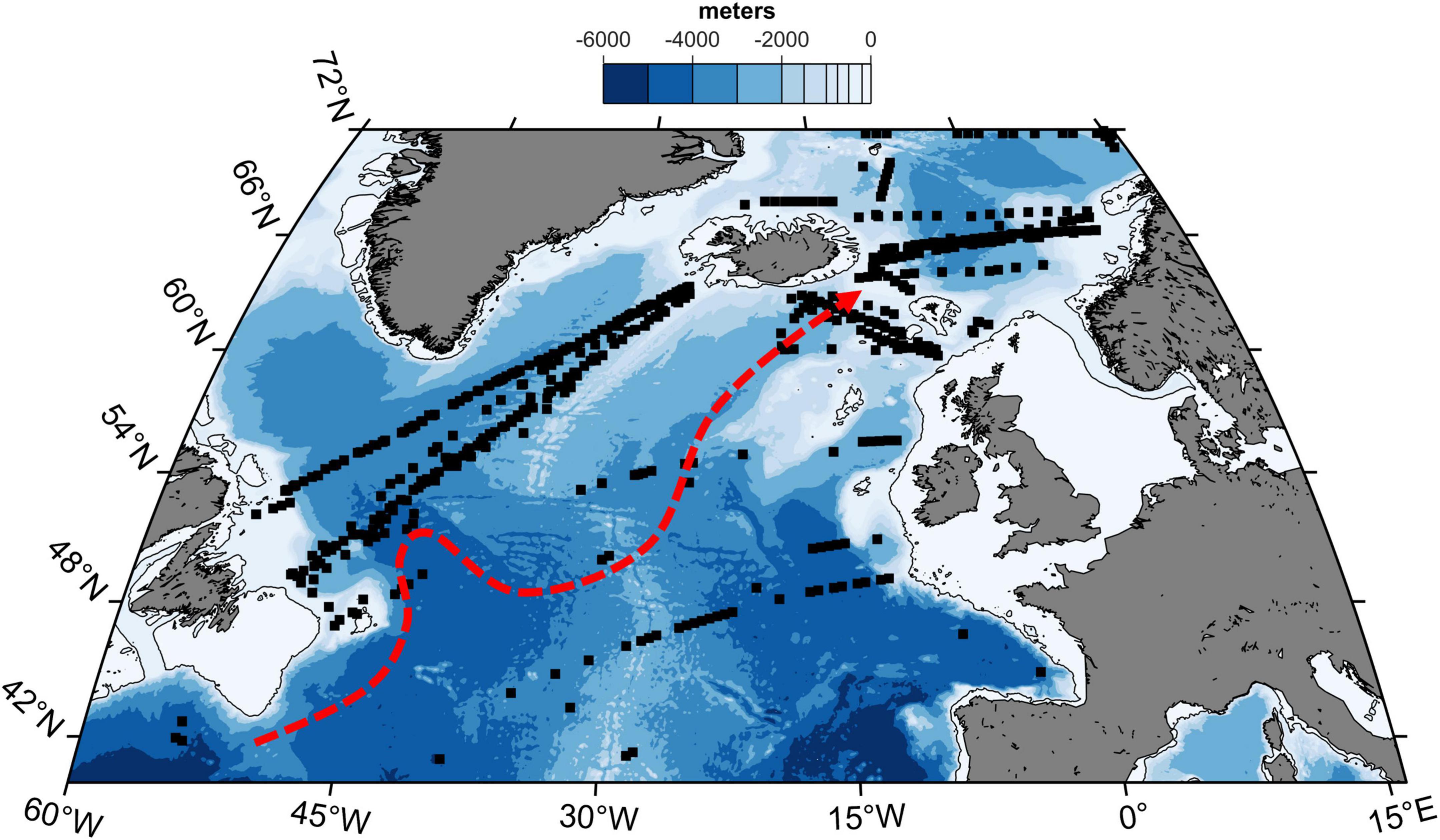
Figure 1. Location of zooplankton samples collected in the North Atlantic Ocean (> 40°N). The 200 m isobath is shown (thin black line). Dashed red line show approximate position of the main branch of the North Atlantic Current (from Drinkwater et al., 2020).
The samples were selected from the CPR list, including several thousands of entries. The rationale behind the sample selection consisted of: presence of C. finmarchicus or C. helgolandicus in numbers required for SI analysis; availability of ocean colour data (subject to cloud coverage); distance of 50 km from the 200 m isobath; to represent most ecoregions defined in Beaugrand et al. (2019). The samples were selected within a 10-year time window 2009–2018, which is wide enough to smooth interannual variability, but still allow to have a significant number of samples for each year.
The main mechanisms driving changes in isotopic values of lower trophic level are not necessarily the same in coastal environments and in open ocean. Freshwater runoff, sediment resuspension and terrestrial inputs are some of the drivers that can dramatically affect isotopic values of organisms onto the shelf. Physical processes in coastal area tend to be highly variable in time, and complexify the modelling of relationship between parameters and observed isotopic composition. In the frame of this study, we focused on the offshore part of the ocean and therefore did not include a 50 km width band from the 200 m isobath.
We aimed to produce yearly as well as seasonal isoscapes. Seasonal time windows ideally maximise temporal variation among seasons while minimising temporal variance within seasons. Time windows for the seasonal isoscapes were defined based on sample availability and the state of the system (dynamic vs. stable). Relatively few samples are available from November to February, removing this time period as an option. The width of the time window needs to be large enough to provide sufficient samples to resolve a spatial model (we aim for 100 samples per time window). Also, tissues from individuals with different growth and metabolic rates reflect integration across varying timeframes so it is better to select a time window during which the ecosystem is relatively temporally consistent in terms of productivity, so that the isotopic values are stabilised. Taking these aspects in consideration (see Supplementary Figure 1), three seasonal time windows were defined: winter, mid-February to end of March (n = 90); summer, June (n = 300); and fall, mid-September to mid-October (n = 180).
Isotopic analysis
Isotopic ratios are expressed in the following standard notation δX = Rsample/Rstandard – 1, where X is 13C or 15N and R is the 13C/12C or 15N/14N. The δ13C and δ15N values are expressed in parts per thousand (‰) relative to external standards of Vienna Pee Dee Belemnite and atmospheric nitrogen, respectively. All samples were dried, encapsulated in tin foil and sent for SI analysis at the Scottish Universities Environmental Research Centre (SUERC) as part of National Environmental Isotope Facility (NEIF). Samples were loaded into an Elementar (Hanau, Germany) Pyrocube elemental analyser, which converted carbon and nitrogen in the samples to CO2 and N2 gases. δ13C and δ15N of evolved gases were measured on a Thermo-Fisher-Scientific (Bremen, Germany) Delta XP Plus isotope ratio mass spectrometer. The system was calibrated using laboratory standards and then independently checked for accuracy using USGS 40 glutamic acid reference material (Qi et al., 2003; Coplen et al., 2006). Measurement precision was assessed by running replicates of laboratory standards and resulted in a SD consistently < 0.1‰ and 0.2‰ for δ13C and δ15N, respectively. A quality check was performed to discard samples having too low C or N mass, resulting in n = 506 for δ15N and n = 567 for δ13C.
The sampling procedure of the CPR survey includes instantaneous conservation of the samples with 4% buffered formalin (Batten et al., 2003). Effects of formalin preservation on copepod isotopic composition have been shown to be negligible on δ15N values and small on δ13C values (Hetherington et al., 2019), with most of the effects occurring within the first weeks (Bicknell et al., 2011). In order to facilitate the comparison with other studies, we applied correction factors specifically developed for copepods sampling within the CPR survey (+0.68 and –0.33 for δ13C and δ15N, respectively) (Bicknell et al., 2011).
Because Calanus store lipids and lipids are depleted in 13C relative to proteins and carbohydrates, it is common to correct δ13C values to remove effect of lipid content (Kiljunen et al., 2006; Post et al., 2007; Logan et al., 2008). High lipid content results in high carbon biomass and higher Carbon-to-Nitrogen (CN) ratios. Therefore, CN ratios are commonly used to establish correction model. However, CN ratios appeared to be very stable through samples (4.41 ± 0.43), close to expected values for chitinous copepod samples with little or no lipid content (El-Sabaawi et al., 2009; Espinasse et al., 2014). This might be due to the sampling procedure that tends to squeeze the copepods between the silks. We did not then correct δ13C values for lipids.
Carbon dioxide originating from fossil fuel burning is also depleted in 13C. With the increase of CO2 concentration in the atmosphere driven by anthropogenic activities, δ13C values follow a negative trend known as the Suess effect (Gruber et al., 1999). In the oceans, which capture a large part of CO2, δ13C values of autotroph organisms are impacted via two mechanisms. The Suess effect itself, which result in lowering δ13C values for aqueous CO2, and the increase in aqueous CO2 concentration, which allows phytoplankton to use more 12C, their preferential isotope. The combination of these two mechanisms results in an exponential decrease of δ13C values at the base of the food webs, with the effect getting stronger in recent years (Espinasse et al., 2018). We correct our data using 2015 as a reference year. The correction factors were provided by the R-package SuessR (Clark et al., 2021).
Environmental variables
A range of variables were considered to produce parameters used to explain zooplankton SI variability. The main constraint was to obtain a consistent dataset covering the whole study area with good spatial resolution, and being available for a time period matching at least 2009–2018 (SI data). Observational data were prioritised. Available variables were: chlorophyll-a concentration (chla), net primary production (NPP), sea surface temperature (SST), wind speed (wind), mixed layer depth (MLD), and distance to the shelf (dist). Data were provided in various resolutions before being projected onto a 0.25° grid. All datasets were retrieved from the European Union Copernicus Marine Environmental Monitoring Service (CMEMS).1 SST were extracted from the Operational Sea Surface Temperature and Ice Analysis (OSTIA) product, provided by the UK’s Met Office. OSTIA uses satellite data provided by the GHRSST project together with in situ observations to determine the sea surface temperature (Good et al., 2020). MLD was issued from the GLORYS12V1 product, which is a global ocean eddy-resolving reanalysis covering the satellite altimetry period 1993--2018. Wind data were provided by IFREMER, France. The product consists of L4 satellite-derived observations using scatterometer. Chla concentrations were collected from GlobColour.2 GlobColour delivers a merged product that uses all satellite data available at the processing time (Maritorena et al., 2010). All Chla data used in this study has been developed, validated, and distributed by ACRI-ST, France. NPP was computed using the Eppley Vertically Generalized Production Model (Eppley-VGPM) calculation. The Eppley-VGPM calculation was adapted from the VGPM approach (Behrenfeld and Falkowski, 1997), in which the polynomial description of light-saturated photosynthetic efficiencies as a function of SST is replaced with the exponential relationship described by Morel (1991) and based on the curvature of the temperature-dependent growth function described by Eppley (1972). The script for the calculation was acquired from Oregon State University.3 Chla and NPP products are dependent on atmospheric conditions, resulting in missing data for some areas due to persistent cloud coverage. The distance to the shelf (dist) was calculated as distance from the centre point of the grid cell to the 200 m isobath, based on ETOPO1 Global Relief Model. Each environmental covariate value was extracted at each sampling location.
Isotopic values of copepods sampled at a given time cannot systematically be explained by local, immediate environmental conditions (Rolff, 2000). Indeed, a change in environmental conditions might take a few days to be reflected into autotroph isotopic composition (driven by a wide range of factors including environmental conditions, phytoplankton composition, growth, and shape). As all heterotrophs, Calanus SI values are influenced by the isotopic baseline and the trophic structure linking the base of the food webs to the copepods. Therefore, isotopic composition of the autotrophs is not necessarily transferred directly into zooplankton. However, the presence of an intermediate trophic step between phytoplankton and herbivorous zooplankton, i.e., protozoan, was shown to not significantly affect zooplankton δ15N values (Gutiérrez-Rodríguez et al., 2014). Furthermore, once the new conditions stabilise, it is the tissue turnover rate of copepods that will define when the final isotopic values are reached. It is estimated to take about 1–2 weeks for copepods (Graeve et al., 2005; Tiselius and Fransson, 2016). During this time, the animals are transported around with water masses and might experience different conditions complexifying the picture. We tested a range of integration windows for the environmental variables and concluded that 2 months produce the best models for explaining observed SI data.
Model development
Model development and metrics production were conducted using the software environment R v.4.1.3 (R Core Team, 2022). All maps were produced using the m_map package (Pawlowicz, 2019) running under Matlab 2020a. To produce isoscapes, we used the following sequence: (1) obtaining geo-referenced SI dataset, (2) extracting environmental variables at sampling locations and times, (3) carrying preliminary dataset checks, (4) selecting the best models using a frequentist approach, (5) implementing spatial component using Bayesian framework, and (6) predicting SI values for the whole study area using the modelled relationship and continuously observed environmental variables as predictors. The first two steps were introduced above.
We followed the protocol detailed by Zuur et al. (2010) for data exploration. Covariates were checked for outliers, normal distribution, and collinearity. It implied to log transform or cap some of the parameters (see Supplementary Table 1 for details). The covariate NPP was removed in the process (variance-inflation factors, VIF > 5).
We developed several frequentist Generalized Additive models (GAMs) using the “mgcv” R-package (Wood et al., 2016; Wood, 2017). GAM are semi-parametric extensions of Generalized Linear Models, which allows the use of smoothers to fit covariates. The procedure for model selection includes trying several predictor combinations, defining the number of knots for the smoothers and comparing model efficiency (Akaike information criterion, AIC) (Akaike, 1974).
The Bayesian hierarchical spatial modelling framework, Integrated Nested Laplace Approximation (INLA) (Rue et al., 2009), was demonstrated to be a powerful spatial statistical package to produce isoscapes (St John Glew et al., 2019). Compared to the frequentist mixed modelling approach, the Bayesian framework enable uncertainty to be more easily interpretable, allow the inclusion of boundary effects and solve the spatial dependency term in an alternative and faster way. We used the guidelines in Lindgren and Rue (2015) to write and structure the code with the R-INLA package, and from Zuur et al. (2017) to adapt frequentist GAM smoothers to INLA. This allowed a better control on the number of knots which define the “wiggliness” of the smoothers (i.e., the amount of smoothing). In ecological studies, where datasets are often sparse and fragmented, it is recommended to apply greater amount of smoothing to dampen wiggliness as high-frequency variations in poorly constrained smooth terms can result in models which are too specific to the dataset and makes difficult to relate smoother shapes and ecological processes.
where Yi is the isotope value (δ13C, δ15N) at location i; b is the intercept, fn are smooth functions (thin plate regression splines in this case), and Xn are the covariates; Wi represents the smooth spatial effect, linking each observation with a spatial location. INLA uses the Stochastic Partial Differential Equations (SPDE) approach for the spatial effect (Lindgren et al., 2011). The SPDE approach enables the covariance matrix of the Gaussian field to be approximated as a Gaussian Markov Random Field using a Matérn covariance structure and Delaunay triangulation to create prediction locations in the form of a mesh (Supplementary Figure 2). The Matérn covariance function has two hyperparameters: the marginal standard deviation σ and κ (smoothness of the field, relates to the range r). As recommended by Fuglstad et al. (2019), we set priors for these two parameters such as P(r < 100 km) = 0.01 and P(σ > 2) = 0.01.
All the models were validated by checking the homogeneity of variance and the normal distribution of residuals and by investigating any pattern in the plot of residuals against predictors (Zuur, 2012). The best fit models were used to predict δ13C and δ15N values across the whole North Atlantic Ocean spatial domain using environmental variables as predictors. Response variables were estimated at all mesh vertices which were then linearly interpolated within each triangle into a finer regular grid (0.25°) via Bayesian kriging. Mean and variance predictions were obtained for each grid cell. To ensure that predicted values fell within a sensible range, environmental variable surfaces were assessed to check that all values used for predictions fell within the range of values observed at zooplankton sampling locations (± 10%). Outlier grid cells were blanked from maps. Isoscapes were produced over the time period for which environmental variables were available, i.e., 1998–2020.
Several approaches can be used to model seasonal isoscapes using GAM: (1) splitting the dataset and developing independent models for each season, (2) using the global dataset and including season as a fixed effect,or (3) using the global dataset to develop a universal model and making predictions with seasonally explicit sets of predictors. Our dataset did not allow for the first option as not enough data were available for each season, especially for winter. The two other options gave similar results when comparing observation and modelled values at sampling locations (using frequentist models without spatial component) (Supplementary Figure 3). The third option was favoured over the second one because it resulted in simpler model structure.
Trajectory analysis and isoscape metrics
The stable isotope trajectory analysis (SITA) framework and its tools devoted to isoscape data sets were used to assess the long-term spatio-temporal dynamics of isoscape at year and seasonal scales (Sturbois et al., 2021b). The Space of analysis was defined by δ13C and δ15N, and is called here after Ωδ. In this study, SITA was used to evidence the broad spatial and temporal structure captured by the modelled isoscapes, aiming (1) to identify different eco-regions characterised by different SI compositions and temporal trends; (2) to represent the magnitude and the nature of changes at different temporal scales. Analysis has been performed with the R-package “ecotraj” (De Cáceres et al., 2019; Sturbois et al., 2021a). Modelled δ13C and δ15N values of a 1° × 1° spatial grid were subset from the original output model (0.25° × 0.25°). Mapping trajectory metrics requires that grid cells are synchronously resolved. Consequently, grid cells where values were missing for at least one date were excluded. Trajectory analyses of “year” isoscapes were thus performed on δ13C and δ15N values modelled for 1,125 grid cells from 1998 to 2020.
Length-based metrics were calculated to measure the magnitude of change. The segment length measures the shift in the δ13C/δ15N 2D space (Euclidean distance, ‰) for a given sampling unit (here modelled grid cell) between two consecutive years. The trajectory path length is the sum of segment lengths for a given grid cell. This metric informs about the overall temporal change from 1998 to 2020. The net change is defined as the length between a pair of states, which includes a chosen baseline state, initial or reference state, in our case the first year of our time series, 1998. When calculated at the scale of an overall study period, this metric evaluates the difference between the initial and the final state, i.e., the overall net trajectory changes between 1998 and 2020. The greater the value of a length-based metric, the greater the distance between states is. These metrics are particularly relevant to analyse the magnitude and the variability of dynamics and to point gradual and abrupt changes.
Direction-based metrics were calculated to measure the nature of change. Angle α measures the trajectory segment directions with respect to the interpretation of the axes defining the δ13C/δ15N 2D space. Angle α is measured considering the second axis of the 2D diagram as the North (0°). α allows comparing segment directions with respect to the influence of the variables used to interpret the two axes (e.g., α = 270° means a strict 13C depletion). Dissimilarities between trajectories were calculated (Directed Segment Path Dissimilarity) (De Cáceres et al., 2019), and were used with the resulting symmetric matrix as input in a Hierarchical Cluster Analysis (Ward.D2 clustering Method), to identify groups of stations characterised by similar individual trajectories. Segment length, trajectory path length, net change, angle α and δ13C/δ15N values were summarised to illustrate the variability for each trajectory cluster.
Trajectory metrics were represented though trajectory maps, trajectory roses, and isoscape trajectory maps were computed for each of the 22 consecutive pairs of dates (1998–1999, 1999–2000,…, 2019–2020). Additionally, SITA was performed from 1998 to 2020 using angle α and segment lengths calculated for all pairs of dates (1998–1999,…, 2019–2020) as input for a trajectory heatmap. A similar analysis was performed at the finest temporal scale of the 69 successive isoscapes including all seasons*years from winter 1998 to fall 2020 for the 471 1° × 1° grid cells for which no isoscape value was missing at any dates for both isotopes. Net changes values were calculated and compared among trajectory clusters to look for isoscapes cycles and dynamics temporality.
Differences in δ13C/δ15N values and length-based SITA metrics were tested with one-factor ANOVAs by permutation using the function “aovp” of the package “lmPerm.” Direction-based metrics were tested using circular statistics (Landler et al., 2019). The Hermans–Rasson test was used to verify if there was unimodal bias in the distribution of angle α values for each cluster, i.e., if segment direction were evenly distributed (Package CircMLE) (Fitak and Johnsen, 2017). Watson–Williams two tests were performed to test the homogeneity (null hypothesis) of angle α values among trajectory clusters.
Results
Measured zooplankton stable isotope compositions ranged from –26.40 to –19.44‰ and from 1.49 to 9.81‰ for δ13C and δ15N values, respectively (Supplementary Figure 4). The covariates combination that resulted in the best fit models were:
with s stands for smooth class, thin plate regression splines in this case, and k is the fixed number of knots for each smoother. The significance of the covariates is shown in Table 1. More details about the other models and the selection process are provided in Supplementary Table 2.
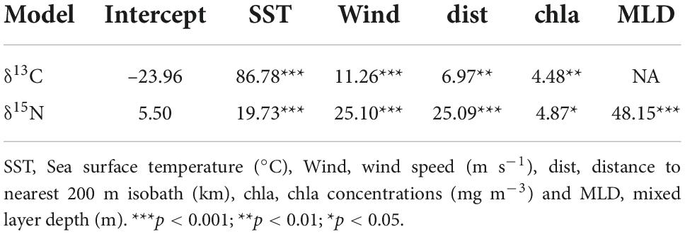
Table 1. Description of the approximate significance of smooth terms for the two selected models (F-values and p-values).
To investigate the overall spatial patterns emerging from yearly δ13C and δ15N isoscapes, we produced maps of average modelled isotopic values for 1998–2020 (Figure 2). North Atlantic zooplankton δ13C isoscapes showed a clear SE to NW gradient with values decreasing northward. South of the North Atlantic current, δ13C values were generally above –22.5‰ and up to about –20‰, while north of the current, δ13C values ranged from –22.5 to –25‰. Isoscapes of δ15N values showed several spots across the study area with high δ15N values over 6‰, including the Gulf Stream area and the southeastern part of the study. Other high spots include an area north of Iceland and two spots near Norwegian and Irish coasts. Lowest δ15N values were found along the east coast of Greenland with a minimum of about 2‰. The variance associated with the predictions was generally higher for δ15N than δ13C. The spatial patterns were otherwise very similar, with higher value observed in area with low sampling coverage and/or environmental conditions at the edge of the initial distribution range.
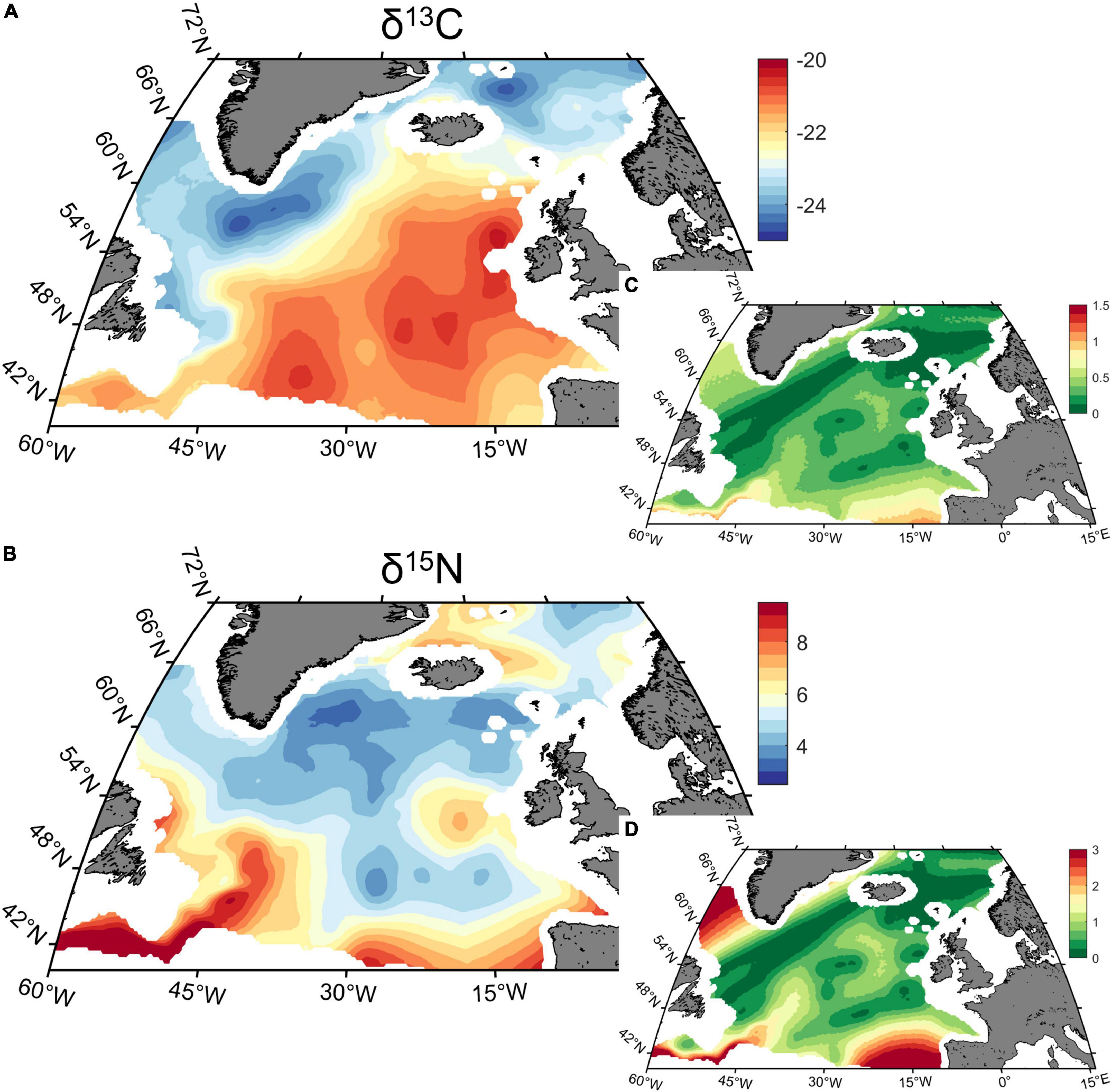
Figure 2. Average of (A) carbon (δ13C) and (B) nitrogen (δ15N) yearly isoscapes (‰) predicted for 1998–2020 in the North Atlantic Ocean, and (C,D) the associated variance of the posterior predicted distribution.
Changes in spatial patterns of zooplankton isotopic composition were also investigated through seasons (Figure 3 and Supplementary Figure 5). Similar to the yearly isoscapes, δ13C values followed a NE to SW gradient, with values covering an identical range. However, the –22.5‰ isoline moves northward from winter to fall. On the other hand, δ15N values increased across the North Atlantic through the seasons, with patches of high values extending significantly.
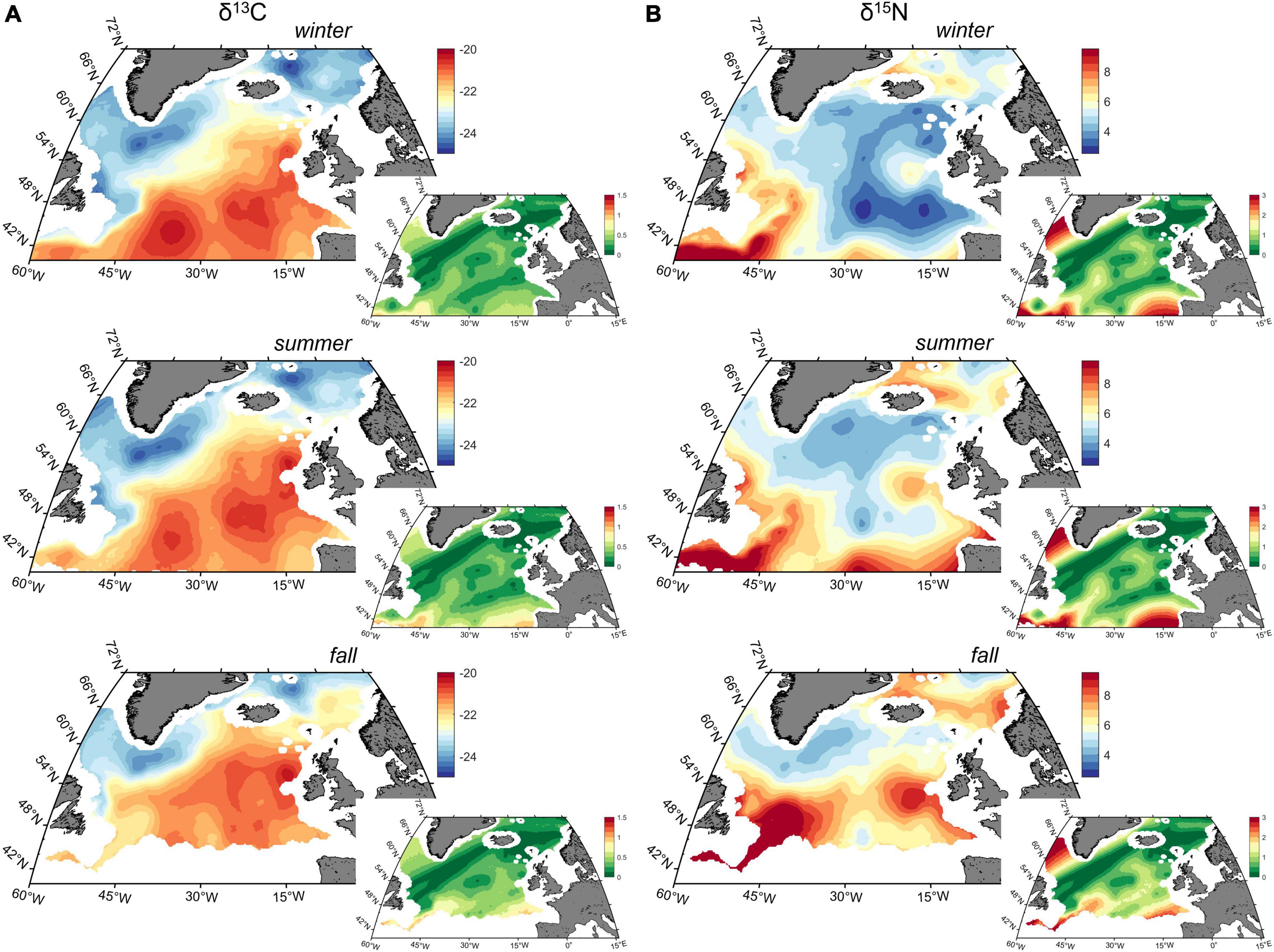
Figure 3. Average of (A) carbon (δ13C) and (B) nitrogen (δ15N) values winter, summer and fall isoscapes (‰) in the North Atlantic Ocean predicted for 1998–2020, and the associated variance of the posterior predicted distribution.
The isoscape trajectory maps highlight the areas characterised by different degrees of variability. To illustrate how the approach works, we chose as an example the variability in δ13C/δ15N isoscapes modelled for 2014 and 2015 (Figure 4).
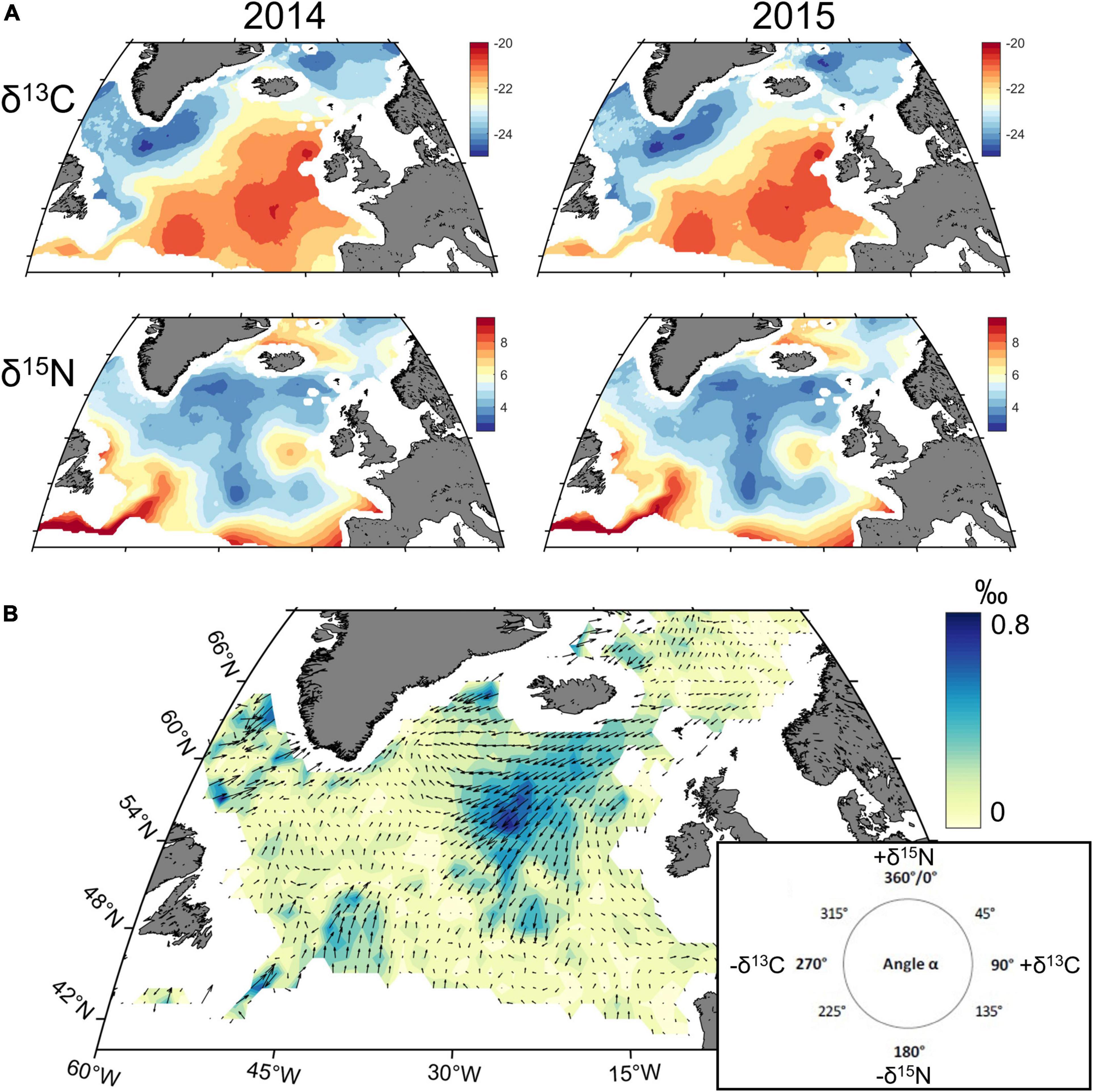
Figure 4. Shift in δ13C/δ15N isoscapes in the North Atlantic Ocean between 2014 and 2015: (A) Isoscape for δ13C/δ15N in 2014 and 2015; (B) Isoscape trajectory map synthetizing the shift for both isotopes between 2014 and 2015. Direction of arrows illustrates direction in the modelled 2D Ωδ space according to increase and/or decrease in δ13C and δ15N values (0–90°: +δ13C and –δ15N; 90–180°: +δ13C and δ15N; 180–270°: –δ13C and –δ15N; 270–360°: –δ13C and +δ15N). Length of arrows and coloured background rasters illustrate modelled trajectory segment length (‰) at each 1° × 1° grid cell.
Trajectory analysis extended to the whole study period identified spatial patterns in the magnitude of yearly isoscape change (Figure 5). Two areas located respectively to the north of Iceland and from the Newfoundland basin extending NE were characterised by the highest trajectory path implying higher short-range spatio-temporal variability in SI compositions.
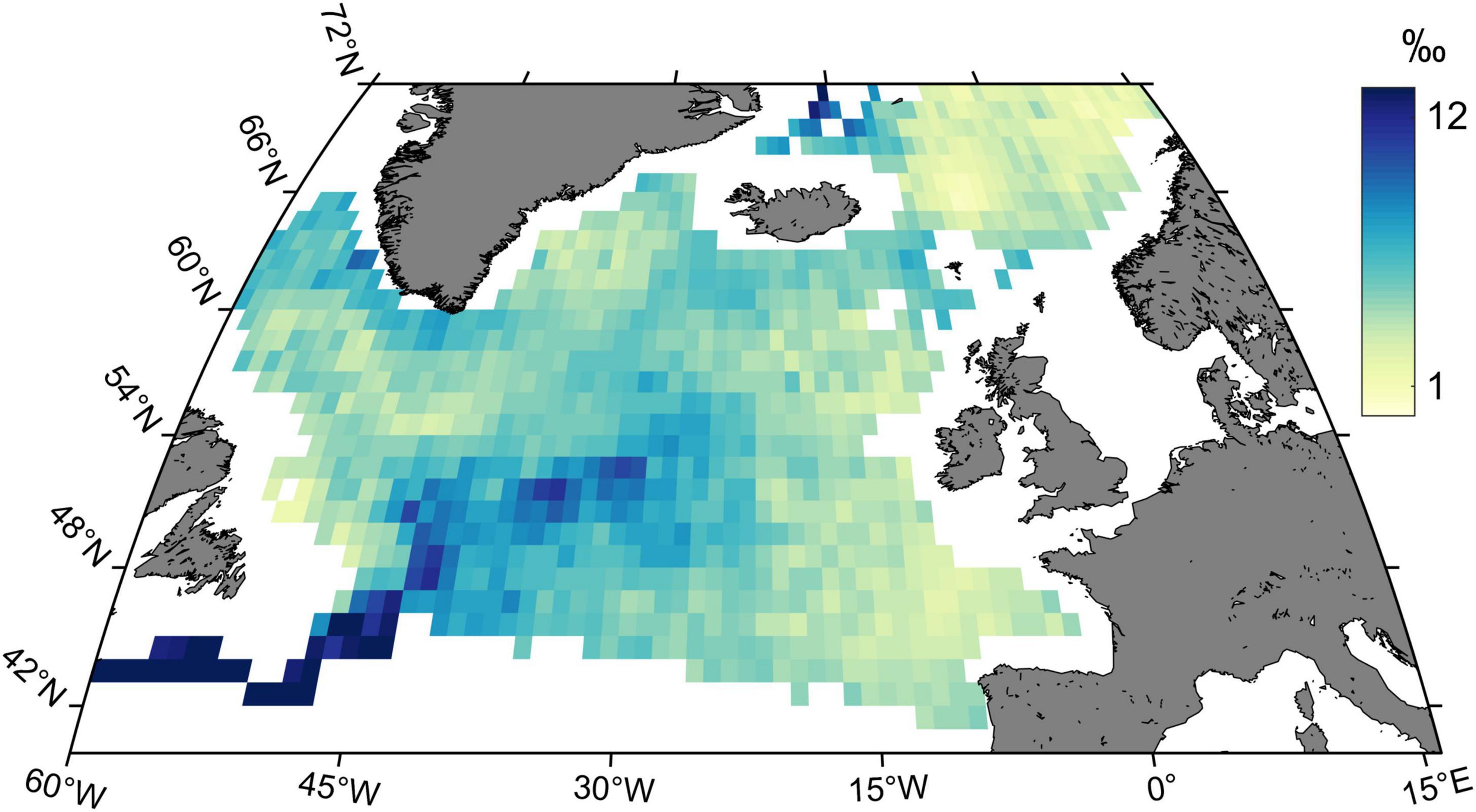
Figure 5. Trajectory map of trajectory path values (‰) for δ13C/δ15N isoscapes in the North Atlantic Ocean from 1998 to 2020. Gradient of colours indicates the spatial trajectory path patterns for each 1° × 1° grid cell.
Results were synthesised in the trajectory heatmap (Figure 6), which pointed out that isoscape dynamics mainly involved direction ranges comprised between 0°and 45°, respectively (i.e., higher δ13C and δ15N values), and 180° and 225° (i.e., lower δ13C and δ15N values). These range of directions indicated that enrichment and depletion were more important for δ15N values than for δ13C values. These two contrasted patterns of both isotopes mainly occurred synchronously in the North Atlantic Ocean suggesting contrasting isoscape dynamics depending on areas. Sporadically, (e.g., 1998–99 and 2008–09), one main pattern characterised by important 15N depletions and slight 13C depletions was observed. An inverse dynamic (i.e., higher δ13C and δ15N values) was observed between 2005 and 2006. In some periods, a more homogenous distribution of the number of stations in the different direction ranges suggested no obvious pattern of isotope dynamics at the scale of the North Atlantic Ocean (e.g., periods 2010–2011 and 2019–2020).
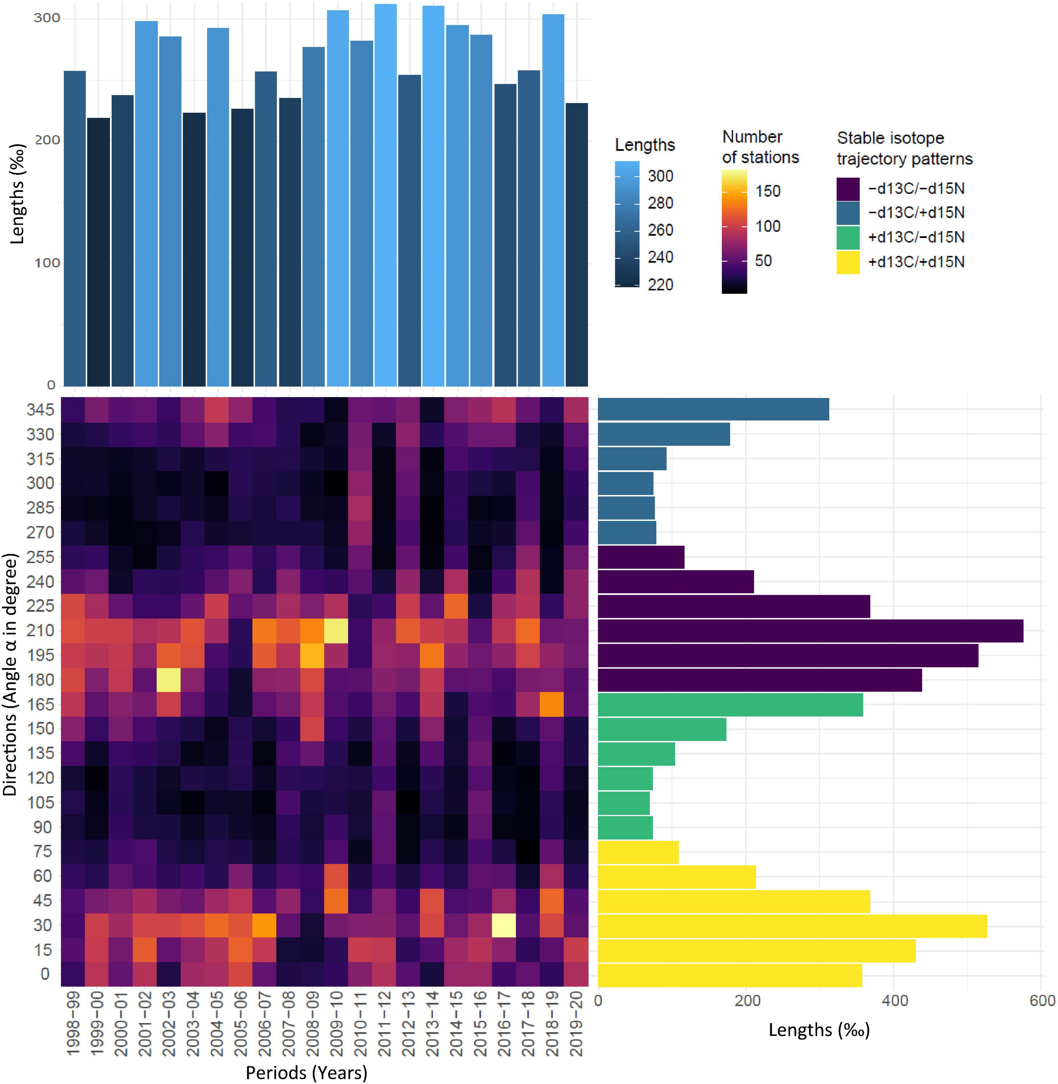
Figure 6. Trajectory heatmap. Heatmap panel: Angles α in the modelled 2D Ωδ space exhibited by all stations within all pairs of dates (1998–1999,…, 2019–2020) are represented by range of direction (15° segments) according to period. Colour gradient from dark blue to yellow indicate the number of stations exhibited by a given range of direction within a given period. X barplot: Sum of segment lengths (‰) across stations and times, exhibiting the chosen range of direction. The blue gradient indicates the magnitude of the sum of segment lengths. Y barplot: Sum of segment lengths according to range of directions. Bars are coloured according to increase and/or decrease in δ13C and δ15N values.
Hierarchical cluster analysis identified five main trajectory clusters characterised by differences in δ13C and δ15N values and SITA metrics (Figure 7 and Supplementary Figure 6). Interestingly, the spatial representation of these clusters (hereafter isoregions) described different well-defined regions at the scale of North Atlantic Ocean (Figure 8). For instance, isoregion #1 exhibited among the highest δ13C/δ15N values and distance-based trajectory metrics values (Figures 7, 9 and Table 2) and grid cells assigned to isoregion #1 were located in constrained areas close to the coast (Figure 8), contrasting with the lower δ15N values and the broader distribution of isoregion #5. Similarly, the nature of changes varied among isoregions (i.e., trajectory segment directions, Figure 9). Results of the Herman and Rasson test confirmed that the trajectory segment directions were not evenly distributed in the 2D Ωδ space (p < 0.001), implying particular enrichment and depletion patterns of both isotopes. Additionally, the Watson–William’ two tests evidenced contrasts in the nature of change between isoregions (Figure 9 and Supplementary Table 3): (1) While isoregion #1 involved direction in the δ13C/δ15N 2D space that mainly characterised patterns of 15N enrichment and depletion, such patterns were more balanced for both isotopes especially in isoregions #2, #3, and #4; (2) At finest scale, the distribution of less abundant direction occurring in an orthogonal way compared to the main directions patterns also varied among isoregions.
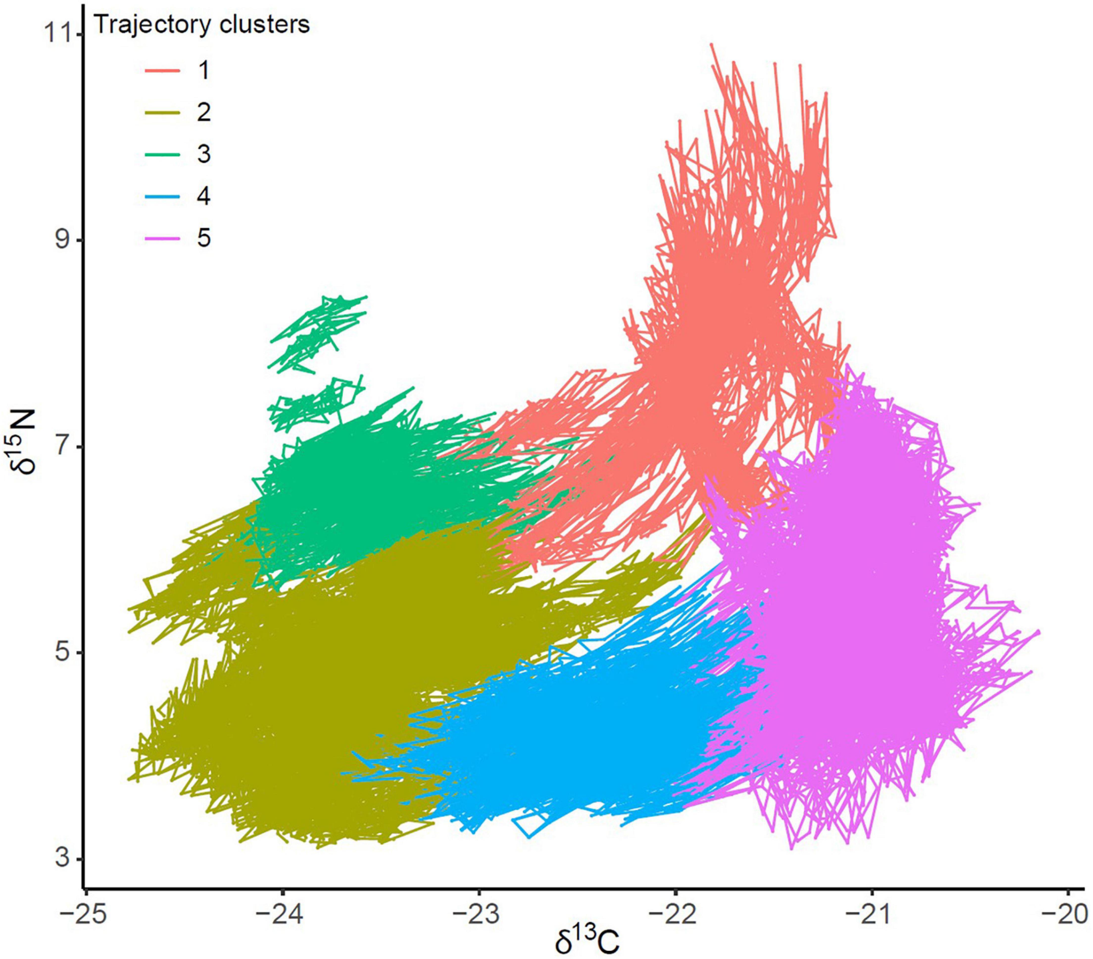
Figure 7. Trajectories of δ13C and δ15N predicted values (‰) at each grid cell for which values were predicted continuously for 1998–2020. Points are coloured according to the five clusters identified by the dissimilarities analyses between trajectories, and chronologically connected for consecutive grid cell values (1998–2020).
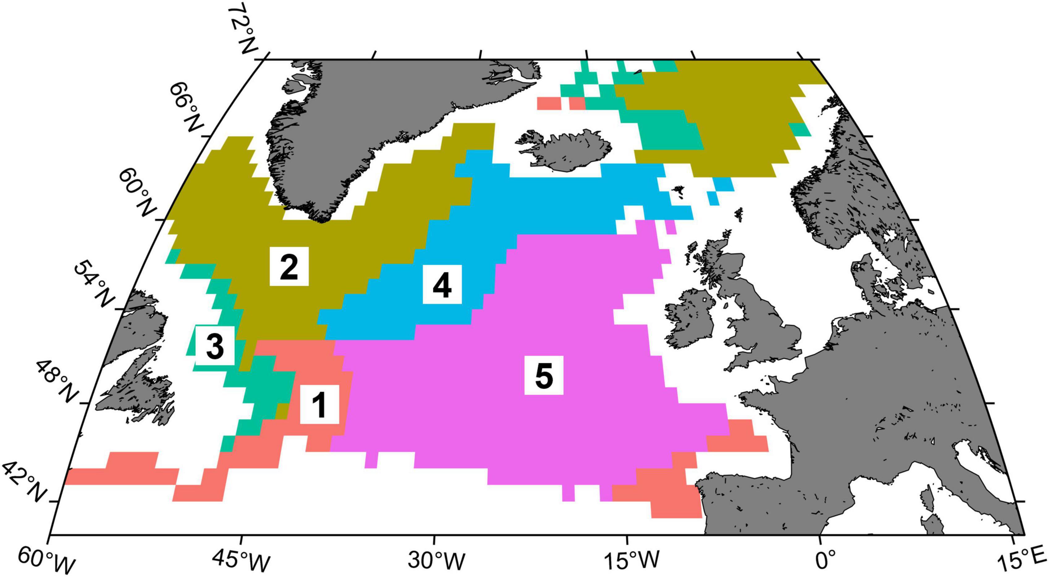
Figure 8. Distribution of the clusters/isoregions defined using all δ13C and δ15N predicted values for 1998–2020 in the North Atlantic Ocean.
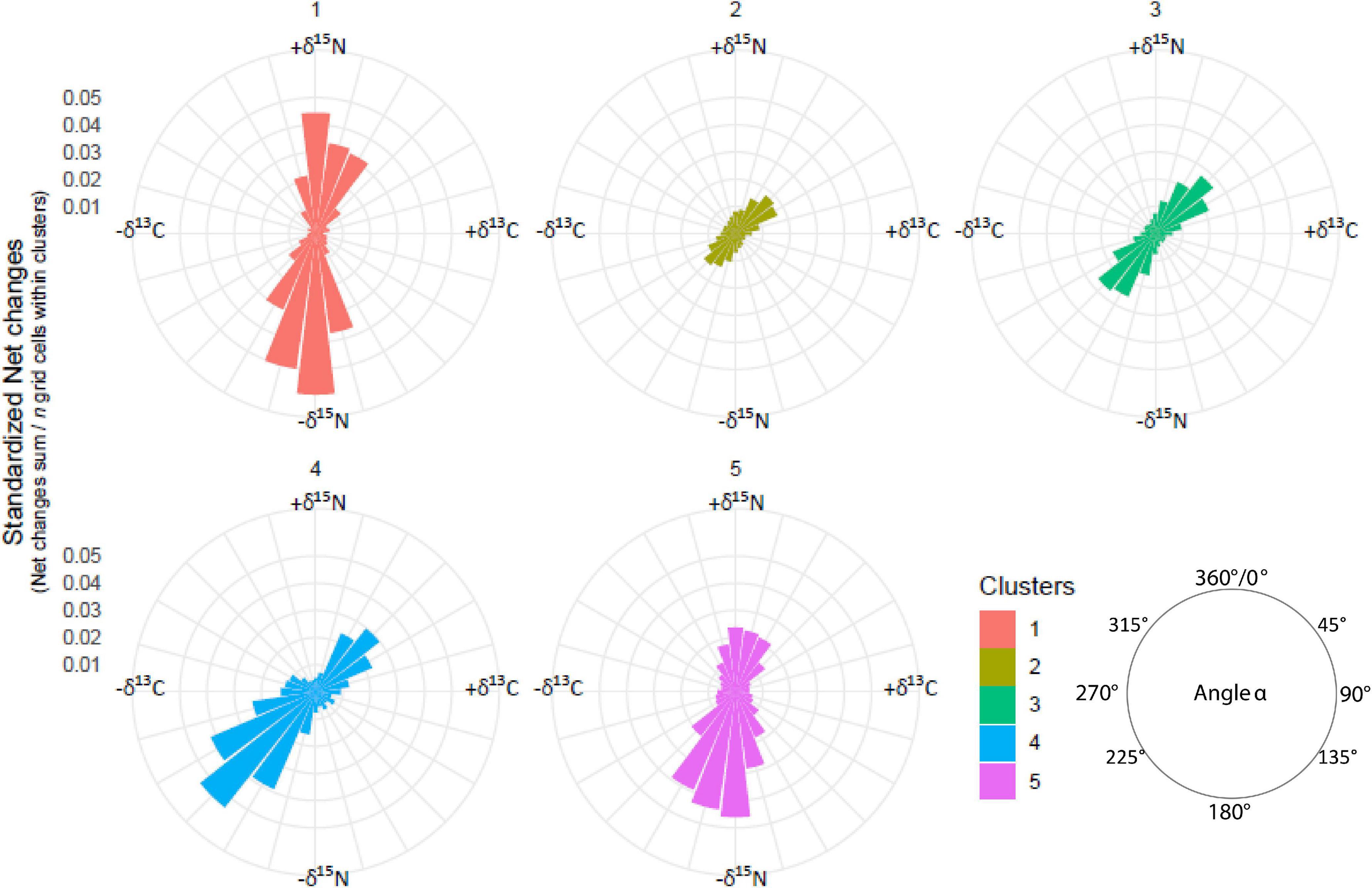
Figure 9. Trajectory direction (0–360°) in the modelled 2D Ωδ space for the five isoregions according to increase and/or decrease in δ13C and δ15N values.
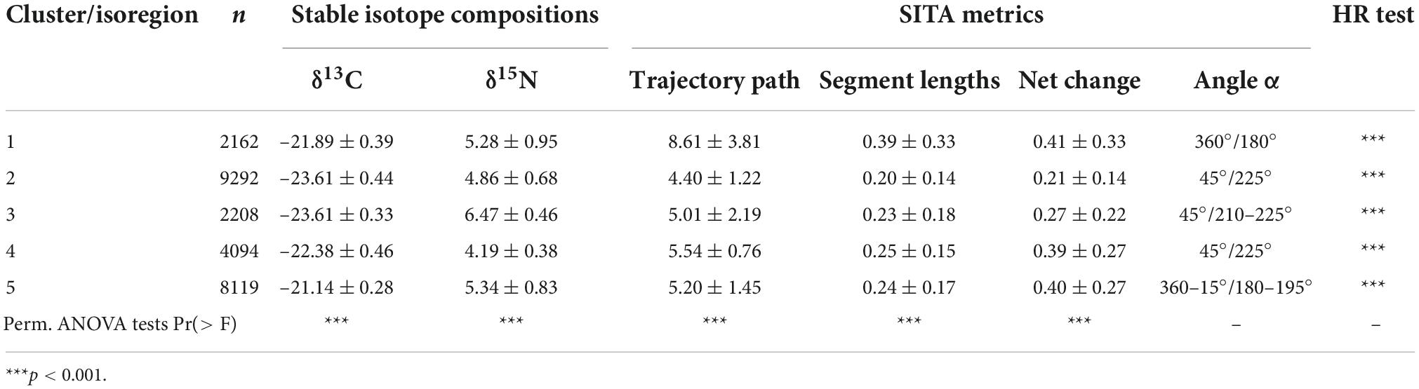
Table 2. Synthesis of δ13C and δ15N values (‰) and SITA length-based (‰) and direction-based (°) metrics for each trajectory clusters/isoregions with respective results of ANOVA permutation tests for stable isotope compositions and length-based metrics, and Herman–Rasson tests for direction-based metrics.
The net changes metric was used to assess temporal trend by comparing isoscape values to a reference, in our case the beginning of the time series, the 1998’s isoscape. Potential year cycles were evidenced, especially for isoregions #4 and #5 also characterised by an increasing trend in net change values (Figure 10). At seasonal scales, cycles were evidenced when looking at the 69 successive isoscapes including all seasons*years from winter 1998 to fall 2020. All isoregions exhibited a cycle characterised by increasing net changes between summer and fall isoscapes followed by a winter reset (Figure 11A). Interestingly, some contrasts were observed in net changes values that characterised changes between winter 1998 and all other seasons. These values were higher for isoregions #1, #3, and #5, compared to isoregions #2 and #3, suggesting differences in the temporality of seasonal dynamics in the North Atlantic Ocean (Figure 11B).
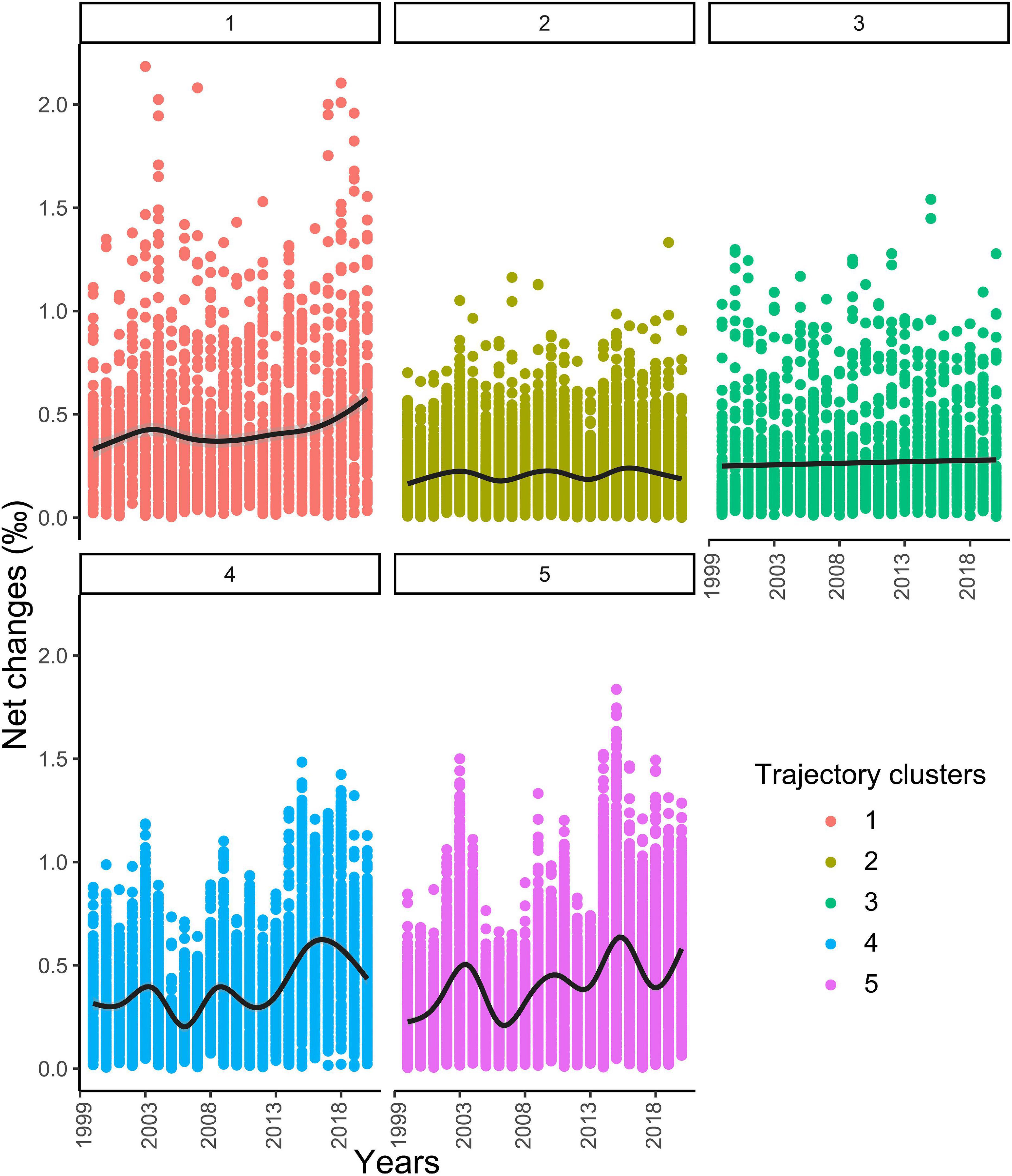
Figure 10. Temporal evolution of the isotopic net changes (‰) for the five isoregions over 1998–2020, taking 1998 as a year of reference. A smoothing line is shown (black thick line).
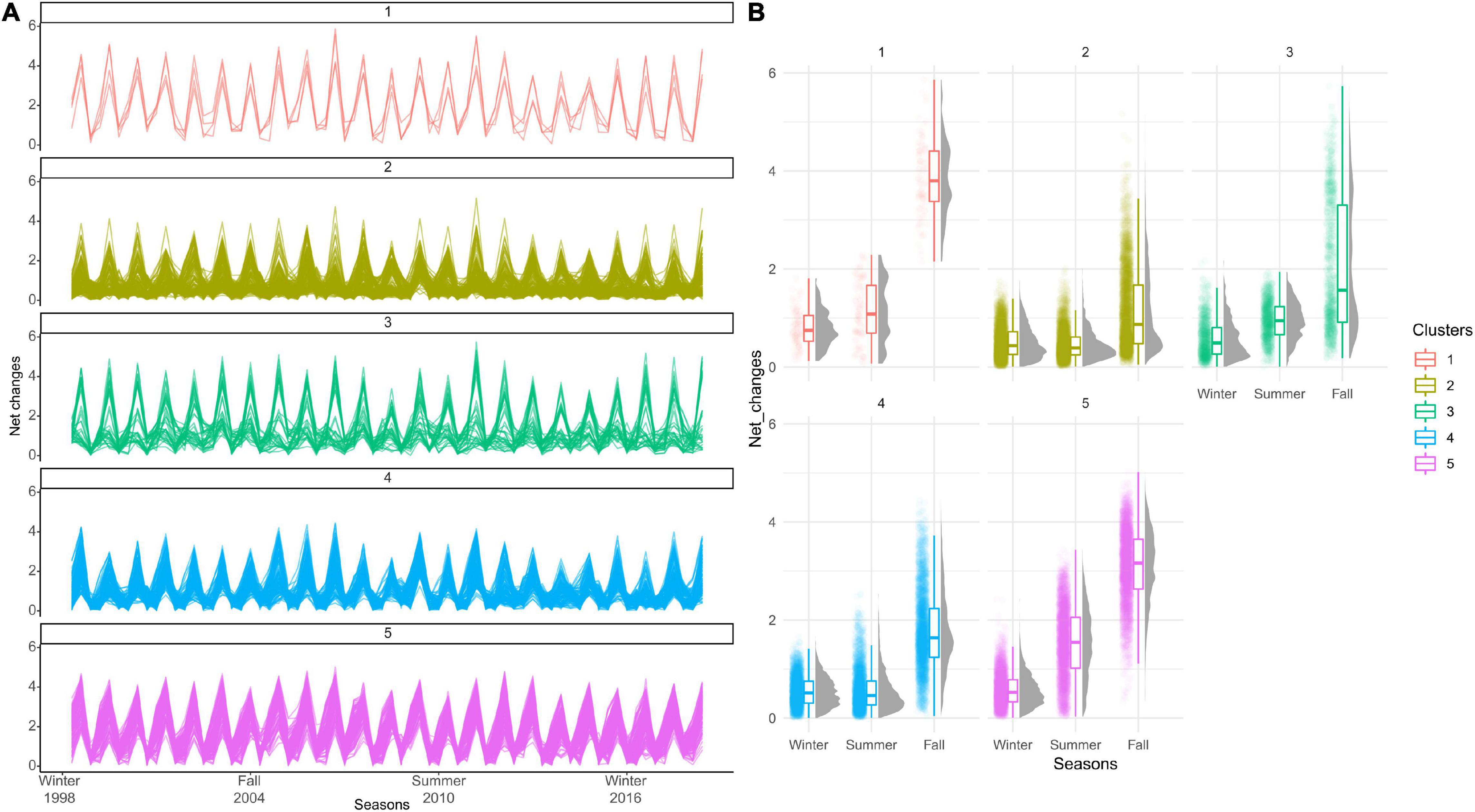
Figure 11. Seasonal isoscape cycles. (A) Temporal evolution of the isotopic net changes (‰) in the five isoregions for the 69 successive isoscapes including all seasons*years from winter 1998 to fall. (B) Box plots of net changes values (‰) exhibits by each trajectory cluster compared to winter 1998.
Discussion
This study provides the first North Atlantic observation-based and time-resolved C and N isoscapes developed using environmental predictors. We modelled δ13C and δ15N isoscapes for three seasons over a time period of 23 years (1998–2020). This effort was made possible thanks to the CPR survey, which collects plankton samples routinely across the entire basin. In the first part of the discussion, we discuss the main drivers of spatio-temporal variation in zooplankton SI compositions in open ocean, firstly at the scale of the North Atlantic basin, then at regional scales. In the second part, we discuss methodological aspects and limitations associated with isoscapes development and use. Finally, we describe the potential of isoscapes in moving forward predator studies.
Potential drivers underpinning spatio-temporal variation in zooplankton isotope compositions
The yearly modelled δ13C values showed two distinct areas, broadly separated by the North Atlantic Current (NAC). δ13C values higher than c. –22.5‰ are likely to originate from the south-eastern region while lower values are associated with the NW area. In the open ocean, temperature is a primary covariate of δ13C variability in phytoplankton. The extent of fractionation of carbon isotopes during photosynthetic fixation by phytoplankton depends on the concentration of CO2 outside of the cell relative to the carbon demand of the cell (Popp et al., 1999; Hofmann et al., 2000; Laws et al., 2002). Increasing temperatures therefore reduce the extent of fractionation (and increase phytoplankton δ13C values) through reductions in solubility of CO2 coupled with increases in cell CO2 demand associated with higher growth rates. The water temperature distribution in the North Atlantic Ocean is determined by the northward flow of warm water transported by the North Atlantic Current which delimits tropical to temperate and subpolar waters. SST was the most powerful covariate in the δ13C model and, as expected, the isoscapes follow this spatial pattern. Other processes, such as influence of coastal waters or intense blooms (Deuser, 1970), also affect δ13C values locally in the open ocean and might explain mesoscale features. Seasonal, temperature-associated isotope patterns identified in the INLA models include a trend of increasing δ13C values potentially associated with water warming from winter through to fall periods. These trends are especially pronounced south of Iceland and in the Norwegian Sea.
The spatial distribution of δ15N values in marine phytoplankton is strongly influenced by nitrate availability and associated variations in isotopically distinct sources of nitrogen taken up by phytoplankton. As with CO2, phytoplankton preferentially use the light NO3– molecule (14N vs. 15N) resulting in δ15N values varying conversely with nitrate concentrations (Rau et al., 1998; Rolff, 2000). In turn, nitrate concentrations are set by the balance between phytoplankton uptake and replenishment via exchanges with underneath water layer. Therefore, chla concentrations and mixed layer depth are important variables in defining δ15N values. High δ15N values occur in productive areas where conditions allow phytoplankton to develop and deplete nitrates (water stability in the surface layer). In addition to the southern part of the study area, i.e., the Gulf Stream area and the Iberian coast, three discrete regions of relatively high δ15N values were identified, north of Iceland, the Norwegian Sea and offshore of the Irish coast.
Ecoregions
Interannual variations and temporal trends in SI values within a study area can be driven either by changes in the productivity/physical regime occurring in the core of the region or by intrusion of waters with distinct nutrient or plankton isotopic composition from adjacent regions. In this study, trajectory analysis implied that enrichment and depletion patterns of both modelled isotopes occurred simultaneously in the North Atlantic Ocean. This is in accordance with St John Glew et al. (2021) results at the scale of the Southern Ocean, but contrasted with Espinasse et al. (2020a) and (Sturbois et al., 2021a) who found that trajectories characterised by increases in δ13C and δ15N values alternated with decreases in both isotope values at the smallest scale of the Northeast Pacific. They showed that the level of intrusion of sub-tropical waters transporting zooplankton with higher isotopic values was the main driver of alternation between high and low SI values as represented by the SITA heatmap (Sturbois et al., 2021a). In this work, we show how large spatio-temporal scale isoscape modelling approaches can provide insight into local patterns and processes under the influence of environmental drivers, and the need to partition the study area in distinct isotopic regions.
Definitions of habitats, bioregions or ecoregions have been a useful tool to partition the ocean realm (Longhurst, 2010) and were recently updated for the North Atlantic Ocean (Beaugrand et al., 2019). The five isoregions defined in this study can be classified as follows: #1 and #3 potential coastal influence; #2 and #4 polar and sub-polar areas, respectively, part of the polar biome as defined by Longhurst (2010); #5 area south to the Gulf Stream/North Atlantic current, classified as Westerly Wind biome in Longhurst (2010). Isoregions #1 and #3 are distributed along continental shelves and are both likely to be influenced by coastal waters. Coastal/offshore water exchanges and associated plankton communities can be promoted by winds, eddies or freshwater runoff (Mackas and Coyle, 2005). Coastal waters usually transport zooplankton with specific isotopic values, which are generally higher than offshore, as these areas are often continuously productive (Kline, 2009; El-Sabaawi et al., 2013). The western distribution of the isoregion #1 corresponds roughly to the ecology unit Gulf Stream Extension, while its eastern part corresponds to Pseudo-oceanic warm-temperate, as defined by Beaugrand et al. (2019; see Supplementary Figure 7). They represent a mix of offshore and coastal waters and are influenced by subtropical climate. Isoregion #3 corresponds to the ecological unit Polar Shelf Edge, which is characterised by cold water, high chla concentrations and intermediate nitrate levels. Isoregions #2 and #4 corresponds to the ecological unit Polar Oceanic and Sub-Polar Oceanic, respectively. Both ecological units are characterised by cold waters and high nitrate concentrations. Isoregion #5 corresponds to ecological unit Oceanic Warm Temperate and Diverse and Productive Oceanic Temperate, characterised by warm waters and intermediate nitrate level. Overall, the temperature and nitrates concentrations between the isoregions/ecological units vary accordingly with the levels of δ13C and δ15N values, with expected similar trends between temperature and δ13C and opposite trends between nitrates concentrations and δ15N values.
Temporal trends
Interesting oscillating patterns in the intensity of changes were observed for some of the isoregions. The oscillations in the isoregions #4 and #5 showed a certain degree of synchronicity over the time period studied (Figure 10). The strength of the NAC is a natural candidate to explain these fluctuations. The NAC transports heat from the south to the eastern part of the North Atlantic and the recent weakening of the Atlantic meridional overturning circulation (AMOC) has led to negative temperature anomalies in the east part of the North Atlantic (Caesar et al., 2018). The fluctuations in net changes observed in these isoregions follow temperature anomalies recorded for these areas. These anomalies are driven by the balance between the relative proportion of water originating from sub tropical or sub polar areas (Desbruyères et al., 2021). It is interesting to note that δ13C and δ15N values vary together in isoregions #2 and #4, while there is a decoupling in the isoregion #5, for which mainly δ15N values vary. Temperature changes in sub polar and polar waters (isoregions #2 and #4) are likely to influence both isotopic ratios, directly in the case of δ13C and via an increase in stratification for δ15N. In isoregion #5, change in the North Atlantic Oscillation and associated wind regime might play a major role by affecting the MLD and indirectly the δ15N values (Hurrell and Deser, 2009).
Model structure and isoscape limitations
Modelling isotopic values over large areas implies some constraints. Notably, the isoscapes should preferentially be based on consistent observational data, i.e., isotopic compositions of materials or organisms that belong to similar trophic level, and these individuals should be situated low enough in the food webs that most predators can be compared to them. Particulate organic matter (Kurle and Mcwhorter, 2017; Seyboth et al., 2018; St John Glew et al., 2021), jellyfish (Mackenzie et al., 2014; St John Glew et al., 2019), zooplankton composition or individuals (Brault et al., 2018; Espinasse et al., 2020b; Matsubayashi et al., 2020) have been used in previous studies to produce large spatial scale isoscapes. A balance needs to be found between the quality (spatiotemporal resolution, consistence in analysing, and sampling procedure among samples) and the quantity of data. In this study, the CPR survey provided us with excellent quality species specific samples with relatively high sample numbers providing reasonable, but not random, spatiotemporal coverage. Furthermore, the tissue turnover rates for copepods (ca 2 weeks) (Graeve et al., 2005; Tiselius and Fransson, 2016), acting as a smoothing buffer, help to match predictor and isotopic values and to create more stable isoscapes. Although the CPR survey samples copepods close to the surface, Calanus are known to undergo diel vertical migration (Dale and Kaartvedt, 2000), and can feed on prey distributed at different depths, integrating SI values along the water column. Particulate organic matter, despite its highly dynamic isotopic composition, represents a good alternative having the advantage of samples being generally available in greater number. Using SI data from higher trophic level animals such as small pelagic fish as a reference is also another option, but data are usually limited, and assumptions of true geolocation may be violated. Defining a “perfect” tissue to generate geo-referenced data supporting isoscape model development is challenging. However, a strong advantage of the Bayesian INLA framework used here to construct spatial models is that it allows the user to define and partition non-spatial sources of variance in isotope values, and to retrieve spatial uncertainties associated with source effects (St John Glew et al., 2019).
The variability in observed (measured) isotope data was expectedly greater than in modelled data. This implies that sources of variation were higher than the models capture. Some of the processes involved in setting and transferring the SI values along the trophic chain are difficult to translate into the model formulation (e.g., phytoplankton composition and cell geometry). However, the predictors selected during the model formation are sufficient to capture the main processes driving isotopic variations. It is relatively straight forward to model spatio-temporal variations in δ13C values, as SST is a strong proxy for both CO2 concentration and isotopic fractionation. SST data are available at high spatio-temporal resolution allowing effective prediction across unsampled regions. By contrast, nitrate concentrations, the main driver of variations in δ15N values, are harder to resolve from remote sensed data. Chla concentrations derived from ocean colour data are an obvious alternative candidate, but complex phytoplankton dynamics and limits associated with measurements (surface layer only) weakens the relationship. Among the different hypotheses on mechanisms controlling phytoplankton dynamics (Behrenfeld and Boss, 2014; Lindemann and St. John, 2014) and bloom initiation (Mahadevan et al., 2012), the mix layer depth recurrently plays an important role. It might explain why MLD was found to be a more powerful predictor than chla to model δ15N values (Table 1).
Overall the systematic and logically reasonable patterns observed in the modelled isoscapes make us confident of their consistency, however limited data are available to compare our isoscape values at regional scales. We compared our mean zooplankton modelled δ13C values per isoregion (Table 2) with a review of previous observational data per Longhurst bioregion produced by Magozzi et al. (2017). Values were found to be consistent with –23.6 vs. –23.4‰ for the isoregion #2 vs. polar biome, –22.4 vs. –23.7‰ for the isoregion #2 vs. the subpolar biome and –21.1 vs. –21.3‰ for the isoregion #5 vs. Westerly Wind biome.
Caution should be taken when using isoscapes values associated with high uncertainties values (i.e., high variances), particularly when drawing on isoscapes to infer aspects of predator ecology. Two main factors promote high uncertainties in predicted data, spatial segregation from observational data and extreme predictor values. A combination of both can lead to high uncertainties, as can be seen in the southeastern area of the δ15N isoscapes (Figures 3, 4). Accuracy in predicted data far away from observation will depend on distance to the nearest observation, mesh shape/resolution and correlation length distance. We aimed to find a compromise between isoscape resolution and data uncertainties as to keep the latter in reasonable range (ca 1.5‰ for δ13C and 3‰ for δ15N). Extreme predicator values are a problem toward the limits of the domain (e.g., warm water in the south border) and this problem is amplified within the more data-limited seasonal isoscapes. To reduce the uncertainties more observational should be added to the model, ideally coming from undersampled regions and/or during extreme events.
The models we developed could easily be updated in the future by integrating other datasets, still keeping a control on the accuracy of the predictions. Building a larger data base (see for example Verwega et al., 2021) would enable us to develop further the seasonal isoscape, in terms of coverage but also of model structures (e.g., to test specific seasonal model structure). Regarding seasonality, δ13C and δ15N values might vary asynchronously and will not necessarily share the same model structure. In this study, we modelled spatial variances using all-seasons data and produced seasonal isoscapes using seasonal predictors (environmental variables). Our approach assumes that the statistical relationship between the response variable and the predictors do not change over seasons. This is likely largely true for δ13C values where temperature is a strong indirect driver, but it is less clear for δ15N values. Developing fully seasonally specific models would be particularly interesting for δ15N, where the value for one season can potentially be influenced by what happened previously during the year. There is a stronger seasonal pattern in δ15N values, as in contrast to δ13C values the limiting molecule (CO2 vs. nitrates), is only replenished over winter. Fall isotopic composition of copepods will therefore be influenced by the strength of the fall bloom but also potentially of the spring bloom.
Implications for predator movements and trophic interactions
Spatio-temporal patterns in isoscapes have strong implications for the study of food web and animal movements in space and time (Graham et al., 2010; McMahon et al., 2013b; Trueman and St John Glew, 2019). Our study has direct applications for the interpretation consumer stable isotope values in the North Atlantic Ocean where isoregions exhibited contrasting spatio-temporal patterns in modelled isoscapes. The yearly and seasonal dynamics in stable isotope values inferred offers the possibility to investigate predator dynamics at different temporal scales depending on their life cycles. Stable isotope compositions can be measured in a wide range of tissues with different characteristics in terms of turnover rates and growth structures. For example, considering marine mammals, incrementally grown tissues such as seal whiskers, fish eye lenses, baleen plates or seal teeth allow for the description of seasonal, annual or multi-annual resolution (Kernaléguen et al., 2012; Borrell et al., 2013; Trueman et al., 2019; De La Vega et al., 2022). Among other top predators, the practical potential for drawing valuable inferences from tissue isotopes informed from ocean-basin isoscapes is particularly high for species which spend a large part of their life cycle in open ocean but migrate occasionally to coastal areas where they are accessible for sampling (e.g., central point breeding seabirds, and marine mammals, or fish with coastally or freshwater directed spawning such as salmon; e.g., Mackenzie et al., 2011; Trueman et al., 2012; Cherel et al., 2016). Quantifying likely scales of temporal variance in baseline stable isotope values is especially important, particularly where tissues sampled reflect a discrete time period, or where studies draw on time series or compile data across multiple sampling years or seasons. Variation in consumer tissue isotope values is caused by spatio-temporal variation in the isotopic composition of the dietary baseline, differences in diet organisms (including trophic level) and physiological differences in the extent of isotopic spacing between tissue and diet. The potentially confounding effect of these processes can be mitigated by analysing stable isotope compositions of individual amino acids. Essential (source) amino acids are considered to reflect the isotopic composition of primary production conserved through food webs (e.g., Chikaraishi et al., 2009). The isoscapes presented here describe expected spatio-temporal variations in baseline isotope compositions as expressed in bulk protein, and absolute differences among regions are likely to be more pronounced in amino acids such as phenylalanine. Drawing on individual amino acid data may therefore improve accuracy of spatial assignment (Matsubayashi et al., 2020). Such helpful information should be coupled with a strong knowledge of consumers ecology and isotopic integration time (Possamai et al., 2021), other biogeochemical tracers in complementary tissues (Vander Zanden et al., 2016) and, when possible, telemetry data in order to disentangle dynamics in SI compositions due to migrations or changes in feeding strategy (Cherel et al., 2016). Knowledge in spatial niche arrangement of top predators at large scale is necessary to develop conservation measures such as Marine Protected Areas (Reisinger et al., 2022). The isoscapes presented here are provided in the hope that they may help to improve our understanding of poorly documented parts of migratory marine species’ life cycles, many of which have seen their population decline dramatically over the last decades (e.g., Dias et al., 2019).
Data availability statement
Observational stable isotope data as well as the isoscapes and variance predictions produced in the present study are available at https://github.com/borisespinasse/ISOSCAPE_NA. Further queries should be directed to the corresponding author.
Author contributions
BE, SB, and CT conceived the project. PH and DJ provided the access to new materials (zooplankton). JN analysed the samples for stable isotope values. BE developed the spatial Bayesian models to produce the isoscapes. BE and AS carried out the data analysis and wrote the manuscript. All authors provided the editorial advice, and read and approved the final manuscript.
Funding
The CPR Survey would not be possible without the support of the shipping industry, nor the dedication of the past and present team. Current funding includes the UK Natural Environment Research Council, Grant/Award Numbers: NE/R002738/1 and NE/M007855/1; EMFF; Climate Linked Atlantic Sector Science, Grant/Award Number: NE/R015953/1, DEFRA UK ME-5308, NSF USA OCE-1657887, DFO CA F5955-150026/001/HAL, NERC UK NC-R8/H12/100, Horizon 2020: 862428 Mission Atlantic and AtlantECO 862923, IMR Norway and the French Ministry of Environment, Energy, and the Sea (MEEM). Stable isotope measurements were funded by a National Environmental Isotope Facility grant-in-kind (no. 2323) to CT and BE. BE was funded from the European Union’s Horizon 2020 MSCA program under Grant agreement no. 894296 – Project ISOMOD.
Conflict of interest
The authors declare that the research was conducted in the absence of any commercial or financial relationships that could be construed as a potential conflict of interest.
Publisher’s note
All claims expressed in this article are solely those of the authors and do not necessarily represent those of their affiliated organizations, or those of the publisher, the editors and the reviewers. Any product that may be evaluated in this article, or claim that may be made by its manufacturer, is not guaranteed or endorsed by the publisher.
Supplementary material
The Supplementary Material for this article can be found online at: https://www.frontiersin.org/articles/10.3389/fevo.2022.986082/full#supplementary-material
Footnotes
References
Akaike, H. (1974). A new look at the statistical model identification. IEEE Trans. Autom. Control 19, 716–723. doi: 10.1109/TAC.1974.1100705
Batten, S. D., Clark, R., Flinkman, J., Hays, G., John, E., John, A. W. G., et al. (2003). CPR sampling: The technical background, materials and methods, consistency and comparability. Prog. Oceanogr. 58, 193–215. doi: 10.1016/j.pocean.2003.08.004
Beaugrand, G., Brander, K. M., Alistair Lindley, J., Souissi, S., and Reid, P. C. (2003). Plankton effect on cod recruitment in the North Sea. Nature 426, 661–664. doi: 10.1038/nature02164
Beaugrand, G., Edwards, M., and Hélaouët, P. (2019). An ecological partition of the Atlantic Ocean and its adjacent seas. Prog. Oceanogr. 173, 86–102. doi: 10.1016/j.pocean.2019.02.014
Behrenfeld, M. J., and Boss, E. S. (2014). Resurrecting the ecological underpinnings of ocean plankton blooms. Annu. Rev. Mar. Sci. 6, 167–194. doi: 10.1146/annurev-marine-052913-021325
Behrenfeld, M. J., and Falkowski, P. G. (1997). Photosynthetic rates derived from satellite-based chlorophyll concentration. Limnol. Oceanogr. 42, 1–20. doi: 10.4319/lo.1997.42.1.0001
Bicknell, A. W. J., Campbell, M., Knight, M. E., Bilton, D. T., Newton, J., and Votier, S. C. (2011). Effects of formalin preservation on stable carbon and nitrogen isotope signatures in calanoid copepods: Implications for the use of continuous plankton recorder survey samples in stable isotope analyses. Rapid Commun. Mass Spectrom. 25, 1794–1800. doi: 10.1002/rcm.5049
Borrell, A., Velásquez Vacca, A., Pinela, A. M., Kinze, C., Lockyer, C. H., Vighi, M., et al. (2013). Stable isotopes provide insight into population structure and segregation in eastern North Atlantic sperm whales. PLoS One 8:e82398. doi: 10.1371/journal.pone.0082398
Bowen, G. J. (2010). Isoscapes: Spatial pattern in isotopic biogeochemistry. Annu. Rev. Earth Planet. Sci. 38, 161–187. doi: 10.1146/annurev-earth-040809-152429
Brault, E. K., Koch, P. L., Mcmahon, K. W., Broach, K. H., Rosenfield, A. P., Sauthoff, W., et al. (2018). Carbon and nitrogen zooplankton isoscapes in West Antarctica reflect oceanographic transitions. Mar. Ecol. Prog. Ser. 593, 29–45. doi: 10.3354/meps12524
Brun, P., Stamieszkin, K., Visser, A. W., Licandro, P., Payne, M. R., and Kiørboe, T. (2019). Climate change has altered zooplankton-fuelled carbon export in the North Atlantic. Nat. Ecol. Evol. 3, 416–423. doi: 10.1038/s41559-018-0780-3
Buchanan, P. J., Tagliabue, A., De La Vega, C., and Mahaffey, C. (2021). Oceanographic and biogeochemical drivers cause divergent trends in the nitrogen isoscape in a changing Arctic Ocean. Ambio 51, 383–397. doi: 10.1007/s13280-021-01635-6
Bundy, A., Renaud, P. E., Coll, M., Koenigstein, S., Niiranen, S., Pennino, M. G., et al. (2021). Editorial: Managing for the future: Challenges and approaches for disentangling the relative roles of environmental change and fishing in marine ecosystems. Front. Mar. Sci. 8:753459. doi: 10.3389/fmars.2021.753459
Caesar, L., Rahmstorf, S., Robinson, A., Feulner, G., and Saba, V. (2018). Observed fingerprint of a weakening Atlantic Ocean overturning circulation. Nature 556, 191–196. doi: 10.1038/s41586-018-0006-5
Cherel, Y., and Hobson, K. A. (2007). Geographical variation in carbon stable isotope signatures of marine predators: A tool to investigate their foraging areas in the Southern Ocean. Mar. Ecol. Prog. Ser. 329, 281–287. doi: 10.3354/meps329281
Cherel, Y., Quillfeldt, P., Delord, K., and Weimerskirch, H. (2016). Combination of at-sea activity, geolocation and feather stable isotopes documents where and when seabirds molt. Front. Ecol. Evol. 4:3. doi: 10.3389/fevo.2016.00003
Chikaraishi, Y., Ogawa, N. O., Kashiyama, Y., Takano, Y., Suga, H., Tomitani, A., et al. (2009). Determination of aquatic food-web structure based on compound-specific nitrogen isotopic composition of amino acids. Limnol. Oceanogr. Methods 7, 740–750. doi: 10.4319/lom.2009.7.740
Chivers, W. J., Walne, A. W., and Hays, G. C. (2017). Mismatch between marine plankton range movements and the velocity of climate change. Nat. Commun. 8:14434. doi: 10.1038/ncomms14434
Clark, C. T., Cape, M. R., Shapley, M. D., Mueter, F. J., Finney, B. P., and Misarti, N. (2021). SuessR: Regional corrections for the effects of anthropogenic CO2 on δ13C data from marine organisms. Methods Ecol. Evol. 12, 1508–1520. doi: 10.1111/2041-210X.13622
Coplen, T. B., Brand, W. A., Gehre, M., Gröning, M., Meijer, H. A. J., Toman, B., et al. (2006). New guidelines for δ13C measurements. Anal. Chem. 78, 2439–2441. doi: 10.1021/ac052027c
Cushing, D. H. (1990). “Plankton production and year-class strength in fish populations: An update of the match/mismatch hypothesis,” in Advances in marine biology, Vol. 26, eds J. H. S. Blaxter and A. J. Southward (Cambridge, MA: Academic Press), 249–293. doi: 10.1016/S0065-2881(08)60202-3
Dale, T., and Kaartvedt, S. (2000). Diel patterns in stage-specific vertical migration of Calanus finmarchicus in habitats with midnight sun. ICES J. Mar. Sci. 57, 1800–1818. doi: 10.1006/jmsc.2000.0961
De Cáceres, M., Coll, L., Legendre, P., Allen, R. B., Wiser, S. K., Fortin, M.-J., et al. (2019). Trajectory analysis in community ecology. Ecol. Monogr. 89:e01350. doi: 10.1002/ecm.1350
De La Vega, C., Buchanan, P. J., Tagliabue, A., Hopkins, J. E., Jeffreys, R. M., Frie, A. K., et al. (2022). Multi-decadal environmental change in the Barents Sea recorded by seal teeth. Glob. Change Biol. 28, 3054–3065. doi: 10.1111/gcb.16138
Desbruyères, D., Chafik, L., and Maze, G. (2021). A shift in the ocean circulation has warmed the subpolar North Atlantic Ocean since 2016. Commun. Earth Environ. 2:48. doi: 10.1038/s43247-021-00120-y
Deuser, W. G. (1970). Isotopic evidence for diminishing supply of available carbon during diatom bloom in the Black Sea. Nature 225, 1069–1071. doi: 10.1038/2251069a0
Dias, M. P., Martin, R., Pearmain, E. J., Burfield, I. J., Small, C., Phillips, R. A., et al. (2019). Threats to seabirds: A global assessment. Biol. Conserv. 237, 525–537. doi: 10.1016/j.biocon.2019.06.033
Drinkwater, K. F., Sundby, S., and Wiebe, P. H. (2020). Exploring the hydrography of the boreal/arctic domains of North Atlantic seas: results from the 2013 BASIN survey. Deep Sea Res. Part II: Top. Stud. Oceanograp. 180:104880. doi: 10.1016/j.dsr2.2020.104880
El-Sabaawi, R., Dower, J., Kainz, M., and Mazumder, A. (2009). Characterizing dietary variability and trophic positions of coastal calanoid copepods: Insight from stable isotopes and fatty acids. Mar. Biol. 156, 225–237. doi: 10.1007/s00227-008-1073-1
El-Sabaawi, R., Trudel, M., and Mazumder, A. (2013). Zooplankton stable isotopes as integrators of bottom-up variability in coastal margins: A case study from the Strait of Georgia and adjacent coastal regions. Prog. Oceanogr. 115, 76–89. doi: 10.1016/j.pocean.2013.05.010
Espinasse, B., Harmelin-Vivien, M., Tiano, M., Guilloux, L., and Carlotti, F. (2014). Patterns of variations in C and N stable isotope ratios in size-fractionated zooplankton in the Gulf of Lion, NW Mediterranean Sea. J. Plankton Res. 36, 1204–1215. doi: 10.1093/plankt/fbu043
Espinasse, B., Hunt, B. P. V., Doson Coll, Y., and Pakhomov, E. A. (2018). Investigating high seas foraging conditions for salmon in the North Pacific: Insights from a 100-year scale archive for Rivers Inlet sockeye salmon. Can. J. Fish. Aquat. Sci. 76, 918–927. doi: 10.1139/cjfas-2018-0010
Espinasse, B., Hunt, B. P. V., Batten, S. D., and Pakhomov, E. A. (2020a). Defining isoscapes in the Northeast Pacific as an index of ocean productivity. Glob. Ecol. Biogeogr. 29, 246–261. doi: 10.1111/geb.13022
Espinasse, B., Hunt, B. P. V., Finney, B. P., Fryer, J. K., Bugaev, A. V., and Pakhomov, E. A. (2020b). Using stable isotopes to infer stock-specific high-seas distribution of maturing sockeye salmon in the North Pacific. Ecol. Evol. 10, 13555–13570. doi: 10.1002/ece3.7022
Fitak, R. R., and Johnsen, S. (2017). Bringing the analysis of animal orientation data full circle: Model-based approaches with maximum likelihood. J. Exp. Biol. 220, 3878–3882. doi: 10.1242/jeb.167056
Fuglstad, G.-A., Simpson, D., Lindgren, F., and Rue, H. (2019). Constructing priors that penalize the complexity of Gaussian random fields. J. Am. Stat. Assoc. 114, 445–452. doi: 10.1080/01621459.2017.1415907
Good, S., Fiedler, E., Mao, C., Martin, M. J., Maycock, A., Reid, R., et al. (2020). The current configuration of the OSTIA system for operational production of foundation sea surface temperature and ice concentration analyses. Remote Sens. 12:720. doi: 10.3390/rs12040720
Graeve, M., Albers, C., and Kattner, G. (2005). Assimilation and biosynthesis of lipids in Arctic Calanus species based on feeding experiments with a 13C labelled diatom. J. Exp. Mar. Biol. Ecol. 317, 109–125. doi: 10.1016/j.jembe.2004.11.016
Graham, B. S., Koch, P. L., Newsome, S. D., McMahon, K. W., and Aurioles, D. (2010). “Using isoscapes to trace the movements and foraging behavior of top predators in oceanic ecosystems,” in Isoscapes: Understanding movement, pattern, and process on Earth through isotope mapping, eds J. B. West, G. J. Bowen, T. E. Dawson, and K. P. Tu (Dordrecht: Springer Netherlands), 299–318. doi: 10.1007/978-90-481-3354-3_14
Gruber, N., Keeling, C. D., Bacastow, R. B., Guenther, P. R., Lueker, T. J., Wahlen, M., et al. (1999). Spatiotemporal patterns of carbon-13 in the global surface oceans and the oceanic Suess effect. Glob. Biogeochem. Cycles 13, 307–335. doi: 10.1029/1999GB900019
Gutiérrez-Rodríguez, A., Décima, M., Popp, B. N., and Landry, M. R. (2014). Isotopic invisibility of protozoan trophic steps in marine food webs. Limnol. Oceanogr. 59, 1590–1598. doi: 10.4319/lo.2014.59.5.1590
Halpern, B. S., Frazier, M., Afflerbach, J., Lowndes, J. S., Micheli, F., O’Hara, C., et al. (2019). Recent pace of change in human impact on the world’s ocean. Sci. Rep. 9:11609. doi: 10.1038/s41598-019-47201-9
Hays, G. C., Richardson, A. J., and Robinson, C. (2005). Climate change and marine plankton. Trends Ecol. Evol. 20, 337–344. doi: 10.1016/j.tree.2005.03.004
Heneghan, R. F., Galbraith, E., Blanchard, J. L., Harrison, C., Barrier, N., Bulman, C., et al. (2021). Disentangling diverse responses to climate change among global marine ecosystem models. Prog. Oceanogr. 198:102659. doi: 10.1016/j.pocean.2021.102659
Henson, S. A., Beaulieu, C., Ilyina, T., John, J. G., Long, M., Séférian, R., et al. (2017). Rapid emergence of climate change in environmental drivers of marine ecosystems. Nat. Commun. 8:14682. doi: 10.1038/ncomms14682
Hetherington, E. D., Kurle, C. M., Ohman, M. D., and Popp, B. N. (2019). Effects of chemical preservation on bulk and amino acid isotope ratios of zooplankton, fish, and squid tissues. Rapid Commun. Mass Spectrom. 33, 935–945. doi: 10.1002/rcm.8408
Hobson, K. A., Ambrose, W. G. Jr., and Renaud, P. E. (1995). Sources of primary production, benthic-pelagic coupling, and trophic relationships within the Northeast Water Polynya: Insights from δ13C and δ15N analysis. Mar. Ecol. Prog. Ser. 128, 1–10. doi: 10.3354/meps128001
Hofmann, M., Wolf-Gladrow, D. A., Takahashi, T., Sutherland, S. C., Six, K. D., and Maier-Reimer, E. (2000). Stable carbon isotope distribution of particulate organic matter in the ocean: A model study. Mar. Chem. 72, 131–150. doi: 10.1016/S0304-4203(00)00078-5
Hurrell, J. W., and Deser, C. (2009). North Atlantic climate variability: The role of the North Atlantic oscillation. J. Mar. Syst. 78, 28–41. doi: 10.1016/j.jmarsys.2008.11.026
Jennings, S., and Warr, K. J. (2003). Environmental correlates of large-scale spatial variation in the δ15N of marine animals. Mar. Biol. 142, 1131–1140. doi: 10.1007/s00227-003-1020-0
Kernaléguen, L., Cazelles, B., Arnould, J. P. Y., Richard, P., Guinet, C., and Cherel, Y. (2012). Long-term species, sexual and individual variations in foraging strategies of fur seals revealed by stable isotopes in whiskers. PLoS One 7:e32916. doi: 10.1371/journal.pone.0032916
Kiljunen, M., Grey, J., Sinisalo, T., Harrod, C., Immonen, H., and Jones, R. I. (2006). A revised model for lipid-normalizing δ13C values from aquatic organisms, with implications for isotope mixing models. J. Appl. Ecol. 43, 1213–1222. doi: 10.1111/j.1365-2664.2006.01224.x
Kline, T. C. Jr. (1999). Temporal and spatial variability of 13C/12C and 15N/14N in pelagic biota of Prince William Sound, Alaska. Can. J. Fish. Aquat. Sci. 56, 94–117. doi: 10.1139/f99-212
Kline, T. C. Jr. (2009). Characterization of carbon and nitrogen stable isotope gradients in the northern Gulf of Alaska using terminal feed stage copepodite-V Neocalanus cristatus. Deep Sea Res. II Top. Stud. Oceanogr. 56, 2537–2552. doi: 10.1016/j.dsr2.2009.03.004
Kurle, C. M., and Mcwhorter, J. K. (2017). Spatial and temporal variability within marine isoscapes: Implications for interpreting stable isotope data from marine systems. Mar. Ecol. Prog. Ser. 568, 31–45. doi: 10.3354/meps12045
Landler, L., Ruxton, G. D., and Malkemper, E. P. (2019). The Hermans–Rasson test as a powerful alternative to the Rayleigh test for circular statistics in biology. BMC Ecol. 19:30. doi: 10.1186/s12898-019-0246-8
Laws, E. A., Popp, B. N., Cassar, N., and Tanimoto, J. (2002). 13C discrimination patterns in oceanic phytoplankton: Likely influence of CO2 concentrating mechanisms, and implications for palaeoreconstructions. Funct. Plant Biol. 29, 323–333. doi: 10.1071/PP01183
Lindemann, C., and St. John, M. A. (2014). A seasonal diary of phytoplankton in the North Atlantic. Front. Mar. Sci. 1:37. doi: 10.3389/fmars.2014.00037
Lindgren, F., and Rue, H. (2015). Bayesian spatial modelling with R-INLA. J. Stat. Softw. 63, 1–25. doi: 10.18637/jss.v063.i19
Lindgren, F., Rue, H., and Lindström, J. (2011). An explicit link between Gaussian fields and Gaussian Markov random fields: The stochastic partial differential equation approach. J. R. Stat. Soc. Ser. B Stat. Methodol. 73, 423–498. doi: 10.1111/j.1467-9868.2011.00777.x
Logan, J. M., Jardine, T. D., Miller, T. J., Bunn, S. E., Cunjak, R. A., and Lutcavage, M. E. (2008). Lipid corrections in carbon and nitrogen stable isotope analyses: Comparison of chemical extraction and modelling methods. J. Anim. Ecol. 77, 838–846. doi: 10.1111/j.1365-2656.2008.01394.x
Mackas, D. L., and Coyle, K. O. (2005). Shelf–offshore exchange processes, and their effects on mesozooplankton biomass and community composition patterns in the northeast Pacific. Deep Sea Res. II Top. Stud. Oceanogr. 52, 707–725. doi: 10.1016/j.dsr2.2004.12.020
Mackenzie, K. M., Longmore, C., Preece, C., Lucas, C. H., and Trueman, C. N. (2014). Testing the long-term stability of marine isoscapes in shelf seas using jellyfish tissues. Biogeochemistry 121, 441–454. doi: 10.1007/s10533-014-0011-1
Mackenzie, K. M., Palmer, M. R., Moore, A., Ibbotson, A. T., Beaumont, W. R. C., Poulter, D. J. S., et al. (2011). Locations of marine animals revealed by carbon isotopes. Sci. Rep. 1:21. doi: 10.1038/srep00021
Magozzi, S., Yool, A., Zanden, H. B. V., Wunder, M. B., and Trueman, C. N. (2017). Using ocean models to predict spatial and temporal variation in marine carbon isotopes. Ecosphere 8:e01763. doi: 10.1002/ecs2.1763
Mahadevan, A., D’Asaro, E., Lee, C., and Perry Mary, J. (2012). Eddy-driven stratification initiates North Atlantic spring phytoplankton blooms. Science 337, 54–58. doi: 10.1126/science.1218740
Maritorena, S., D’Andon, O. H. F., Mangin, A., and Siegel, D. A. (2010). Merged satellite ocean color data products using a bio-optical model: Characteristics, benefits and issues. Remote Sens. Environ. 114, 1791–1804. doi: 10.1016/j.rse.2010.04.002
Matsubayashi, J., Osada, Y., Tadokoro, K., Abe, Y., Yamaguchi, A., Shirai, K., et al. (2020). Tracking long-distance migration of marine fishes using compound-specific stable isotope analysis of amino acids. Ecol. Lett. 23, 881–890. doi: 10.1111/ele.13496
McMahon, K. W., Hamady, L. L., and Thorrold, S. R. (2013a). “Ocean ecogeochemistry: A review,” in Oceanography and marine biology, eds R. N. Hughes, D. J. Hughes, and I. P. Smith (Boca Raton, FL: CRC PRESS), 327–373.
McMahon, K. W., Hamady, L. L., and Thorrold, S. R. (2013b). A review of ecogeochemistry approaches to estimating movements of marine animals. Limnol. Oceanogr. 58, 697–714. doi: 10.4319/lo.2013.58.2.0697
Morel, A. (1991). Light and marine photosynthesis: A spectral model with geochemical and climatological implications. Prog. Oceanogr. 26, 263–306. doi: 10.1016/0079-6611(91)90004-6
Popp, B. N., Trull, T., Kenig, F., Wakeham, S. G., Rust, T. M., Tilbrook, B., et al. (1999). Controls on the carbon isotopic composition of southern ocean phytoplankton. Glob. Biogeochem. Cycles 13, 827–843. doi: 10.1029/1999GB900041
Possamai, B., Hoeinghaus, D. J., and Garcia, A. M. (2021). Shifting baselines: Integrating ecological and isotopic time lags improves trophic position estimates in aquatic consumers. Mar. Ecol. Prog. Ser. 666, 19–30. doi: 10.3354/meps13682
Post, D. M., Layman, C. A., Arrington, D. A., Takimoto, G., Quattrochi, J., and Montaña, C. G. (2007). Getting to the fat of the matter: Models, methods and assumptions for dealing with lipids in stable isotope analyses. Oecologia 152, 179–189. doi: 10.1007/s00442-006-0630-x
Qi, H., Coplen, T. B., Geilmann, H., Brand, W. A., and Böhlke, J. K. (2003). Two new organic reference materials for δ13C and δ15N measurements and a new value for the δ13C of NBS 22 oil. Rapid Commun. Mass Spectrom. 17, 2483–2487. doi: 10.1002/rcm.1219
R Core Team (2022). R: A language and environment for statistical computing. Vienna: R Foundation for Statistical Computing.
Rau, G., Sullivan, C., and Gordon, L. I. (1991). δ13C and δ15N variations in Weddell Sea particulate organic matter. Mar. Chem. 35, 355–369. doi: 10.1016/S0304-4203(09)90028-7
Rau, G. H., Low, C., Pennington, J. T., Buck, K. R., and Chavez, F. P. (1998). Suspended particulate nitrogen δ15N versus nitrate utilization: Observations in Monterey Bay, CA. Deep Sea Res. II Top. Stud. Oceanogr. 45, 1603–1616. doi: 10.1016/S0967-0645(98)80008-8
Reisinger, R. R., Brooks, C. M., Raymond, B., Freer, J. J., Cotté, C., Xavier, J. C., et al. (2022). Predator-derived bioregions in the Southern Ocean: Characteristics, drivers and representation in marine protected areas. Biol. Conserv. 272:109630. doi: 10.1016/j.biocon.2022.109630
Richardson, A. J., and Poloczanska, E. S. (2008). Under-resourced, under threat. Science 320:1294. doi: 10.1126/science.1156129
Rolff, C. (2000). Seasonal variation in delta13C and delta15N of size-fractionated plankton at a coastal station in the northern Baltic proper. Mar. Ecol. Prog. Ser. 203, 47–65. doi: 10.3354/meps203047
Rue, H., Martino, S., and Chopin, N. (2009). Approximate Bayesian inference for latent Gaussian models by using integrated nested Laplace approximations. J. R. Stat. Soc. Ser. B Stat. Methodol. 71, 319–392. doi: 10.1111/j.1467-9868.2008.00700.x
Scheffer, M., Carpenter, S., Foley, J. A., Folke, C., and Walker, B. (2001). Catastrophic shifts in ecosystems. Nature 413, 591–596. doi: 10.1038/35098000
Schell, D. M., Barnett, B. A., and Vinette, K. A. (1998). Carbon and nitrogen isotope ratios in zooplankton of the Bering, Chukchi and Beaufort seas. Mar. Ecol. Prog. Ser. 162, 11–23. doi: 10.3354/meps162011
Schmittner, A., and Somes, C. J. (2016). Complementary constraints from carbon (13C) and nitrogen (15N) isotopes on the glacial ocean’s soft-tissue biological pump. Paleoceanography 31, 669–693. doi: 10.1002/2015PA002905
Seyboth, E., Botta, S., Mendes, C. R. B., Negrete, J., Dalla Rosa, L., and Secchi, E. R. (2018). Isotopic evidence of the effect of warming on the northern Antarctic Peninsula ecosystem. Deep Sea Res. II Top. Stud. Oceanogr. 149, 218–228. doi: 10.1016/j.dsr2.2017.12.020
St John Glew, K., Espinasse, B., Hunt, B. P. V., Pakhomov, E. A., Bury, S. J., Pinkerton, M., et al. (2021). Isoscape models of the Southern Ocean: Predicting spatial and temporal variability in carbon and nitrogen isotope compositions of particulate organic matter. Glob. Biogeochem. Cycles 35:e2020GB006901. doi: 10.1029/2020GB006901
St. John Glew, K., Graham, L. J., Mcgill, R. A. R., and Trueman, C. N. (2019). Spatial models of carbon, nitrogen and sulphur stable isotope distributions (isoscapes) across a shelf sea: An INLA approach. Methods Ecol. Evol. 10, 518–531. doi: 10.1111/2041-210X.13138
Sturbois, A., De Cáceres, M., Sánchez-Pinillos, M., Schaal, G., Gauthier, O., Mao, P. L., et al. (2021b). Extending community trajectory analysis: New metrics and representation. Ecol. Model. 440:109400. doi: 10.1016/j.ecolmodel.2020.109400
Sturbois, A., Cucherousset, J., De Cáceres, M., Desroy, N., Riera, P., Carpentier, A., et al. (2021a). Stable isotope trajectory analysis (SITA): A new approach to quantify and visualize dynamics in stable isotope studies. Ecol. Monogr. 92:e1501. doi: 10.1002/ecm.1501
Tagliabue, A., and Bopp, L. (2008). Towards understanding global variability in ocean carbon-13. Glob. Biogeochem. Cycles 22, 1–13. doi: 10.1029/2007GB003037
Tiselius, P., and Fransson, K. (2016). Daily changes in δ15N and δ13C stable isotopes in copepods: Equilibrium dynamics and variations of trophic level in the field. J. Plankton Res. 38, 751–761. doi: 10.1093/plankt/fbv048
Trueman, C. N., Jackson, A. L., Chadwick, K. S., Coombs, E. J., Feyrer, L. J., Magozzi, S., et al. (2019). Combining simulation modeling and stable isotope analyses to reconstruct the last known movements of one of Nature’s giants. PeerJ 7:e7912. doi: 10.7717/peerj.7912
Trueman, C. N., Mackenzie, K. M., and Palmer, M. R. (2012). Identifying migrations in marine fishes through stable-isotope analysis. J. Fish Biol. 81, 826–847. doi: 10.1111/j.1095-8649.2012.03361.x
Trueman, C. N., and St John Glew, K. (2019). “Chapter 6–Isotopic tracking of marine animal movement,” in Tracking animal migration with stable isotopes, 2nd Edn, eds K. A. Hobson and L. I. Wassenaar (Cambridge, MA: Academic Press), 137–172. doi: 10.1016/B978-0-12-814723-8.00006-4
Vander Zanden, H. B., Soto, D. X., Bowen, G. J., and Hobson, K. A. (2016). Expanding the isotopic toolbox: Applications of hydrogen and oxygen stable isotope ratios to food web studies. Front. Ecol. Evol. 4:20. doi: 10.3389/fevo.2016.00020
Verwega, M. T., Somes, C. J., Schartau, M., Tuerena, R. E., Lorrain, A., Oschlies, A., et al. (2021). Description of a global marine particulate organic carbon-13 isotope data set. Earth Syst. Sci. Data Discuss. 2021, 1–27.
West, J., Bowen, G. J., Dawson, T. E., and Tu, K. (2010). Isoscapes: Understanding movement, pattern, and process on Earth through isotope mapping. Dordrecht: Springer. doi: 10.1007/978-90-481-3354-3
Wilson, R. J., Speirs, D. C., and Heath, M. R. (2015). On the surprising lack of differences between two congeneric calanoid copepod species, Calanus finmarchicus and C. helgolandicus. Prog. Oceanogr. 134, 413–431. doi: 10.1016/j.pocean.2014.12.008
Wood, S. N. (2017). Generalized additive models: An introduction with R. Boca Raton, FL: CRC. doi: 10.1201/9781315370279
Wood, S. N., Pya, N., and Säfken, B. (2016). Smoothing parameter and model selection for general smooth models. J. Am. Stat. Assoc. 111, 1548–1563. doi: 10.1080/01621459.2016.1180986
Zuur, A. F. (2012). A beginner’s guide to generalized additive models with R. Newburgh, NY: Highland Statistics Limited.
Zuur, A. F., Ieno, E. N., and Elphick, C. S. (2010). A protocol for data exploration to avoid common statistical problems. Methods Ecol. Evol. 1, 3–14. doi: 10.1111/j.2041-210X.2009.00001.x
Keywords: feeding grounds, Bayesian spatial modelling, migration pathways, trophic baseline, ecoregion
Citation: Espinasse B, Sturbois A, Basedow SL, Hélaouët P, Johns DG, Newton J and Trueman CN (2022) Temporal dynamics in zooplankton δ13C and δ15N isoscapes for the North Atlantic Ocean: Decadal cycles, seasonality, and implications for predator ecology. Front. Ecol. Evol. 10:986082. doi: 10.3389/fevo.2022.986082
Received: 04 July 2022; Accepted: 08 September 2022;
Published: 17 October 2022.
Edited by:
Davide Valenti, University of Palermo, ItalyReviewed by:
Paolo Lazzari, Istituto Nazionale di Oceanografia e di Geofisica Sperimentale, ItalyChristian Briseño-Avena, University of North Carolina Wilmington, United States
Copyright © 2022 Espinasse, Sturbois, Basedow, Hélaouët, Johns, Newton and Trueman. This is an open-access article distributed under the terms of the Creative Commons Attribution License (CC BY). The use, distribution or reproduction in other forums is permitted, provided the original author(s) and the copyright owner(s) are credited and that the original publication in this journal is cited, in accordance with accepted academic practice. No use, distribution or reproduction is permitted which does not comply with these terms.
*Correspondence: Boris Espinasse, Ym9yaXMuZXNwaW5hc3NlQGxhcG9zdGUubmV0