 Lizabeth Bowen1*
 Julie Yee1
 James Bodkin2
 Shannon Waters1
 Michael Murray3
 Heather Coletti4
 Brenda Ballachey2
 Daniel Monson2A. Keith Miles1
- 1U.S. Geological Survey, Western Ecological Research Center, Davis, CA, United States
- 2U.S. Geological Survey, Alaska Science Center, Anchorage, AK, United States
- 3Monterey Bay Aquarium, Monterey, CA, United States
- 4National Park Service, Anchorage, AK, United States
We evaluated wildlife population health from the perspective of statistical means vs. variances. We outlined the choices necessary to provide the framework for our study. These consisted of spatial and temporal boundaries (e.g., choice of sentinel species, populations, time frame), measurement techniques (molecular to population level), and appropriate statistical analyses. We chose to assess the health of 19 sea otter populations, located in the north Pacific from the Aleutian Islands, AK, to Santa Barbara, CA, and varying in population growth rates and length of occupancy. Our focal metric was gene expression (i.e., mRNA transcripts) data that we had previously generated across sea otter populations as a measure of population health. We used statistical methods with different approaches (i.e., means vs. variances) and examined the subsequent interpretive outcomes and how these influence our assessment of “health.” Interpretations based on analyses using variances versus means overlapped to some degree. In general, sea otter populations with low variation in gene expression were limited by food resources and at or near carrying capacity. In populations where the variation in gene expression was moderate or high, four out of five populations were increasing in abundance, or had been recently increasing. Where we had additional information on sources of stressors at the level of the population, we were able to draw inferences from those stressors to specific gene expression results. For example, gene expression patterns of sea otters from Western Prince William Sound were consistent with long term exposure to petroleum hydrocarbons, whereas in Kachemak Bay, patterns were consistent with exposure to algal toxins. Ultimately, determination of population or ecosystem health will be most informative when multiple metrics are examined across disciplines in the context of specific scenarios and goals.
1. Introduction
Marine habitats worldwide are facing unprecedented challenges due to expanded industrial development and associated contaminants (Álvarez-Muñoz et al., 2016), resource extraction (Pauly et al., 1998; Herbert-Read et al., 2022), and climate change (IPCC, 2022), all of which have the potential to substantially degrade and alter biological resources in coastal ecosystems. Additional consequences of climate change include modifications of hydrological processes that can transport pathogens, pollutants, nutrients, and sediments across watersheds that ultimately deposit into estuarine and nearshore marine environments with potentially adverse biological effects. While our understanding of physical processes resulting from climate change, such as sea level rise and ocean acidification, is advancing due to accumulating data and refined models, the implications for biological systems are only beginning to be explored. In recent decades, much effort has been expended on monitoring the health and productivity of nearshore ecosystems, with focused studies targeting species of economic, social, and ecologic importance (Harley et al., 2006; Halpern et al., 2015; Bowen et al., 2020a). As such, there is increased understanding of the interdependence of health across wildlife, ecosystems, and humans.
A definition of health specific to wildlife and ecosystems is provided by Hanisch et al. (2012): “Wildlife health is a multidisciplinary concept and is concerned with multiple stressors that affect wildlife. Wildlife health can be applied to individuals, populations, and ecosystems, but its most important defining characteristics are whether a population can respond appropriately to stresses and sustain itself.” As such, the term “health” may be used to indicate resilience that reflects the capacity of a population or ecosystem to cope with and respond to natural and anthropogenic challenges. This definition of health includes and embraces the dynamic nature of wildlife populations and allows for assessment of change within the boundaries of resilience and outside those boundaries in the realm of catastrophic failure.
How does wildlife population health translate into ecosystem health? Ecosystems are certainly affected if physiological or ecological functions of a significant number of individuals, or species, are altered (Khalid et al., 2021). According to Rapport (2007), the focus of ecosystem health practice is twofold: (1) to “diagnose,” through indicators, situations in which ecosystem function (and structure) have become compromised, owing to anthropogenic stress or other causes; and (2) to devise diagnostic protocols to assess the causes of dysfunction and propose interventions that may restore ecosystem health. Improved knowledge of the health status of a population or ecosystem considered vulnerable or at-risk provides valuable information for wildlife management, conservation assessments, and decision making (Blanchong et al., 2016; Campbell et al., 2018; DeCandia et al., 2018).
The concept of sentinel species used as proxies for the measurement of ecosystem health has widely been accepted (Fossi and Panti, 2017), with different sentinels perhaps providing distinct measurements and interpretations of ecosystem health. Using “keystone species,” i.e., those that have a disproportionate effect on the organization and function of ecosystems (Paine, 1966; Power et al., 1996), as sentinels provides another approach to translating individual or population health to ecosystem health. A well-known example of a keystone species is the sea otter (Enhydra lutris), which was extirpated across most of its range in the north Pacific due to intensive hunting. Following protection, sea otters rebounded in many areas, allowing for studies comparing nearshore communities in coastal ecosystems in the presence and absence of sea otters. A common finding was that in the presence of sea otters, the relative abundance of kelp increased, and herbivorous sea urchins, on which the otters preyed, declined (Kenyon, 1969; Estes and Palmisano, 1974; Estes and Duggins, 1995). Worldwide, kelp forest communities support higher biodiversity and biomass than urchin barrens and are indicative of a healthy coastal ecosystem (Mann, 1973; Harold and Reed, 1985).
Wildlife health currently may be measured using a variety of tools, from the cellular and molecular to the population levels. Traditional evaluation of the health status of wildlife generally has been based on a combination of population history (e.g., trends in abundance, movement, diet, reproductive and survival rates), physical examinations of individuals, and clinical pathology data. Many studies focusing on sensitive populations are disease-centric; however, infectious diseases occur in all ecosystems, both healthy and unhealthy, and play an important role in structuring biological communities (Tracy et al., 2019). Although the exact cause(s) of species declines frequently is unknown, declines are often associated with multiple and potentially synergistic environmental stressors (Tinker et al., 2021; Tyack et al., 2022).
Health assessments of individuals and populations at the molecular level are rapidly increasing (Snape et al., 2004; Trego et al., 2019). Gene-based health diagnostics provide an opportunity for an alternate, whole-system or holistic assessment of health not only in individuals or populations but potentially in ecosystems (Bowen et al., 2012). Gene expression is physiologically driven by intrinsic and extrinsic stimuli including toxins, pathogens, contaminants, trauma, or nutrition. As key indicators of pathophysiologic status, the earliest observable signs of health impairment are altered levels of gene transcripts, evident prior to clinical manifestation (McLoughlin et al., 2006), thus providing an early warning of potentially compromised health of individuals, populations, and ecosystems (Bowen et al., 2020b). Broad-scale identification of gene expression patterns can provide mechanistic understanding as a proxy for health (Pedersen and Babayan, 2011; Portnoy et al., 2020) that can then be extrapolated to populations. Identifying causal links between exposure to stressors and gene transcript patterns, and then from individual responses to change in population abundance, provides a link between perturbation at the individual level to shifts in structure at the population level and possibly function at the ecosystem level.
We now have a working definition of health (Hanisch et al. 2012), a technique for measurement of health at the individual and population levels, and a conceptual link for extension of the concept of health to the ecosystem level. Essentially, we have the picture but not the perspective. The perspective can dramatically influence our interpretation, and consequently, the management decisions and actions that may be recommended. When we are assigning a level of health to a population or an ecosystem, we must ask the question - in relation to what? Often in ecology, comparisons are made to a standard or baseline from which a relative identifier can be assigned (e.g., this population is unhealthy relative to our baseline population). Especially in wildlife biology and ecology, absence of reliable baseline data presents a challenge when trying to quantify health, and changes in health, in an era of rapid global change (Tracy et al., 2019). Additionally, acceptance of presumed baseline conditions can be problematic, given that nearly all systems are non-stationary and baselines can be variable or shift over time (Klein and Thurstan, 2016). Other aspects of perspective that could be considered are: temporal (do we have a time series of data on a single population or ecosystem in the absence of a known baseline?); spatial (what are the levels of separation or interactions between the populations we are comparing?) and inclusivity (can we identify all factors that define separate populations, and can we sample those in ways to justify inferences?). As we are discussing stressors and organisms’ transcriptional responses to these stressors, we must also consider how the response that we are using for our determination of health may vary over time. For example, when exposed to a stressor, an animal may have a non-linear transcriptional response (Androulakis et al., 2007; Jo et al., 2021), and therefore, we need to understand at which point in the curve have we sampled, as it may greatly influence our interpretation. Finally, is the response “healthy” in that it allows continued normal existence, or does it indicate a shift from equilibrium that may be deleterious for the population?
1.1. Objectives
This represents a case study on populations of sea otters throughout their range. We have utilized gene expression as a tool to enhance our understanding of how environmental conditions and stressors may be linked to the health of sea otters in studies on populations ranging from Southern California to the Aleutian Islands in Alaska (Table 1; Miles et al., 2012; Bowen et al., 2015, 2016; Tinker et al., 2021). Notable stressors suggested by our findings include nutritional stress at Adak and Western Prince William Sound (2010–2012), hydrocarbons in Western Prince William Sound (2006–2008), hydrocarbons or dioxin-like substances in Kodiak, wildfire contaminants in Big Sur, and algal toxins in Kachemak Bay (Bowen et al., 2015, 2016, 2022). In this study, our objective was to compare the interpretive outcomes of statistical approaches (i.e., means vs. variances) to analyze gene expression data previously generated across sea otter populations that vary in several metrics such as population abundance and energy intake rates. These data (19 populations) have not been previously analyzed together.
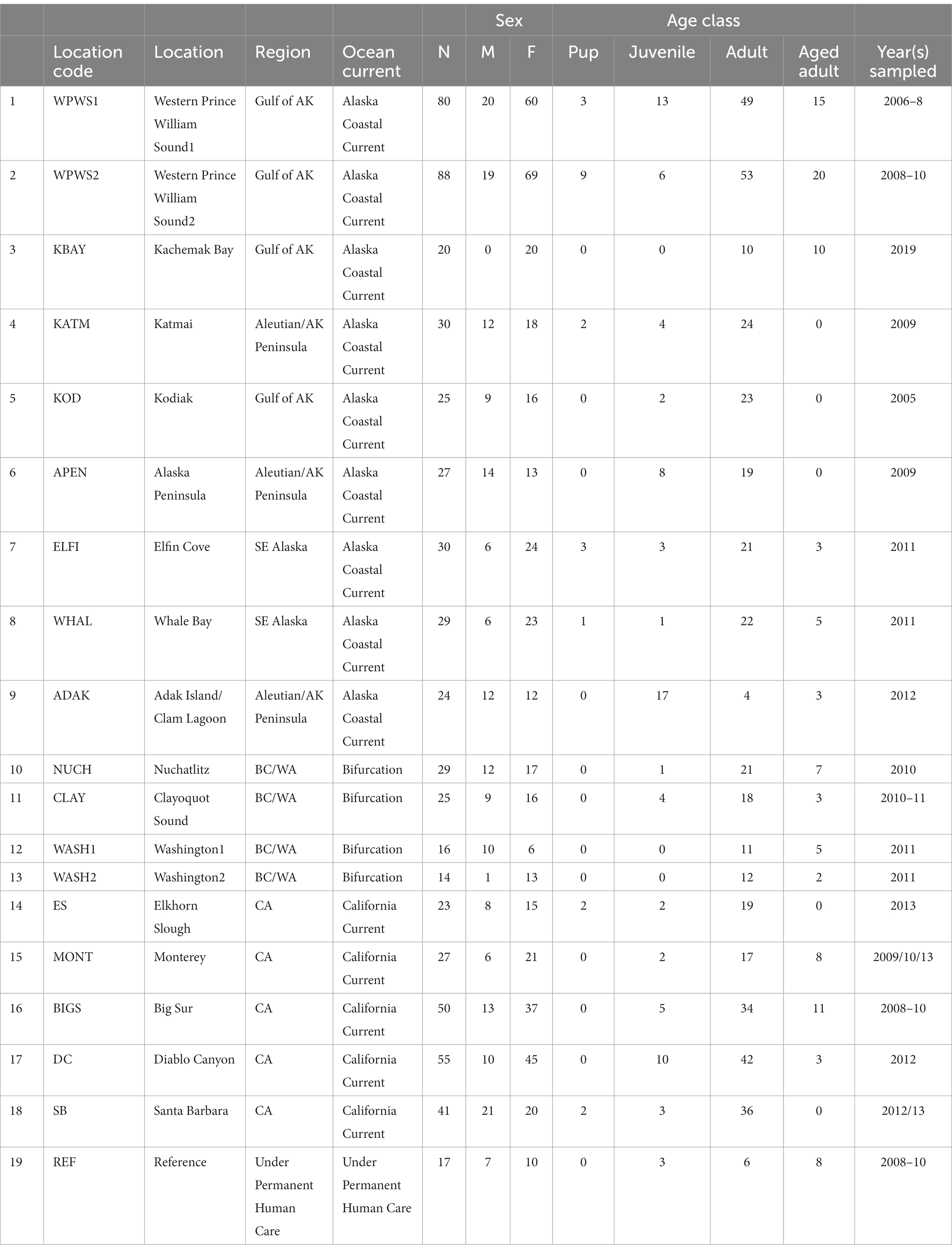
Table 1. Population locations, number of samples, sex, age class, and sampling year.
2. Materials and methods
2.1. Study area
The 19 sea otter populations we have chosen to include in this study are located from near Santa Barbara, California, north to Prince William Sound (WPWS), Alaska and west to Adak, Alaska (ADAK) (Figure 1; Table 1). Our “reference” (REF) group of sea otters were under permanent human care and were sampled from aquaria within the United States and Canada (Bowen et al., 2012). Each reference sea otter was classified as “clinically normal” by associated veterinarians. Although stress is inherent in life under permanent human care for wildlife species, environmental stressors are thought to be minimized in an aquarium setting. Additionally, gene expression levels in reference sea otters were not statistically different from gene expression levels in free-ranging sea otters inhabiting an area with minimal environmental stressors (Alaska Peninsula) (Bowen et al., 2016). In CA, the current range of the sea otter extends from near Los Angeles in the south to near San Francisco in the north, areas of relatively high human impacts. However, the range includes some coastline along the Big Sur coast, in Central CA, where human densities are low, and the watersheds are protected to some extent by governmental resource agencies. The sea otter populations occurring in Washington state (WASH1 & 2), British Columbia (CLAY, NUCH), and Southeast Alaska (ELFI, WHAL) resulted from reintroductions in the 1960’s and 1970’s to restore the species (Jameson et al., 1982). Sea otters in south-central and south-west Alaska (WPWS1 & 2, KBAY, KATM, KOD, APEN, ADAK) are the descendants of remnant populations that survived near those locations. Human densities along the north Pacific coastline generally decline from south to north, and given the areas in which our study animals were sampled, we expect that human degradation of watersheds likely diminish along this gradient. Within each distinct sea otter population, the full range of nearshore habitats are occupied, including sandy shorelines, protected soft sediment bays and estuaries, and exposed rocky shorelines.
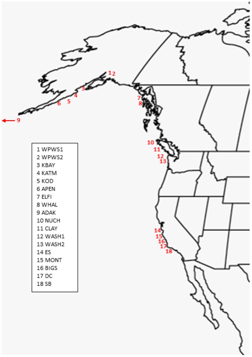
Figure 1. Population locations of sea otters included in the analysis. Locations numbered from North to South (Table 1). Captive otters (N = 17) not shown (see Bowen et al., 2012 for details).
Sea otters were captured using Wilson traps (Wendell et al., 1996) or tangle nets and brought immediately to a shipboard or shore station for processing. All sea otters were anesthetized with fentanyl citrate and midazolam hydrochloride (Monson et al., 2001; Murray, 2015) prior to processing. Nearly all the animals (exception AK Pen) were captured with the Wilson trap that targeted resting groups of animals without knowledge of age or sex. At the Alaska Peninsula site, sea otters were captured using tangle nets that targeted active animals, also without regard to age or sex. Because the true age and sex composition could not be determined for each population, we were unable to evaluate the composition of the sampled population relative to the entire population. However, as the capture methods were not known to be biased toward age or sex, we concluded that the captured individuals were representative of the population being sampled.
2.2. Blood collection and RNA extraction
A 2.5 ml sample from each sea otter was drawn directly into a PAXgene blood RNA collection tube (PreAnalytiX, Zurich, Switzerland) from either the jugular or popliteal veins and then frozen at −80°C until extraction of RNA (Bowen et al., 2012). The RNA from blood in PAXgene tubes was isolated according to manufacturer’s standard protocols, which included an on-column DNase treatment to remove contaminating gDNA (silica-based microspin technology), and the extracted RNA stored at −80°C until analysis. We measured the concentration and clarity on a Qubit 3.0 Fluorometer using the RNA, DNA and RNA IQ Assay Kits (Life Technologies, Carlsbad, CA, USA).
2.3. cDNA synthesis
A standard cDNA synthesis was performed on 2 ug of RNA template from each animal. Reaction conditions included 4 units reverse transcriptase (Omniscript®, Qiagen, Valencia, CA), 1 μM random hexamers, 0.5 mM each dNTP, and 10 units RNase inhibitor, in RT buffer (Qiagen, Valencia, CA). Reactions were incubated for 60 min at 37°C, followed by an enzyme inactivation step of 5 min at 93°C, and then stored at −20°C until further analysis.
2.4. Real-time PCR
The 13 genes chosen for the expression profile analysis represent multiple physiological systems that play roles in immuno-modulation, inflammation, cell protection, tumor suppression, cellular stress-response, xenobiotic metabolizing enzymes and antioxidant enzymes (Table 2). These genes can be modified by biological, physical, or anthropogenic impacts and consequently can provide information on the general type of stressors present in a given environment.
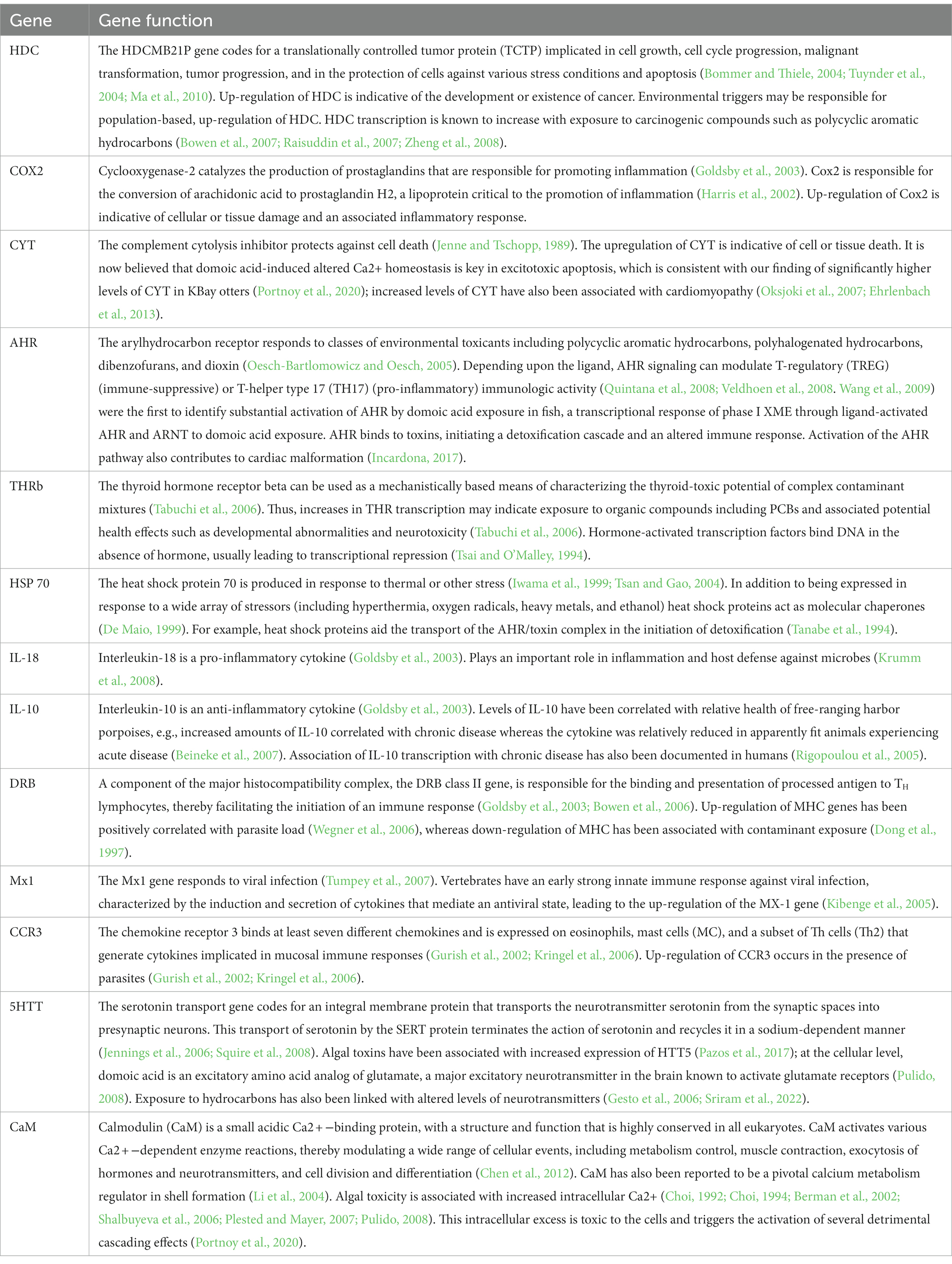
Table 2. Thirteen genes selected for sea otter-specific qPCR analytical panel and their functions.
Real-time PCR systems for the individual, sea otter-specific reference or housekeeping gene (S9) and genes of interest were run in separate wells (see Supplementary Table S1 for primer sequences). Briefly, 1 μL of cDNA was added to a mix containing 12.5 μL of Quanti-Tect SYBR Green Master Mix [5 mM Mg2+] (Qiagen, Valencia, CA), 0.5 μL each of forward and reverse sequence specific primers, and 10.0 μL of RNase-free water; total reaction mixture was 25 μL. The reaction mixture cDNA samples for each gene of interest and the S9 gene were loaded into 96 well plates in duplicate and sealed with optical sealing tape (Applied Biosystems, Foster City, CA). Reaction mixtures containing water, but no cDNA, were used as negative controls; thus approximately 3–4 individual sea otter samples were run per plate.
Amplifications were conducted on a Step-One Plus Real-time Thermal Cycler (Applied Biosystems, Foster City, CA). Reaction conditions were as follows: 50°C for 2 min, 95°C for 15 min, 40 cycles of 94°C for 30 s, 60°C for 30 s, 72°C for 31 s, and an extended elongation phase at 72°C for 10 min. Reaction specificity was monitored by melting curve analysis using a final data acquisition phase of 60 cycles of 65°C for 30 s and verified by direct sequencing of randomly selected amplicons. Cycle threshold crossing values (CT) for each of the genes of interest were normalized to the S9 housekeeping gene.
2.5. Statistical analysis
We used statistical methods with different approaches to examine the interpretive outcomes of different statistical perspectives and how these influence our assessment of “health.” Traditionally, gene expression data are presented as CT (Threshold crossing) values. According to the ΔCT method (Livak and Schmittgen, 2001), we normalized values (internal reference gene CT subtracted from the gene of interest CT). Often, ΔΔCT (Livak and Schmittgen, 2001) is used; in that case the normalized value of the target gene is compared with the CT of a calibrator sample (reference population). In some instances, ΔΔCT values are then transformed. Real-time PCR data are represented as normalized CT values; the lower the CT, the higher the quantity of transcripts. We used generalized linear multivariate models (GLMV) to visually describe gene transcript profiles by location (Figure 2) [Note: KOD was included in the GLMV analysis but not in further analyses, because at the time of sampling and analysis for KOD, three genes were yet to be included in the expression panel (CCR3, HTT5, CaM)].We then evaluated the association between gene transcription levels and location with redundancy analysis (RDA) (Figure 3; Legendre and Legendre, 2012). Redundancy analysis allows the analysis of multiple response variables (in this case the 13 genes in our transcript panel) by combining multiple regression and principal components analysis (PCA). Two types of ordination scores are derived in an RDA (Legendre and Legendre, 2012): (1) those quantifying relationships between response and predictor variables (linear combinations of predictor variables, i.e., the multiple regression component); and (2) those that quantify the associations between response variables and sampling units (weighted sampling unit scores, i.e., the PCA component). Our sampling units comprised 625 sea otters separated into 18 groups based on location (Table 1). We evaluated significance of the overall ordination with Monte Carlo tests (N = 999; Legendre and Legendre, 2012). We conditioned the Monte Carlo simulations on location, which we specified as a random effect in the RDA.
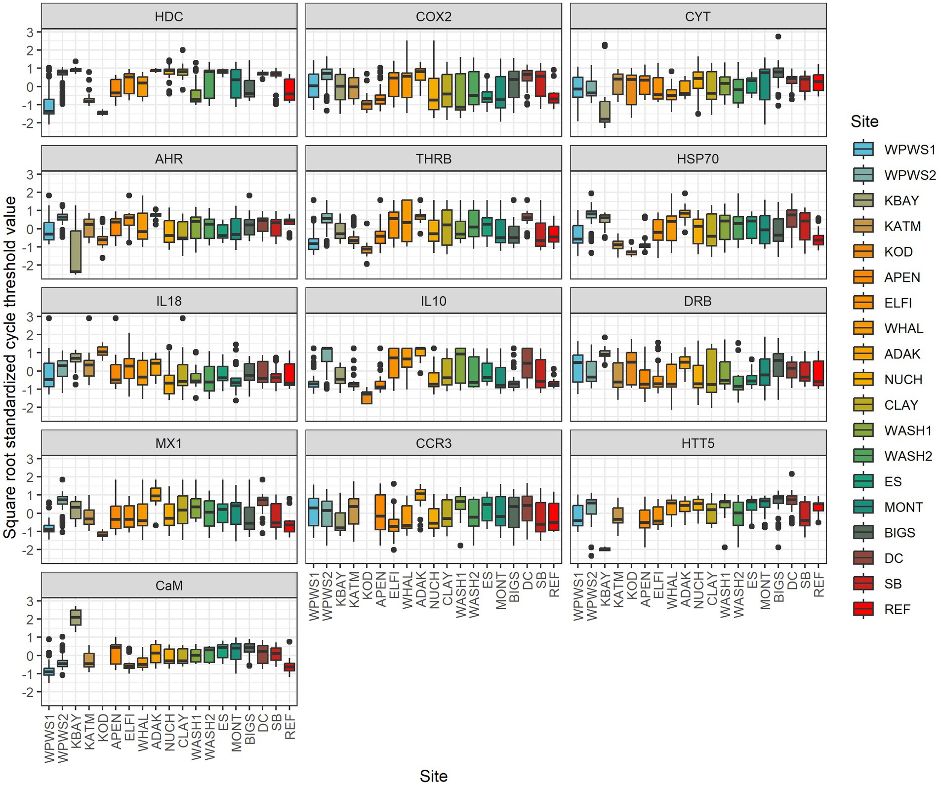
Figure 2. Generalized linear multivariate models (GLMV) were used to visually describe gene transcript profiles by location. Distribution of mean cycle threshold (CT) values and confidence intervals across genes targeted by the panel of 13 primer pairs for 19 populations. Note: KOD is missing data for CCR3, HTT5, and CaM. Real-time PCR data are represented as normalized values (NVs); the lower the NV, the higher the quantity of transcripts. All values were pre-standardized to mean 0 and sd 1 in order to visualize inter-site variation on common scale. Data was then transformed based on the square root standardized CT values (Negative values are transformed by taking the sqrt of the absolute value and reattaching the negative sign). This transformation reduces the kurtosis (heavy tails) above and below the 0 and enables outliers to be included in the graph without flattening the variation patterns in the midsection of the graph. Sites have one of 3 general patterns: (1) otters distributed widely above and below average gene expression (boxes that encompass 0), (2) otters generally expressing more than average (boxes below 0), and (3) otters that are generally under-expressing (boxes above 0).
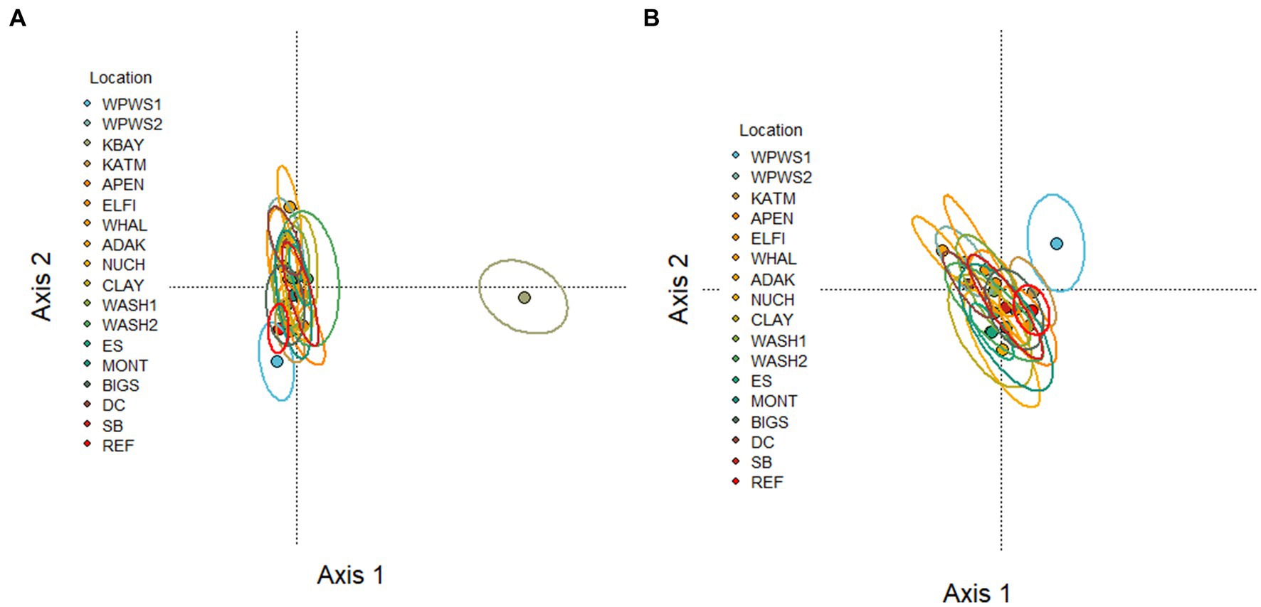
Figure 3. (A,B) RDA Redundancy analysis of the occurrence of 13 genes in 18 populations of sea otters (small circles) captured between 2006 and 2019. Large circles indicate population centroids. KOD sites omitted due to lack of CCR3, HTT5, and CaM (KOD samples were analyzed prior to development of CCR3, HTT5, and CaM assays). (A) The differences between KBAY and other sites are dominating the variation in this figure, making it difficult to pick out the differences among the other locations. (B) The same analysis is repeated with KBAY omitted. Figures with individual otters plotted are shown in Supplementary Figure 1.
Subsequent to RDA, and in order to illustrate within population differences, we used gene profiling based on per gene and per otter response correlation for the Kachemak Bay (KBAY) otters, using normalized qPCR data obtained from each individual otter, which were subjected to hierarchical clustering using Genesis software (Genesis, Graz, Switzerland). Average dot product metric, with complete linkage clustering, was used to generate a heatmap profile of gene expression (Figure 4; Connon et al., 2012).
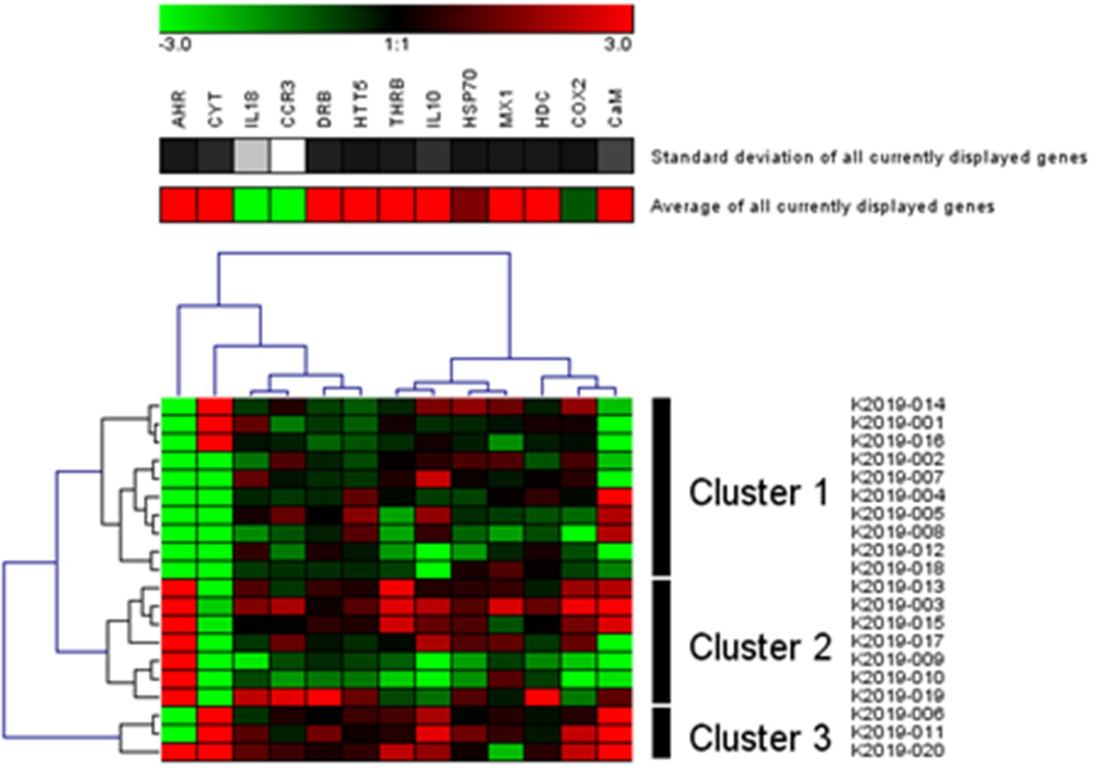
Figure 4. Gene profiling: Transcription matrix of 13 target genes in sea otters captured in 2019 in Kachemak Bay, AK (Hierarchical clustering with complete linkage disequilibrium; Genesis, Graz, Switzerland). Green indicates higher relative transcription levels and red indicates lower relative transcription levels.
We used a generalized linear latent variable analysis (GLLVA), a key approach for modeling multivariate abundance data, to identify associations between population/location and transcript level (Figure 5; Skrondal and Rabe-Hesketh, 2004). The generalized linear latent variable model (GLLVM) extends the basic generalized linear model to multivariate data using a factor analytic approach, incorporating a small number of latent variables (interpreted as ordination axes) for each site accompanied by factor loadings to model correlations between responses (Niku et al., 2019).
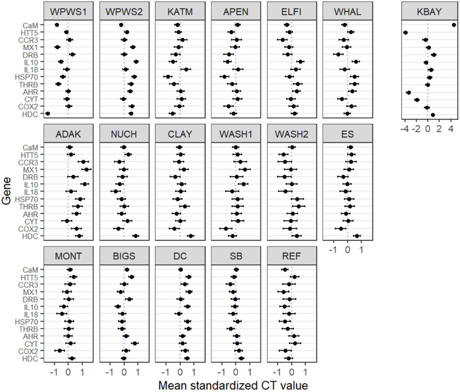
Figure 5. Generalized linear latent variable analysis (GLLVA). Plots of the point estimates (ticks) for coefficients of the genes and their 95% confidence intervals (lines) for the GLLVM. X axes represent transcription level estimates (deviations from the mean) after accounting for within and across population deviations. The vertical 0 reference line the mean transcription level across all populations. Y axes represent genes of interest. Many of the 95% confidence intervals do not include zero, indicating that many of the genes exhibit evidence of a strong association between population/location and transcript level. The KBAY population is plotted separately on the right on a different scale due to wider variations compared to the other populations.
We evaluated homogeneity of the variance–covariance matrices among the groups with a distance-based test (beta dispersion test; Anderson et al., 2006; Figure 6).
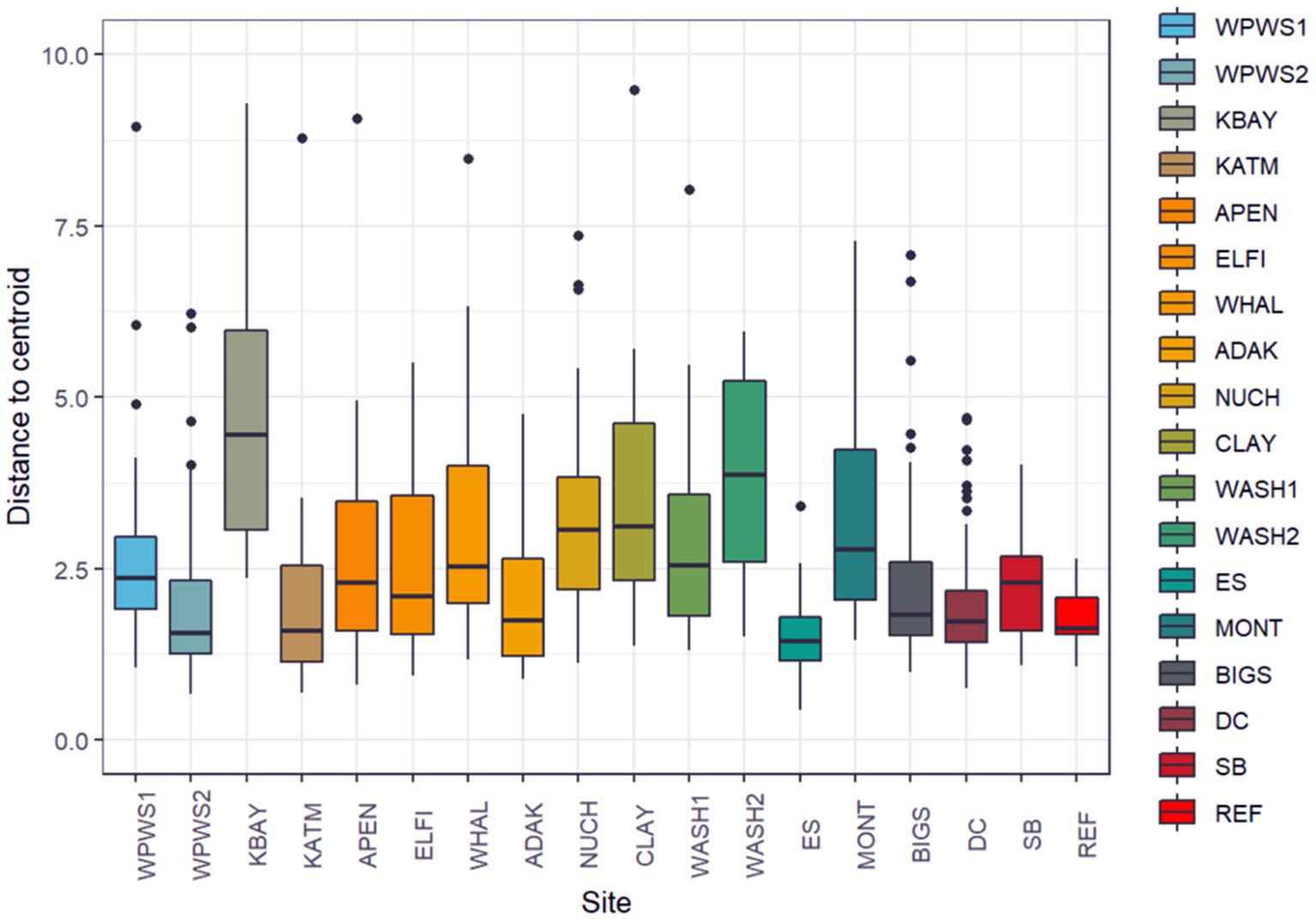
Figure 6. We evaluated homogeneity of the variance–covariance matrices among the groups with a distance-based test (beta dispersion test; Anderson et al., 2006). Population groups are sorted from North to South geographically. The null hypothesis was rejected with distance to centroid beta dispersion p < 1.106e−12.
All analyses (except the heatmap analysis, Genesis, Graz, Switzerland, Figure 4) were conducted in Program R (R Development Core Team, 2012). We used the vegan package for the RDA and beta dispersion test.
3. Results
Using a generalized linear multivariate model (GLMV) to visually describe gene transcript profiles by gene and population (Table 3), Figure 2 illustrates the distribution of mean cycle threshold (CT) values and confidence intervals across genes targeted by the panel of 13 primer pairs for 19 populations. Although most population responses were overlapping to some degree, clear differences exist among responses for genes and populations (Figure 2; Table 3). The most striking differences occurred for (1) HDC, for which Western Prince William Sound 1 (WPWS1) had significantly higher expression than WPWS2 and any of the other populations, (2) CYT, for which Big Sur (BIGS) had significantly lower expression than any of the other populations, and CaM which had lower levels of expression in KBAY than in any other population.
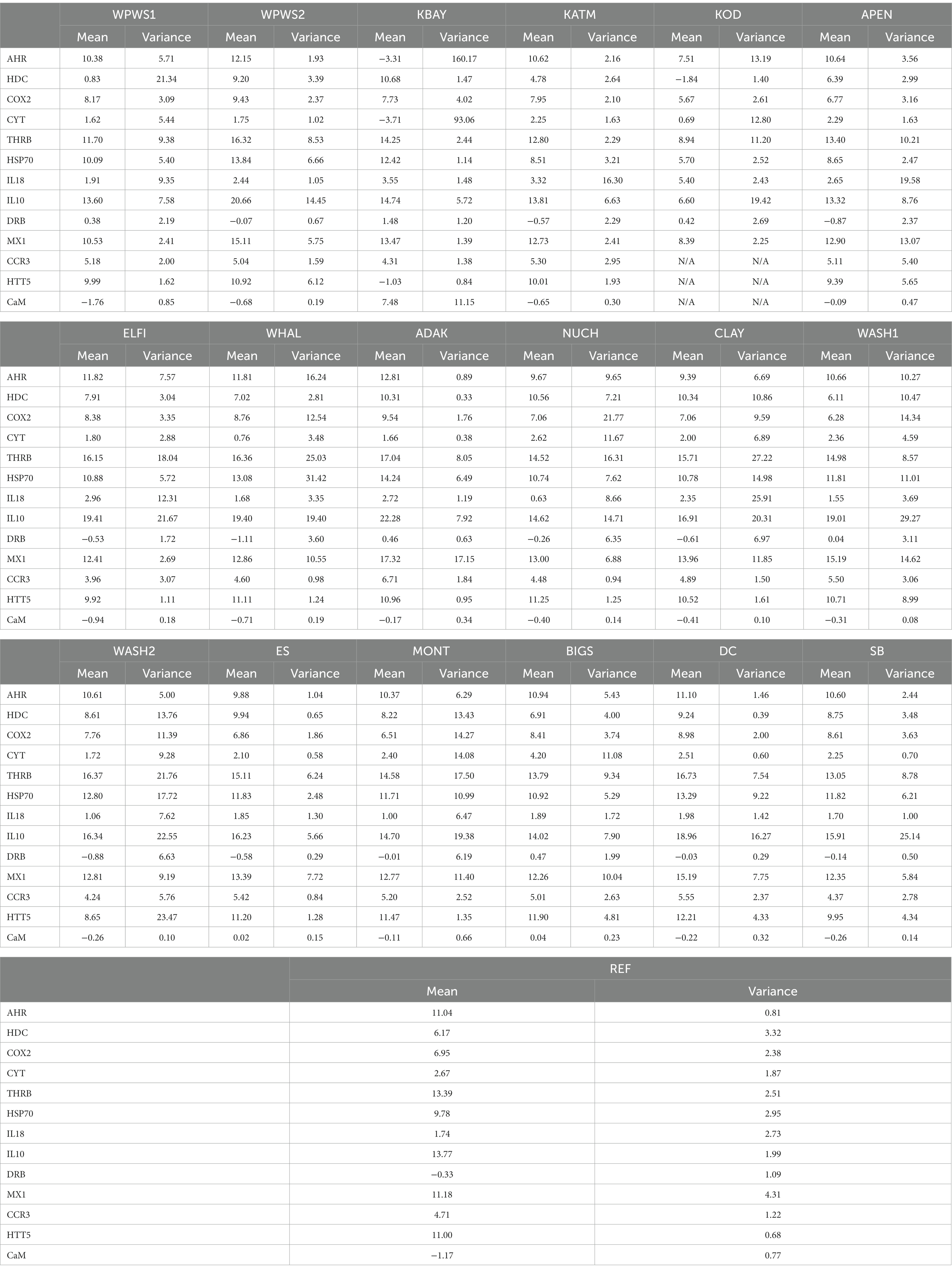
Table 3. Means and variances for all populations.
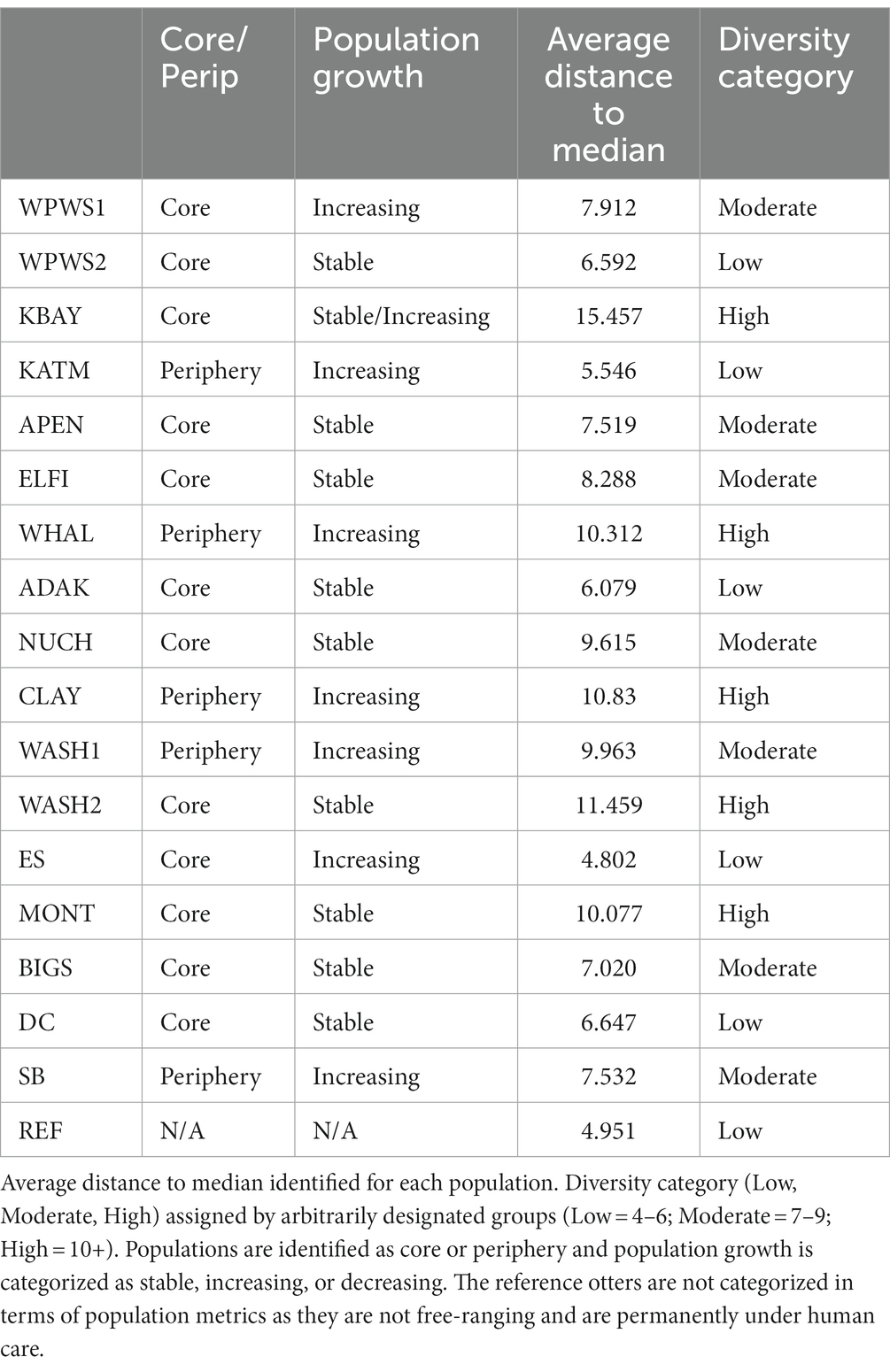
Table 4. Beta diversity by population.
The RDA of the occurrence of 13 genes in 18 populations of sea otters captured between 2006 and 2019 is depicted in Figures 3A,B. The variation in Figure 3A is dominated by the differences between KBAY and other locations. The same analysis was repeated (Figure 3B) with KBAY omitted, showing WPWS1 as the most transcriptionally divergent population. In the RDA, location explained 32% of the total variation in transcription levels; 87% of this can be explained by the first three axes (accumulated constrained eigenvalues); 68% of the variation is under the influence of variables that were not included in the model or measured. Hierarchical cluster analysis and subsequent heat map generation were conducted using individual sea otter transcription data (Figure 4). Heat map analysis was successful in demonstrating structuring of the KBAY population based on transcriptional differences. Cluster 1 was defined predominately by relatively high levels of AHR and CYT expression as well as by elevated CaM in 7 out of 10 otters. Cluster 2 was defined by relatively lower levels of AHR expression, high CYT expression and mixed CaM. Cluster 3 was identified by mixed AHR and relatively low CYT and CaM expression.
The GLLVA identified many 95% confidence intervals that do not include zero, indicating that many of the genes exhibit evidence of a strong association between population/location and transcript level (Figure 5). The GLLVA identifies strong associations between population and transcript levels for at least one gene in each population: WPWS1 (7), WPWS2 (7), KATM (4), APEN (4), ELFI (4), WHAL (4), KATM (6), ADAK (8), NUCH (2), CLAY (1), WASH1 (3), WASH2 (1), ES (2), MONT (1), BIGS (4), DC (7), SB (3), and REF (3).
We evaluated homogeneity of the variance–covariance matrices among the groups with a distance-based test (beta dispersion test; Figure 6; Table 4; Anderson et al., 2006). For each wild population, abundance was estimated more than once (often annually) prior to sampling, allowing the classification of each population as either stable, declining, or increasing. Populations were assigned the status of “core” or “periphery” (Table 4); core indicates “long established” (10–20 years minimum), while periphery indicates relatively newly established (<10 years). Population groups are sorted from North to South (latitudes) geographically. The null hypothesis, no differences among populations, was rejected with distance to centroid beta dispersion p < 0.001.
4. Discussion
This study reveals some of the challenges and possible uses of gene expression data for describing wildlife health and brings into question choices of study design, methods of statistical analysis, and interpretation. For example, using distribution of mean cycle threshold (CT) values and confidence intervals for individual genes of interest to describe population differences leads to complicated conclusions about population health and resilience (Figures 2, 5). Before we can interpret this data, we should determine whether it is “good” or “bad” for a gene to be up- or down-regulated. If a gene has relatively high(er) levels of expression, is that necessarily a negative indication? Higher levels of expression indicate a response to something, perhaps a stressor, but if it’s an appropriate response resulting in mitigation of a stressor, that should have a positive outcome for the individual or population. For example, in Figure 5, there are four predominant patterns: (1) populations distributed above and below average gene expression (boxes that encompass 0), (2) populations generally expressing more than average (boxes below 0), (3) populations that are generally under-expressing (boxes above 0), and (4) populations whose values are generally very close to the mean, with little variation across the 13 genes. Moderate (i.e., close to the average) levels of gene expression may be indicative of ecosystem or population equilibrium; while very low levels of gene expression could indicate either a lack of stressors, or potentially an inability to mount a molecular response, perhaps due to a lack of biological resources. Additional data on individuals or the population would be needed to clarify and support interpretation of the gene expression results (Vera-Massieu et al., 2015; Weiße et al., 2015; Strandin et al., 2018).
Although similar in output, GLMV (Figure 2) and GLLVA (Figure 5) use slightly different approaches to identify gene contributions to the separation of populations in statistical space. In fact, GLMV depicts raw data and is thus purely descriptive, identifying general patterns. Conversely, GLLVA is model based and identifies statistical significance, allowing for interpretations and conclusions. However, the outcome of the two analyses lead to similar interpretations. For example, we can say with certainty that WPWS1 has by far the highest level of HDC expression of the groups in our study. The HDC gene codes for a translationally controlled tumor protein (TCTP) implicated in cell growth, cell cycle progression, malignant transformation, tumor progression, and in the protection of cells against various stress conditions and apoptosis (Bommer and Thiele, 2004; Tuynder et al., 2004; Ma et al., 2010; Table 1). HDC transcription is known to increase with exposure to carcinogenic compounds such as polycyclic aromatic hydrocarbons (PAH; Bowen et al., 2007; Raisuddin et al., 2007; Zheng et al., 2008). We can hypothesize that HDC might be responding to lingering oil from the Exxon Valdez oil spill (EVOS) in 1989 (Bodkin et al., 2012), which is consistent with WPWS sea otters having continued EVOS-related survival effects lasting until ~2010 (Monson et al., 2001; Ballachey et al., 2014). Again, although an appropriate response can be interpreted as a “good” thing, there are associated costs. Molecular activity is physiologically costly (Vera-Massieu et al., 2015; Weiße et al., 2015; Strandin et al., 2018). Perhaps the largest cost is the reallocation of nutrients and energy from one portion of an individual’s resource budget to other metabolic functions. Mitigation of stressors imposes demands on animals above those normally required to sustain life and may result in reduction of fitness evidenced by decreased reproductive capability, increased susceptibility to disease, or disadvantageous behavioral changes (Martin et al., 2010; Graham et al., 2011).
Other differences in distribution of mean cycle threshold (CT) values and confidence intervals of note include relatively low levels of CYT in the BIGS population and the relatively low levels of eight of the 13 genes in the WPWS2 population. CYT, the complement cytolysis inhibitor, protects against or inhibits cell death (Jenne and Tschopp, 1989). Relatively low levels of CYT expression might be indicative of an inability to or lack of a need to kill pathogens. Again, population level context would help with interpretation. The low expression levels seen in WPWS2 sea otters could be consistent with an inability to mount effective responses to pathogens, contaminants, injury, or other stressors when compared to other groups. In fact, disease and mortality do not necessarily indicate a disease-induced population decline, because the elevated frequency of disease is a common manifestation of resource limitation in many wildlife species, which in turn is influenced by prey availability and environmental conditions (Post et al., 2013; Wobeser, 2013). For example, WPWS2 may no longer have mortality level stressors related to PAHs but may continue to have non-lethal, yet disadvantageous, levels of stressors still related to oil spill effects. Infectious diseases occur in all ecosystems, both healthy and unhealthy, and play an important role in structuring biological communities (Tracy et al., 2019). A determination of WPWS2 at or exceeding carrying capacity and thus likely nutrient limited would help support the theory of resource limitation. Energy intake rates have been shown to be a useful indicator of resource availability in sea otters (Dean et al., 2002; Coletti et al., 2016). Estimated energy intake rates for sea otters living in WPWS averaged ~6.5 kcal/min between 2010 and 2012 (Coletti and Wilson, 2015), which is consistent with a population near carrying capacity and supports the theory of resource limitation.
Previous work by Bowen et al. (2022), identified abnormally high levels of AHR and CYT as well as low levels of CaM in KBAY otters; these differences are also identified in our current analyses. Brief interpretation indicates possible exposure to an algal toxin; the KBay sea otters had transcript profiles very different from those of otters with suspected oil exposure (WPWS1), and in fact, oil exposure is not suspected to be a factor influencing transcript profiles in KBay (Bowen et al., 2022). At the time of sampling in 2019, the KBAY population was stable or increasing (Table 1). Intuitively, this may conflict with the extremely divergent gene expression patterns identified in KBAY otters. We can surmise that the KBAY otters were responding to a stressor, and, at least in the short-term, providing some level of mitigation of that stressor. However, we do not know the longer-term consequences of this exposure. Even without near-term morbidity or mortality, will exposure to this particular stressor affect population health in the long-term?
KBAY was also remarkable from the analysis of population centroids in the RDA (Figure 3), in which it was separated from all other groups along axis 1. As stated above, we identified a very high level of CYT, AHR, and HTT5, and low level of CaM expression in KBAY in relation to the other groups. Little discernable separation occurred along axis 2 in the RDA and population centroids were obscured. In general, there are still unmeasured factors influencing the gene expression levels, however, the environmental variables have a very strong influence. What about within population variation? For example, the gene expression KBAY profile appears to split into two groups. Although we found no statistical link among age, sex, or capture location, and gene expression profile within this population, further examination revealed stark differences in gene expression levels within the KBAY otter population (Figure 4). The KBAY population may have been exposed to one or more harmful algal toxins (Bowen et al., 2022). Harmful algal blooms may not be uniformly distributed, and prey items may concentrate or bioaccumulate toxins differently. As well, dietary specialization is a well-known attribute of the sea otter; the diet of sea otters in KBAY is diverse, including clams and mussels that may sequester biotoxins and crustaceans that may not (Tinker et al., 2008). Therefore, we could predict that this within-population split has to do with foraging location or prey preferences.
Due to the degree KBAY drove placement of the other otter populations in RDA space, we repeated the analysis without KBAY otters (Figure 3B). When KBAY is removed, the remaining otter populations spread out somewhat in RDA space, The most notable separation in this case is WPWS1, which separated from all other groups along axis 1 and 2 (Figure 3B). We identified very high levels of HDC expression in WPWS1 in relation to the other groups (Figure 2). As described in Miles et al. (2012), expression profiles of WPWS1 otters in comparison with clinically normal reference otters indicated exposure to lingering oil.
Historically, the term beta diversity has been used in an ecological context to represent the difference in species composition between local and regional assemblages (de Juan et al., 2013). Thus, diversity has been suggested as a measure of ecosystem resilience (de Juan et al., 2013); greater variation in beta diversity could be an early warning sign of declining host health (Fackelmann and Sommer, 2019). However, considering the current and rapidly increasing nearshore marine ecosystem degradation due to cumulative stressors associated largely with climate change, there is an urgent need to identify variables that might indicate changes in ecosystem state (de Juan et al., 2013). Although beta diversity is a promising measure of ecosystem resilience in the context of species richness, can we apply this to levels of gene expression? Our beta dispersion test identified significantly different levels of variation in quantities of gene expression across populations (Figure 6). Additionally, the captive population had the smallest amount of diversity in terms of gene expression, which might indicate more stable environments with fewer stressors.
Research in unicellular organisms has linked noise (heterogeneity/variation) in gene expression to population growth rate (Keren et al., 2015). We have not found studies that used levels of beta dispersion in gene expression as a measure of population or ecosystem health or resilience. However, extrapolation from the unicellular model to the population level may be possible. For example, variability in expression in unicellular organisms is anti-correlated to population average gene expression, which in turn is tightly coupled to growth rate (Tyson et al., 1979; Ingraham et al., 1983; Bar-Even et al., 2006; Newman et al., 2006; Brauer et al., 2008; Klumpp et al., 2009; Taniguchi et al., 2010; Keren et al., 2013, 2015). This brings us to two distinct approaches of quantifying variation in gene expression, intrinsic vs. extrinsic variability. Intrinsic variability describes the variation at the level of a single gene due to the stochastic nature of the transcriptional process, while extrinsic variability relates to the variability across different genes as a result of population dynamics and environment (Keren et al.’s, 2015). As far as we know these concepts have not yet been applied to gene expression studies in wildlife; accurate interpretation will require further exploration.
In terms of growth, work to date has focused on growth of a cell, not a population. However, the concept therein may be applied (with modifications) to wildlife populations. For example, in Keren et al. (2015) study of gene expression in yeast, harsher environmental conditions were found to reduce growth rates. At least conceptually, this also applies to wildlife populations; greater environmental pressures require greater levels of mitigation, evidenced by greater levels of variation in gene expression. Gene expression mitigation uses resources normally reserved for maintenance of growth and reproduction. An ensuing resource allocation imbalance occurs, ultimately resulting in slower growth rates, either at the cellular or population level (Martin et al., 2010; Graham et al., 2011). However, this may not be immediately evident. For example, otters in the KBAY population demonstrate the highest amount of variation in our study, and yet as of 2019 the KBAY population was stable (Esslinger et al., 2021); what we do not know are the long-term effects of the particular stressor and the resulting molecular mitigation strategies. How do we interpret the relatively little variation demonstrated by several populations (see Figure 6)? From what we know, we can speculate that the low variation in the WPWS2 and ADAK populations is because those populations are nutritionally limited, making increased expression difficult if not impossible. Just recently, the KATM population was determined to be food-limited but is an area with little or no known remarkable environmental stressors (Coletti et al., 2016; Tinker et al., 2021). The ES population may exhibit low variability because of its small size and homogenous landscape. The REF population includes only animals under permanent human care. As such, their environment is tightly regulated with little variation in extrinsic stimuli, which can result in limited variability. Moderate variability (WPWS1, APEN, ELFI, NUCH, WASH1, BIGS, SB) includes populations clearly responding to stressors as well as populations thought to be at equilibrium. Aside from KBAY, populations categorized as having highly variable gene expression (KBAY, WHAL, CLAY, WASH2, MONT) showed significant differences in gene expression from other populations. Note that three or four of these five populations may be periphery populations, which may account for the high variation. However, in this exercise, we examined variability across a gene panel. For a more complete picture and more refined interpretation as it relates to individual and population health, we should consider variation on a per gene basis. We should also consider formally collecting (if needed) and incorporating (when available) other measurements at both the ecosystem level and individual level that may aid in interpretation (such as prey availability and body condition). Level of variation might also reflect where the population is heading, rather than where it has been. It is important to recognize that our determination of population status based on length of occupation and surveys of abundance are by design, hindcasting, in terms of what the population has been doing, not where the next data point might lie on that trend.
In our study, interpretations based on variances and means overlapped to some degree. For example, those populations in the low diversity category all had suppressed or low levels of gene expression, representing limited nutritional resources or limited extrinsic stressors, respectively. These two states are quite different, and interpretation of results requires additional knowledge of the system as a whole. In contrast, populations in the moderate and high diversity categories (with the exception of KBAY) did not align with analyses focused on mean expression levels. Clearly there are interpretations and inferences we are not yet making based on these findings.
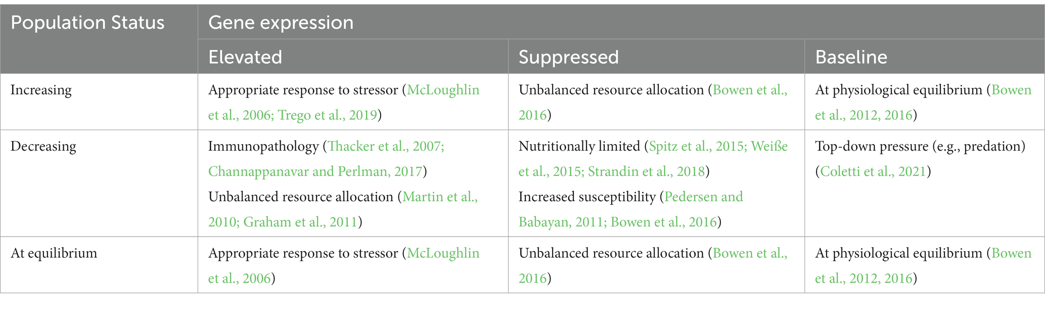
Table 5. Using gene expression to conceptualize wildlife population status as a measure of health.
5. Implications
Determination of population “health” will require several choices and definitions (including of health itself): perspective (including choice of sentinel species, population inclusions, time frame, etc.), measurement techniques (molecular to population level), and statistical analysis choices (focus on population means or population variation). Ultimately, determination of population or ecosystem health will require information from many disciplines, contextualized to specific scenarios and goals. Inclusion of fine scale, mechanistic tools such as gene expression are necessary to begin to understand why populations are healthy or not, and to formulate strategies for recovery. Without these, we are left with only a simple and partial answer regarding population status. At some point, which we have not quite reached on a global scale, gene expression may be linked to wildlife population status as measure of health. A conceptualized example of the relationship between variation in gene expression and population status is provided in Table 5.
This brings us back to one of our original questions: is divergent gene expression good or bad? Similarly, is divergent variation in gene expression good or bad? Both appear to be context dependent, and neither can be answered without first defining the optimum or healthy system. Long-term monitoring programs could be leveraged to address data gaps and provide consistent ecosystem level-inputs of a variety of metrics, which would allow for interpretation of these results more fully.
Data availability statement
The raw data supporting the conclusions of this article will be made available by the authors, without undue reservation.
Ethics statement
Field activities were conducted under the Marine Mammal Protection Act USFWS permit (MA041309). No animals were used in the current study. Animal care and permit information can be found in the cited literature.
Author contributions
LB, JY, AM, and JB contributed to conception and design of the study. SW organized the database. JY and LB performed the statistical analyses. LB wrote the first draft of the manuscript. DM, BB, HC, JY, MM, and JB wrote sections of the manuscript. All authors contributed to the article and approved the submitted version.
Funding
USGS Ecosystems Mission Area provided funding for original field study, data analyses, interpretation, and writing.
Acknowledgments
The authors would like to thank Rob Klinger for his invaluable assistance as a statistical sounding board. They greatly appreciate the hard work of all who participated in gathering samples and data for this project; you are far too many to list here, but this research would not have been possible without you. Any use of trade, firm, or product names is for descriptive purposes only and does not imply endorsement by the U.S. Government.
Conflict of interest
The authors declare that the research was conducted in the absence of any commercial or financial relationships that could be construed as a potential conflict of interest.
Publisher’s note
All claims expressed in this article are solely those of the authors and do not necessarily represent those of their affiliated organizations, or those of the publisher, the editors and the reviewers. Any product that may be evaluated in this article, or claim that may be made by its manufacturer, is not guaranteed or endorsed by the publisher.
Supplementary material
The Supplementary material for this article can be found online at: https://www.frontiersin.org/articles/10.3389/fevo.2023.1157700/full#supplementary-material
References
Álvarez-Muñoz, D., Llorca, M., Blasco, J., and Barceló, D. (2016). “Chapter 1–Contaminants in the marine environment” in Marine ecotoxicology. eds. J. Blasco, P. M. Chapman, O. Campana, and M. Hampel (Cambridge, MA: Academic Press), 1–34.
Anderson, M. J., Ellingsen, K. E., and McArdle, B. H. (2006). Multivariate dispersion as a measure of beta diversity. Ecol. Lett. 9, 683–693. doi: 10.1111/j.1461-0248.2006.00926.x
Androulakis, I. P., Yang, E., and Almon, R. R. (2007). Analysis of time-series gene expression data: methods, challenges, and opportunities. Annu. Rev. Biomed. Eng. 9, 205–228. doi: 10.1146/annurev.bioeng.9.060906.151904
Ballachey, B. E., Bodkin, J. L., Esler, D., and Rice, S. D. (2014). “Lessons from the 1989 Exxon Valdez oil spill: a biological perspective” in Impacts of oil spill disasters on marine habitats and fisheries in North America (Milton Park: Taylor & Francis), 181.
Bar-Even, A., Paulsson, J., Maheshri, N., Carmi, M., O’Shea, E., Pilpel, Y., et al. (2006). Noise in protein expression scales with natural protein abundance. Nat. Genet. 38, 636–643. doi: 10.1038/ng1807
Beineke, A., Siebert, U., Muller, G., and Baumgartner, W. (2007). Increased blood interleukin-10 mRNA levels in diseased free-ranging harbor porpoises (Phocoena phocoena). Vet. Immunol. Immunopathol. 115, 100–106. doi: 10.1016/j.vetimm.2006.09.006
Berman, F. W., LePage, K. T., and Murray, T. F. (2002). Domoic acid neurotoxicity in cultured cerebellar granule neurons is controlled preferentially by the NMDA receptor Ca2+ influx pathway. Brain Res. 924, 20–29. doi: 10.1016/s0006-8993(01)03221-8
Blanchong, J. A., Robinson, S. J., Samuel, M. D., and Foster, J. T. (2016). Application of genetics and genomics to wildlife epidemiology. J. Wildl. Manag. 80, 593–608. doi: 10.1002/jwmg.1064
Bodkin, J. L., Ballachey, B. E., Coletti, H. A., Esslinger, G. G., Kloecker, K. A., Rice, S. D., et al. (2012). Long-term effects of the ‘Exxon Valdez’oil spill: sea otter foraging in the intertidal as a pathway of exposure to lingering oil. Marine Ecol. Prog. Ser. 447, 273–287. doi: 10.1073/pnas.120163397
Bommer, U. A., and Thiele, B. J. (2004). The translationally controlled tumour protein (TCTP). Int. J. Biochem. Cell Biol. 36, 379–385. doi: 10.1007/978-3-319-67591-6_4
Bowen, L., Aldridge, B. M., Miles, A. K., and Stott, J. L. (2006). Expressed MHC class II genes in sea otters (Enhydra lutris) from geographically disparate populations. Tissue Antigens 67, 402–408. doi: 10.1111/j.1399-0039.2006.00559.x
Bowen, L., Counihan, K. L., Ballachey, B., Coletti, H., Hollmen, T., Pister, B., et al. (2020a). Monitoring nearshore ecosystem health using Pacific razor clams (Siliqua patula) as an indicator species. PeerJ 8:e8761. doi: 10.7717/peerj.8761
Bowen, L., Longshore, K., Wolff, P., Klinger, R., Cox, M., Bullock, S., et al. (2020b). Gene transcript profiling in desert bighorn sheep. Wildl. Soc. Bull. 44, 323–332. doi: 10.1002/wsb.1078
Bowen, L., Miles, A. K., Ballachey, B., Waters, S., and Bodkin, J. (2016). Gene transcript profiling in sea otters post-Exxon Valdez oil spill: a tool for marine ecosystem health assessment. J. Mar. Sci. Eng. 4:39. doi: 10.3390/jmse4020039
Bowen, L., Miles, A. K., Kolden, C. A., Saarinen, J. A., Bodkin, J. L., Murray, M. J., et al. (2015). Effects of wildfire on sea otter (Enhydra lutris) gene transcript profiles. Mar. Mamm. Sci. 31, 191–210. doi: 10.1111/mms.12151
Bowen, L., Miles, A. K., Murray, M., Haulena, M., Tuttle, J., Van Bonn, W., et al. (2012). Gene transcription in sea otters (Enhydra lutris); development of a diagnostic tool for sea otter and ecosystem health. Mol. Ecol. Resour. 12, 67–74. doi: 10.1111/j.1755-0998.2011.03060.x
Bowen, L., Riva, F., Mohr, C., Aldridge, B., Schwartz, J., Miles, A. K., et al. (2007). Differential gene expression induced by exposure of captive mink to fuel oil: a model for the sea otter. EcoHealth 4, 298–309. doi: 10.1007/s10393-007-0113-5
Bowen, L., Waters, S., Stott, J. L., Duncan, A., Meyerson, R., and Woodhouse, S. (2022). Baseline gene expression levels in Falkland-Malvinas Island penguins: towards a new monitoring paradigm. Life 12:258. doi: 10.3390/life12020258
Brauer, M. J., Huttenhower, C., Airoldi, E. M., Rosenstein, R., Matese, J. C., Gresham, D., et al. (2008). Coordination of growth rate, cell cycle, stress response, and metabolic activity in yeast. Mol. Biol. Cell 19, 352–367. doi: 10.1091/mbc.e07-08-0779
Campbell, L. J., Hammond, S. A., Price, S. J., Sharma, M. D., Garner, T. W. J., Birol, I., et al. (2018). A novel approach to wildlife transcriptomics provides evidence of disease-mediated differential expression and changes to the microbiome of amphibian populations. Mol. Ecol. 27, 1413–1427. doi: 10.1111/mec.14528
Channappanavar, R., and Perlman, S. (2017). Pathogenic human coronavirus infections: causes and consequences of cytokine storm and immunopathology. Semin. Immunopathol. 39, 529–539. doi: 10.1007/s00281-017-0629-x
Chen, Z., Wang, H., Matsumura, K., and Qian, P. (2012). Expression of calmodulin and myosin light chain kinase during larval settlement of the barnacle Balanus Amphitrite. PLoS One 7:e31337. doi: 10.1371/journal.pone.0031337
Choi, D. W. (1994). Calcium and excitotoxic neuronal injury. Ann. N. Y. Acad. Sci. 747, 162–171. doi: 10.1111/j.1749-6632.1994.tb44407.x
Coletti, H. A., Bodkin, J. L., Monson, D. H., Ballachey, B. E., and Dean, T. A. (2016). Detecting and inferring cause of change in an Alaska nearshore marine ecosystem. Ecosphere 7:e01489. doi: 10.1002/ecs2.1489
Coletti, H. A., Bowen, L., Ballachey, B. E., Wilson, T. L., Waters, S., Booz, M., et al. (2021). Gene expression profiles in two razor clam populations: discerning drivers of population status. Life 11:1288. doi: 10.3390/life11121288
Coletti, H. A., and Wilson, T. L.. (2015). Nearshore marine bird surveys: Data synthesis, analysis and recommendations for sampling frequency and intensity to detect population trends. Exxon Valdez oil spill restoration project final report (restoration project 12120114-F), National Park Service, Anchorage, Alaska.
Connon, R. E., D’Abronzo, L. S., Hostetter, N. J., Javidmehr, A., Roby, D. D., Evans, A. F., et al. (2012). Transcription profiling in environmental diagnostics: health assessments in Columbia River basin steelhead (Oncorhynchus mykiss). Environ. Sci. Technol. 46, 6081–6087. doi: 10.1021/es3005128
de Juan, S., Thrush, S. F., and Hewitt, J. E. (2013). Counting on β-diversity to safeguard the resilience of estuaries. PLoS One 8:e65575. doi: 10.1371/journal.pone.0065575
De Maio, A. (1999). Heat shock proteins: facts, thoughts, and dreams. Shock 11, 1–12. doi: 10.1097/00024382-199901000-00001
Dean, T. A., Bodkin, J. L., Fukuyama, A. K., Jewett, S. C., Monson, D. H., and O’Clair, C. E. (2002). Food limitation and the recovery of sea otters following the 'Exxon Valdez' oil spill. Mar. Ecol. Prog. Ser. 241, 255–270. doi: 10.3354/meps241255
DeCandia, A. L., Dobson, A. P., and vonHoldt, B. M. (2018). Toward an integrative molecular approach to wildlife disease. Conserv. Biol. 32, 798–807. doi: 10.1111/cobi.13083
Dong, L., Ma, Q., and Whitlock, J. P. Jr. (1997). Down-regulation of major histocompatibility complex Q1b gene expression by 2,3,7,8-tetrachlorodibenzo-p-dioxin. J. Biol. Chem. 272, 29614–29619. doi: 10.1074/jbc.272.47.29614
Ehrlenbach, S., Rosales, A., Posch, W., Wilflingseder, D., Hermann, M., Brockmeyer, J., et al. (2013). Shiga toxin 2 reduces complement inhibitor CD59 expression on human renal tubular epithelial and glomerular endothelial cells. Infect. Immun. 81, 2678–2685. doi: 10.1128/IAI.01079-12
Esslinger, G. G., Robinson, B. H., Monson, D. H., Taylor, R. L., Esler, D., Weitzman, B. P., et al. (2021). Abundance and distribution of sea otters (Enhydra lutris) in the southcentral Alaska stock, 2014, 2017 and 2019. U.S. Geological Survey Open-File Report 2021–1122, 19.
Estes, J. A., and Duggins, D. O. (1995). Sea otters and kelp forests in Alaska: generality and variation in a community ecological paradigm. Ecol. Monogr. 65, 75–100. doi: 10.2307/2937159
Estes, J. A., and Palmisano, J. F. (1974). Sea otters: their role in structuring nearshore communities. Science 185, 1058–1060. doi: 10.1126/science.185.4156.1058
Fackelmann, G., and Sommer, S. (2019). Microplastics and the gut microbiome: how chronically exposed species may suffer from gut dysbiosis. Mar. Pollut. Bull. 143, 193–203. doi: 10.1016/j.marpolbul.2019.04.030
Fossi, M. C., and Panti, C. (2017). “Sentinel species of marine ecosystems” in Oxford research encyclopedia of environmental science (Oxford: Oxford University Press), 27.
Gesto, M., Tintos, A., Soengas, J. L., and Miguez, J. M. (2006). Effects of acute and prolonged naphthalene exposure on brain monoaminergic neurotransmitters in rainbow trout (Oncorhynchus mykiss). Comp. Biochem. Physiol. C 144, 173–183. doi: 10.1016/j.cbpc.2006.08.002
Goldsby, R. A., Kindt, T. J., Osborne, B. A., and Kuby, J. (2003). Immunology, 5th Edn. New York: WH Freeman and Company.
Graham, A. L., Shuker, D. M., Pollitt, L. C., Auld, S. K. J. R., Wilson, A. J., and Little, T. J. (2011). Fitness consequences of immune responses: strengthening the empirical framework for ecoimmunology. Funct. Ecol. 25, 5–17. doi: 10.1111/j.1365-2435.2010.01777.x
Gurish, M. F., Humbles, A., Tao, H., Finkelstein, S., Boyce, J. A., Gerard, C., et al. (2002). CCR3 is required for tissue eosinophilia and larval cytotoxicity after infection with Trichinella spiralis. J. Immunol. 168, 5730–5736. doi: 10.4049/jimmunol.168.11.5730
Halpern, B. S., Longo, C., Lowndes, J. S. S., Best, B. D., Frazier, M., Katona, S. K., et al. (2015). Patterns and emerging trends in global ocean health. PLoS One 10:e0117863. doi: 10.1371/journal.pone.0117863
Hanisch, S. L., Riley, S. J., and Nelson, M. P. (2012). Promoting wildlife health or fighting wildlife disease: insights from history, philosophy, and science. Wildl. Soc. Bull. 36, 477–482. doi: 10.1002/wsb.163
Harley, C. D., Randall Hughes, A., Hultgren, K. M., Miner, B. G., Sorte, C. J., Thornber, C. S., et al. (2006). The impacts of climate change in coastal marine systems. Ecol. Lett. 9, 228–241. doi: 10.1111/j.1461-0248.2005.00871.x
Harold, C., and Reed, D. C. (1985). Food availability, sea urchin grazing, and kelp forest community structure. Ecology 66, 1160–1169. doi: 10.2307/1939168
Harris, S. G., Padilla, J., Koumas, L., Ray, D., and Phipps, R. P. (2002). Prostaglandins as modulators of immunity. Trends Immunol. 23, 144–150. doi: 10.1016/S1471-4906(01)02154-8
Herbert-Read, J. E., Thornton, A., Amon, D. J., Birchenough, S. N., Côté, I. M., Dias, M. P., et al. (2022). A global horizon scan of issues impacting marine and coastal biodiversity conservation. Nat. Ecol. Evol. 6, 1262–1270. doi: 10.1038/s41559-022-01812-0
Incardona, J. P. (2017). Molecular mechanisms of crude oil developmental toxicity in fish. Arch. Environ. Contam. Toxicol. 73, 19–32. doi: 10.1007/s00244-017-0381-1
Ingraham, J. L., Maaløe, O., and Neidhardt, F. C. (1983). Growth of the bacterial cell. Massachusetts: Sinauer Associates.
IPCC (2022). “Climate change 2022: impacts, adaptation, and vulnerability” in Contribution of working group II to the sixth assessment report of the intergovernmental panel on climate change. eds. H. O. Pörtner, D. C. Roberts, M. Tignor, E. S. Poloczanska, K. Mintenbeck, and A. Alegría, et al. (New York: Cambridge University Press), 3056.
Iwama, G. K., Mathilakath, M. V., Forsyth, R. B., and Ackerman, P. A. (1999). Heat shock proteins and physiological stress in fish. Am. Zool. 39, 901–909. doi: 10.1093/icb/39.6.901
Jameson, R. J., Kenyon, K. W., Johnson, A. M., and Wight, H. M. (1982). History and status of translocated sea otter populations in North America. Wildlife Society Bulletin, 100–107.
Jenne, D. E., and Tschopp, J. (1989). Molecular structure and functional characterization of a human complement cytolysis inhibitor found in blood and seminal plasma: identity to sulfated glycoprotein 2, a constituent of rat testis fluid. Proc. Natl. Acad. Sci. 86, 7123–7127. doi: 10.1073/pnas.86.18.7123
Jennings, K. A., Loder, M. K., and Sheward, W. J. (2006). Increased expression of the 5-HT transporter confers a low-anxiety phenotype linked to decreased 5-HT transmission. J. Neurosci. 26, 8955–8964. doi: 10.1523/JNEUROSCI.5356-05.2006
Jo, K., Sung, I., Lee, D., Jang, H., and Kim, S. (2021). Inferring transcriptomic cell states and transitions only from time series transcriptome data. Sci. Rep. 11:12566. doi: 10.1038/s41598-021-91752-9
Kenyon, K. W. (1969). The sea otter in the eastern Pacific Ocean. North American Fauna 68, 1–352. doi: 10.3996/nafa.68.0001
Keren, L., van Dijk, D., Weingarten-Gabbay, S., Dan Davidi, D., Jona, G., Weinberger, A., et al. (2015). Noise in gene expression is coupled to growth rate. Genome Res. 25, 1893–1902. doi: 10.1101/gr.191635.115
Keren, L., Zackay, O., Lotan-Pompan, M., Barenholz, U., Dekel, E., Sasson, V., et al. (2013). Promoters maintain their relative activity levels under different growth conditions. Mol. Syst. Biol. 9:701. doi: 10.1038/msb.2013.59
Khalid, N., Aqeel, M., Noman, A., Hashem, M., Mostafa, Y. S., Alhaithloul, H. A., et al. (2021). Linking effects of microplastics to ecological impacts in marine environments. Chemosphere 264:128541. doi: 10.1016/j.chemosphere.2020.128541
Kibenge, M. J. T., Munir, K., and Kibenge, F. S. B. (2005). Constitutive expression of Atlantic salmon Mx1 protein in CHSE-214 cells confers resistance to infectious Salmon Anaemia virus. Virol. J. 2:75. doi: 10.1186/1743-422X-2-75
Klein, E. S., and Thurstan, R. H. (2016). “Acknowledging long-term ecological change: the problem of shifting baselines” in Perspectives on oceans past. eds. K. S. Máñez and B. Poulsen (Dordrecht: Springer), 11–29.
Klumpp, S., Zhang, Z., and Hwa, T. (2009). Growth rate-dependent global effects on gene expression in bacteria. Cells 139, 1366–1375. doi: 10.1016/j.cell.2009.12.001
Kringel, H., Iburg, T., Dawson, H., Aasted, B., and Roepstorff, A. (2006). A time course study of immunological responses in Trichuris suis infected pigs demonstrates induction of a local type 2 response associated with worm burden. Int. J. Parasitol. 36, 915–924. doi: 10.1016/j.ijpara.2006.04.008
Krumm, B., Mengb, X., Lia, Y., Xiangb, Y., and Denga, J. (2008). Structural basis for antagonism of human interleukin 18 by poxvirus interleukin 18-binding protein. Proc. Natl. Acad. Sci. U. S. A. 105, 20711–20715. doi: 10.1073/pnas.0809086106
Legendre, P., and Legendre, L. (2012). “Chapter 11: canonical analysis” in Developments in environmental modelling. eds. P. Legendre and L. Legendre (Amsterdam: Elsevier), 625–710.
Li, S., Xie, L., Zhang, C., Zhang, Y., and Gu, M. (2004). Cloning and expression of a pivotal calcium metabolism regulator: calmodulin involved in shell formation from pearl oyster (Pinctada fucata). Comp. Biochem. Physiol. B 138, 235–243. doi: 10.1016/j.cbpc.2004.03.012
Livak, K. J., and Schmittgen, T. D. (2001). Analysis of relative gene expression data using real-time quantitative PCR and the 2(-Delta Delta C(T)) method. Methods 25, 402–408. doi: 10.1006/meth.2001.1262
Ma, Q., Geng, Y., Xu, W., Wu, Y., He, F., Shu, W., et al. (2010). The role of translationally controlled tumor protein in tumor growth and metastasis of colon adenocarcinoma cells. J. Proteome Res. 9, 40–49. doi: 10.1021/pr9001367
Mann, K. H. (1973). Seaweeds: their productivity and strategy for growth. Science 182, 975–981. doi: 10.1126/science.182.4116.975
Martin, L. B., Hopkins, W. A., Mydlarz, L. D., and Rohr, J. R. (2010). The effects of anthropogenic global changes on immune functions and disease resistance. Trans. NY Acad. Sci. 1195, 129–148. doi: 10.1111/j.1749-6632.2010.05454.x
McLoughlin, K., Turteltaub, K., Bankaitis-Davis, D., Gerren, R., Siconolfi, L., Storm, K., et al. (2006). Limited dynamic range of immune response gene expression observed in healthy blood donors using RT-PCR. Mol. Med. 12, 185–195. doi: 10.2119/2006-00018.McLoughlin
Miles, A. K., Bowen, L., Ballachey, B., Bodkin, J. L., Murray, M., Estes, J. L., et al. (2012). Variations of transcript profiles between sea otters Enhydra lutris from Prince William sound, Alaska, and clinically normal reference otters. Mar. Ecol. Prog. Ser. 451, 201–212. doi: 10.3354/meps09572
Monson, D. H., McCormick, C., and Ballachey, B. E. (2001). Chemical anesthesia of northern sea otters (Enhydra lutris): results of past field studies. J. Zoo Wildl. Med. 32, 181–189. doi: 10.1638/1042-7260(2001)032[0181:CAONSO]2.0.CO;2
Murray, M. J. (2015). “Chapter 7 - veterinary medicine and sea otter conservation” in Sea otter conservation. eds. S. E. Larson, J. L. Bodkin, and G. R. VanBlaricom (Cambridge, MA: Academic Press), 159–195.
Newman, J. R., Ghaemmaghami, S., Ihmels, J., Breslow, D. K., Noble, M., DeRisi, J. L., et al. (2006). Single-cell proteomic analysis of S. cerevisiae reveals architecture of biological noise. Nature 441, 840–846. doi: 10.1038/nature04785
Niku, J., Brooks, W., Herliansyah, R., Hui, F. K., Taskinen, S., and Warton, D. I. (2019). Efficient estimation of generalized linear latent variable models. PLoS One 14:e0216129. doi: 10.1371/journal.pone.0216129
Oesch-Bartlomowicz, B., and Oesch, F. (2005). Phosphorylation of cytochromes P450: first discovery of a posttranslational modification of a drug-metabolizing enzyme. Biochem. Biophys. Res. Commun. 338, 446–449. doi: 10.1016/j.bbrc.2005.08.092
Oksjoki, R., Kovanen, P. T., Meri, S., and Pentikainen, M. O. (2007). Function and regulation of the complement system in cardiovascular diseases. Front. Biosci. 12, 4696–4708. doi: 10.2741/2419
Paine, R. T. (1966). Food web complexity and species diversity. Am. Nat. 100, 65–75. doi: 10.1086/282400
Pauly, D., Christensen, V., Dalsgaard, J., Froese, R., and Torres, F. Jr. (1998). Fishing down marine food webs. Science 279, 860–863. doi: 10.1126/science.279.5352.860
Pazos, A. J., Ventoso, P., Martínez-Escauriaza, R., Pérez-Parallé, M. L., Blanco, J., Triviño, J. C., et al. (2017). Transcriptional response after exposure to domoic acid-producing pseudo-nitzschia in the digestive gland of the mussel Mytilus galloprovincialis. Toxicon 140, 60–71. doi: 10.1016/j.toxicon.2017.10.002
Pedersen, A. B., and Babayan, S. A. (2011). Wild immunology. Mol. Ecol. 20, 872–880. doi: 10.1111/j.1365-294X.2010.04938.x
Plested, A. J., and Mayer, M. L. (2007). Structure and mechanism of kainate receptor modulation by anions. Neuron 53, 829–841. doi: 10.1016/j.neuron.2007.02.025
Portnoy, D. S., Fields, A. T., Greer, J. B., and Schlenk, D. (2020). “Genetics and oil: transcriptomics, epigenetics, and population genomics as tools to understand animal responses to exposure across different time scales” in Deep oil spills-facts, fate, and effects. eds. A. Murawski, C. H. Ainsworth, S. Gilbert, S. D. J. Hollander, C. B. Paris, and M. Schlüter, et al. (Switzerland: Springer Nature), 515–532.
Post, E., Bhatt, U. S., Bitz, C. M., Brodie, J. F., Fulton, T. L., Hebblewhite, M., et al. (2013). Ecological consequences of sea-ice decline. Science 341, 519–524. doi: 10.1126/science.1235225
Power, M. E., Tilman, D., Estes, J. A., Menge, B. A., Bond, W. J., Mills, L. S., et al. (1996). Challenges in the quest for keystones: identifying keystone species is difficult-but essential to understanding how loss of species will affect ecosystems. Bioscience 46, 609–620. doi: 10.2307/1312990
Pulido, O. M. (2008). Domoic acid toxicologic pathology: a review. Mar. Drugs 6, 180–219. doi: 10.3390/md20080010
Quintana, F. J., Basso, A. S., Iglesias, A. H., Korn, T., Farez, M. F., Bettelli, E., et al. (2008). Control of T(reg) and T(H)17 cell differentiation by the aryl hydrocarbon receptor. Nature 453, 65–71. doi: 10.1038/nature06880
R Development Core Team (2012). R: A language and environment for statistical computing. Vienna, Austria, R Foundation for Statistical Computing. Available at: http://www.R-project.org/ (Accessed October 12, 2022)
Raisuddin, S., Kwok, K. W. H., Leung, K. M. Y., Schlenk, D., and Lee, J. (2007). The copepod Tigriopus-a promising marine model organism for ecotoxicology and environmental genomics. Aquat. Toxicol. 83, 161–173. doi: 10.1016/j.aquatox.2007.04.005
Rapport, D. J. (2007). Sustainability science: an ecohealth perspective. Sustain. Sci. 2, 77–84. doi: 10.1007/s11625-006-0016-3
Rigopoulou, E. I., Abbott, W. G., Haigh, P., and Naoumov, N. V. (2005). Blocking of interleukin-10 receptor—a novel approach to stimulate T-helper cell type 1 responses to hepatitis C virus. Clin. Immunol. 117, 57–64. doi: 10.1016/j.clim.2005.06.003
Shalbuyeva, N., Brustovetsky, T., Bolshakov, A., and Brustovetsky, N. (2006). Calcium-dependent spontaneously reversible remodeling of brain mitochondria. J. Biol. Chem. 281, 37547–37558. doi: 10.1074/jbc.M607263200
Skrondal, A., and Rabe-Hesketh, S. (2004). Generalized latent variable modeling: Multilevel, longitudinal, and structural equation models. New York: Chapman and Hall/CRC.
Snape, J. R., Maund, S. J., Pickford, D. B., and Hutchinson, T. H. (2004). Ecotoxicogenomics: the challenge of integrating genomics into aquatic and terrestrial ecotoxicology. Aquat. Toxicol. 67, 143–154. doi: 10.1016/j.aquatox.2003.11.011
Spitz, J., Becquet, V., Rosen, D. A. S., and Trites, A. W. (2015). A nutrigenomic approach to detect nutritional stress from gene expression in blood samples drawn from Steller Sea lions. Comp. Biochem. Phys. A 187, 214–223. doi: 10.1016/j.cbpa.2015.02.006
Squire, L., Berg, D., Bloom, F. E., du Lac, S., Ghosh, A., and Spitzer, N. C.. (2008). Fundamental neuroscience. Amsterdam: Elsevier Academic Press.
Sriram, K., Lin, G. X., Jefferson, A. M., McKinney, W., Jackson, M. C., Cumpston, J. L., et al. (2022). Biological effects of inhaled crude oil vapor V. altered biogenic amine neurotransmitters and neural protein expression. Toxicol. Appl. Pharmacol. 449:116137. doi: 10.1016/j.taap.2022.116137
Strandin, T., Babayan, S. A., and Forbes, K. M. (2018). Reviewing the effects of food provisioning on wildlife immunity. Philos. Trans. R. Soc. B: Biol. Sci. 373:20170088. doi: 10.1098/rstb.2017.0088
Tabuchi, M., Veldhoen, N., Dangerfield, N., Jeffries, S., Helbing, C. C., and Ros, P. S. (2006). PCB-related alteration of thyroid hormones and thyroid hormone receptor gene expression in free-ranging harbor seals (Phoca vitulina). Environ. Health Perspect. 114, 1024–1031. doi: 10.1289/ehp.8661
Tanabe, S., Iwat, H., and Tatsukawa, R. (1994). Global contamination by persistent organochlorines and their ecotoxicological impact on marine mammals. Sci. Total Environ. 154, 163–177. doi: 10.1016/0048-9697(94)90086-8
Taniguchi, Y., Choi, P. J., Li, G. W., Chen, H., Babu, M., Hearn, J., et al. (2010). Quantifying E. coli proteome and transcriptome with single-molecule sensitivity in single cells. Science 329, 533–538. doi: 10.1126/science.1188308
Thacker, T. C., Palmer, M. V., and Waters, W. R. (2007). Associations between cytokine gene expression and pathology in Mycobacterium bovis infected cattle. Vet. Immunol. Immunop. 119, 204–213. doi: 10.1016/j.vetimm.2007.05.009
Tinker, M. T., Bentall, G., and Estes, J. A. (2008). Food limitation leads to behavioral diversification and dietary specialization in sea otters. P. Natl. A. Sci.-Biol. 105, 560–565. doi: 10.1073/pnas.0709263105
Tinker, M. T., Bodkin, J. L., Bowen, L., Ballachey, B., Bentall, G., Burdin, A., et al. (2021). Sea otter population collapse in Southwest Alaska: assessing ecological covariates, consequences, and causal factors. Ecol. Monogr. 91:e01472. doi: 10.1002/ecm.1472
Tracy, A. M., Pielmeier, M. L., Yoshioka, R. M., Heron, S. F., and Harvell, C. D. (2019). Increases and decreases in marine disease reports in an era of global change. Proc. R. Soc. B 286:20191718. doi: 10.1098/rspb.2019.1718
Trego, M. L., Whitehead, A., Kellar, N. M., Lauf, M., and Lewison, R. L. (2019). Tracking transcriptomic responses to endogenous and exogenous variation in cetaceans in the Southern California bight. Conserv. Physiol. 7:coz018. doi: 10.1093/conphys/coz018
Tsai, M. J., and O’Malley, B. W. (1994). Molecular mechanisms of action of steroid/thyroid receptor superfamily members. Annu. Rev. Biochem. 63, 451–486. doi: 10.1146/annurev.bi.63.070194.002315
Tsan, M., and Gao, B. (2004). Cytokine function of heat shock proteins. Am. J. Physiol Cell. Physiol. 286, C739–C744. doi: 10.1152/ajpcell.00364.2003
Tumpey, T. M., Szretter, K. J., Van Hoeven, N., Katz, J. M., Kochs, G., Haller, O., et al. (2007). The Mx1 gene protects mice against the pandemic 1918 and highly lethal human H5N1 influenza viruses. J. Virol. 81, 10818–10821. doi: 10.1128/JVI.01116-07
Tuynder, M., Fiucci, G., Prieur, S., Lespagnol, A., Géant, A., Beaucour, S., et al. (2004). Translationally controlled tumor protein is a target of tumor reversion. Proc. Natl. Acad. Sci. 101, 15364–15369. doi: 10.1073/pnas.0406776101
Tyack, P. L., Thomas, L., Costa, D. P., Hall, A. J., Harris, C. M., Harwood, J., et al. (2022). Managing the effects of multiple stressors on wildlife populations in their ecosystems: developing a cumulative risk approach. Proc. R. Soc. B 289:20222058. doi: 10.1098/rspb.2022.2058
Tyson, C. B., Lord, P. G., and Wheals, A. E. (1979). Dependency of size of Saccharomyces cerevisiae cells on growth rate. J. Bacteriol. 138, 92–98. doi: 10.1128/jb.138.1.92-98.1979
Veldhoen, M., Hirota, K., Westendorf, A. M., Buer, J., Dumoutier, L., Renauld, J. C., et al. (2008). The aryl hydrocarbon receptor links TH17-cell-mediated autoimmunity to environmental toxins. Nature 453, 106–109. doi: 10.1038/nature06881
Vera-Massieu, C., Brock, P. M., Godínez-Reyes, C., and Acevedo-Whitehouse, K. (2015). Activation of an inflammatory response is context-dependent during early development of the California Sea lion. R. Soc. Open Sci. 2:150108. doi: 10.1098/rsos.150108
Wang, L., Liang, X. F., Zhang, W. B., Mai, K. S., Huang, Y., and Shen, D. (2009). Amnesic shellfish poisoning toxin stimulates the transcription of CYP1A possibly through AHR and ARNT in the liver of red sea bream Pagrus major. Mar. Pollut. Bull. 58, 1643–1648. doi: 10.1016/j.marpolbul.2009.07.004
Wegner, K. M., Kalbe, M., Rauch, G., Kurtz, J., Schaschl, H., and Reusch, T. B. H. (2006). Genetic variation in MHC class II expression and interactions with MHC sequence polymorphism in three-spined sticklebacks. Mol. Ecol. 15, 1153–1164. doi: 10.1111/j.1365-294X.2006.02855.x
Weiße, A. Y., Oyarzún, D. A., Danos, V., and Swain, P. S. (2015). Mechanistic links between cellular trade-offs, gene expression, and growth. Proc. Natl. Acad. Sci. 112, E1038–E1047. doi: 10.1073/pnas.1416533112
Wendell, F. E., Pattison, C. A., and Harris, M. D. (1996). Sea otter, Enhydra lutris, containment management: Field studies and feasibility assessment. California Department of Fish and Game Marine Resources Division. Available at: http://hdl.handle.net/1834/18339 (Accessed November 3, 2022)
Keywords: gene expression, sea otter, variability, wildlife health, stressor
Citation: Bowen L, Yee J, Bodkin J, Waters S, Murray M, Coletti H, Ballachey B, Monson D and Miles AK (2023) Gene expression and wildlife health: varied interpretations based on perspective. Front. Ecol. Evol. 11:1157700. doi: 10.3389/fevo.2023.1157700
Edited by:
Clare Aslan, Northern Arizona University, United StatesReviewed by:
Craig Stephen, University of Saskatchewan, CanadaErik Petersson, Swedish University of Agricultural Sciences, Sweden
Copyright © 2023 Bowen, Yee, Bodkin, Waters, Murray, Coletti, Ballachey, Monson and Miles. This is an open-access article distributed under the terms of the Creative Commons Attribution License (CC BY). The use, distribution or reproduction in other forums is permitted, provided the original author(s) and the copyright owner(s) are credited and that the original publication in this journal is cited, in accordance with accepted academic practice. No use, distribution or reproduction is permitted which does not comply with these terms.
*Correspondence: Lizabeth Bowen, bGJvd2VuQHVjZGF2aXMuZWR1; bGJvd2VuQHVzZ3MuZ292