 Almo Farina1*
 Timothy C. Mullet2
 Tursynkul A. Bazarbayeva3
 Tamara Tazhibayeva3Svetlana Polyakova4
 Peng Li5
- 1Department of Pure and Applied Sciences, Urbino University, Urbino, Italy
- 2Kenai Fjords National Park, U.S. National Park Service, Seward, AK, United States
- 3UNESCO Chair for Sustainable Development, Faculty of Geography and Environmental Sciences, Al-Farabi Kazakh National University, Almaty, Kazakhstan
- 4Department of Meteorology and Hydrology, Faculty of Geography and Environmental Sciences, Al-Farabi Kazakh National University, Almaty, Kazakhstan
- 5Division of Sleep and Circadian Disorders, Brigham and Women’s Hospital, Harvard Medical School, Boston, MA, United States
A sonotope is characterized as a sonic patch that forms a hierarchical link between a finer, local scaled acoustic community and the coarser landscape scaled sonoscape. Unfortunately, the concept of sonotopes has yet to be empirically supported. We tested the hypothesis that a spatially explicit sample of sonic information from a heterogeneous landscape would exhibit spatially unique sonotopes with distinct spatio-temporal patterns and acoustic communities. We used the Acoustic Complexity Index (ACItf) to analyze sonic information (WAV) gathered from an array of 10 sound recorders deployed within a lattice of 10, 4-ha hexagonal sample sites distributed evenly throughout a 48-ha undivided heterogeneous landscape in Northern Italy. We examined the temporal patterns of sonic activity (ACItf) between seasons (March – July and August – November 2021) and across five astronomical periods of a 24-h day (Night I, Morning Twilight, Day, Evening Twilight, and Night II). We used cluster analyses to identify sonotopes from groupings of similar ACItf values for each sample site and visualized the spatial arrangements of sonotopes throughout our study area between seasons and among astronomical periods. Sonic activity from bird biophonies increased in March – July during the Day but in August – November greater sonic activity shifted to crepuscular and nocturnal periods with the biophonies from crickets. Sonotopes exhibited spatially unique, dynamic arrangements of patch size and placement depending on the season and astronomical period. We discuss how acoustic communities and continuous geophonies play a role in the arrangement of sonotopes and their relation to the sonoscape.
1 Introduction
The emerging field of Ecoacoustics has broadened our understanding of the sonic domain within the natural world (Sueur and Farina, 2015; Xie et al., 2020). Yet, there is still much to be discovered, especially given that some foundational ideas in Ecoacoustics have not been investigated (Farina, 2014; Ross et al., 2023). Specifically, sonotopes and soundtopes present a significant gap of unexplored concepts that could advance our knowledge in Ecoacoustics and Landscape Ecology (Farina, 2000, p. 52) (Table 1).
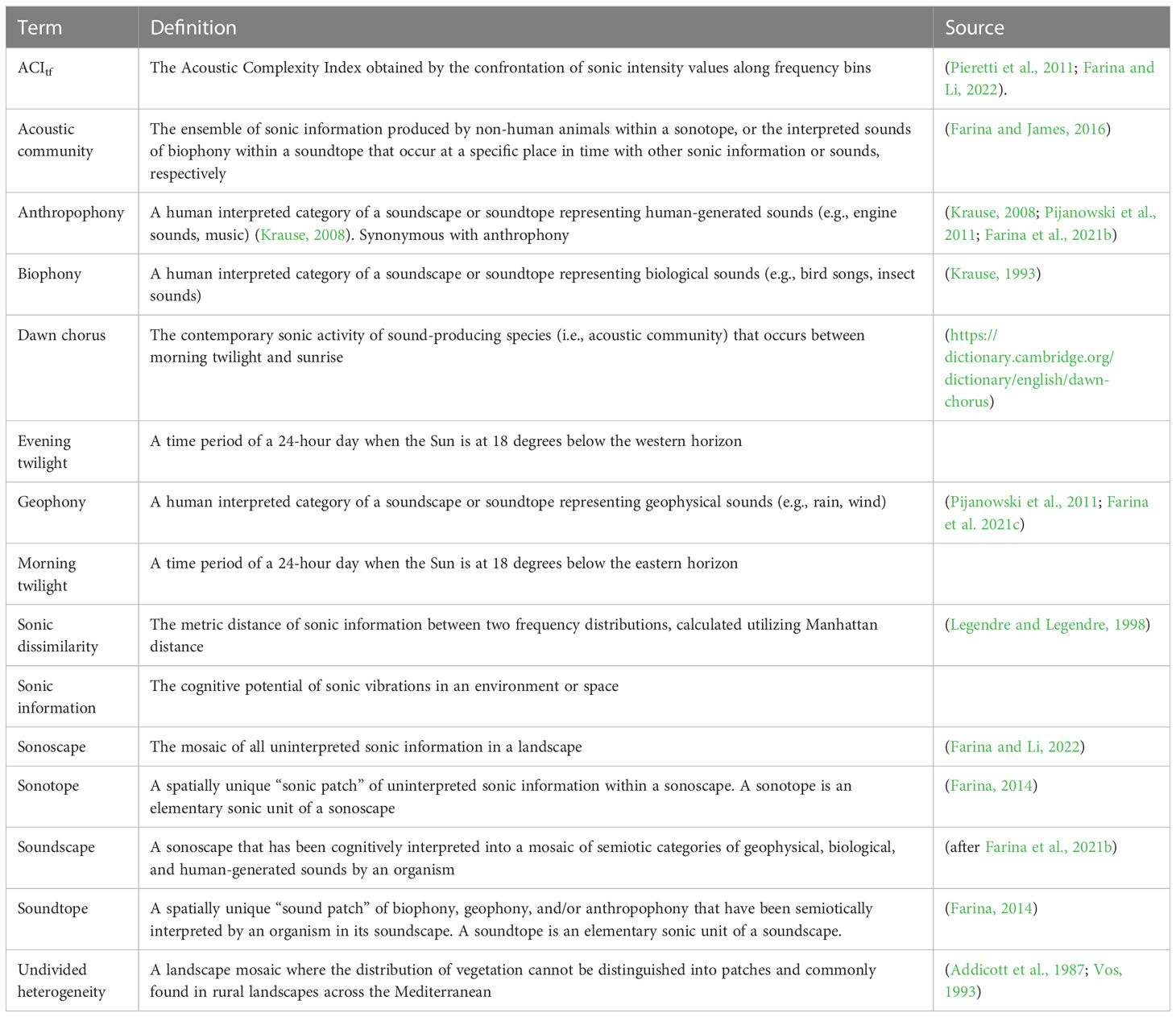
Table 1 Definitions and literature sources of key terms in Ecoacoustics relating to the study of sonotopes.
The concepts and classifications of the sonic environment developed in Ecoacoustics are an attempt to make sense of and explain complex ecological relationships (Farina, 2014; Farina and Gage, 2017). Particularly, much of the theoretical framework and terms of Ecoacoustics in the subfield of soundscape ecology adheres to those analogous to many supported tenants of Landscape Ecology Theory (Pijanowski et al., 2011; Farina, 2014) including patches, ecotopes, temporal patterns, and spatial heterogeneity (Whittaker et al., 1973; Whittaker et al., 1975; Turner, 1989; Juan et al., 2023) (Table 1). However, much of our current understanding of the spatio-temporal attributes of the sonic environment have centered on soundscapes (Krause et al., 2011; Gage and Axel, 2014; Mullet et al., 2016; Aniceto et al., 2022) and acoustic communities (Lellouch et al., 2014; de Camargo et al., 2019; Farina et al., 2021a).
According to Ecoacoustics Theory, all uninterpreted sonic information of a landscape collectively comprise the sonoscape (Farina and Li, 2022). Organisms with the ability to detect sonic information and subsequently interpret the sonoscape into semiotic categories of sounds create a soundscape unique to that organism (Farina and Li, 2022). For humans, soundscapes are generally categorized into biophony (biological sounds), geophony (geophysical sounds), and anthropophony (human-generated sounds) (Krause, 2008; Pijanowski et al., 2011; Farina and Li, 2022).
At finer scales, sonoscapes and soundscapes are comprised of a patchwork of sonotopes and soundtopes, respectively (Farina, 2014). Conceptually, a sonotope is a spatially unique “sonic patch” of uninterpreted sonic information within a sonoscape while a soundtope is a spatially unique “sound patch” of biophony, geophony, and anthropophony that have been semiotically identified by an organism in its soundscape (Farina, 2014). An acoustic community is the aggregate of uninterpreted sonic information produced by non-human animals within a sonotope, or the interpreted sounds of biophony within a soundtope that occur at a specific place in time with other sonic information or sounds, respectively (Farina and James, 2016). According to this hierarchical framework, acoustic communities are nested within a sonotope with all other uninterpreted sonic information that forms a sonic patch that combine with other sonotopes to form a sonoscape. Similarly, the interpreted sounds of acoustic communities combine with geophony and anthropophony within a soundtope, forming a sound patch that combines with other soundtopes to form an organism’s uniquely interpreted soundscape (Table 1).
Unfortunately, the scarcity of empirical evidence has relegated sonotopes and soundtopes as mere speculation rather than as tested hypotheses (Hedfors and Berg, 2003; Farina et al., 2021b). Consequently, there is sufficient need to explore sonotopes and soundtopes, defined by Farina (2014), to test whether evidence supports these concepts and how they are expressed in the contexts of sonoscapes, soundscapes, and acoustic communities. Based on this premise, we hypothesized that a spatially explicit sample of sonic information, acquired from multiple automated recording devices placed in a heterogeneous landscape, would reveal spatially unique sonotopes with distinct patterns over time.
Our objectives were to:
(1) Conduct acoustic surveys within a spatially explicit sample design of a heterogenous landscape.
(2) Analyze the uninterpreted sonic information of the landscape (sonoscape) with acoustic indices.
(3) Characterize the temporal patterns of the sonoscape.
(4) Empirically describe and visualize the spatio-temporal patterns of sonotopes.
2 Methods and materials
2.1 Study area
We selected a heterogeneous landscape with a mixed agricultural history belonging to the rural terraced systems, “coltura mista,” (Sereni, 1961; Vos, 1993) located in the Fivizzano Commune, Northern Tuscany, Italy (44°14’25” North; 10°03’48” East) (elevation: 250 – 360 m above sea level) on the southwestern slope of Tergagliana Mount (Figure 1). We overlaid a 48-ha rectangle over a satellite image of this region in GoogleEarth™ (Google LLC, Mountain View, California, USA) to define the extent of our study area with the intention of sampling a spatially explicit environment characterized by landcover types that conformed to an undivided heterogenous landscape common to this region (Addicott et al., 1987; Vos, 1993). We identified 10 landcover classes that included dense woodlots (24%), tall shrubland (22%), cultivated olive (Olea europaea) groves (20%), abandoned olive groves (13%), unidentified cultivated cropland (7%), grassland (5%), abandoned cropland (5%), abandoned vineyard (4%), cultivated vineyard (1%), and bramble shrubland (<1%).
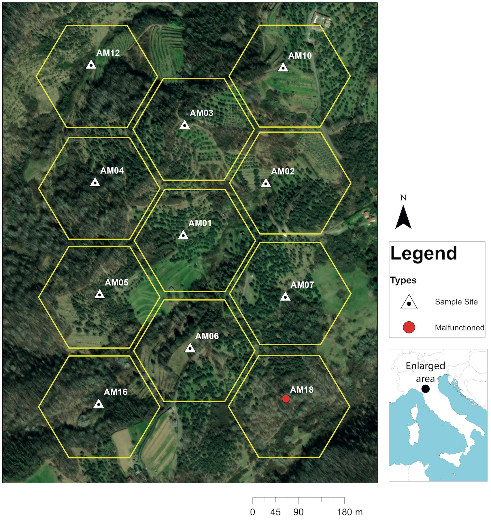
Figure 1 Satellite image of the 48-ha study area representing an undivided heterogenous landscape of mixed land use belonging to the rural terraced systems, “coltura mista,” (Sereni, 1961; Vos, 1993) located in the Fivizzano Commune, Northern Tuscany, Italy (44°14’25” North; 10°03’48” East) overlaid with 11, 4-ha hexagonal cells where sound recording stations were placed approximately 180 m apart.
Our study spanned the seasonal periods of spring to summer (March – July) and late summer to fall (August – November) of 2021. Temperatures ranged from 5.4 – 26.8°C (Mean = 16.7°C) from March – July and 12.7 – 29.6°C (Mean = 19.5°C) from August – November. Precipitation ranged from 0 – 41.8 cm (Mean = 2.3 cm) and 0 – 97.4 cm (Mean = 4.3 cm) over the same time frames, respectively. Wind speeds ranged from 1.0 – 17.2 km/h (Mean = 6.7 km/h) March – July and 3.9 – 13.7 km/h (Mean = 7.7 km/h) August – November.
2.2 Sample design
Because sonic waves in a terrestrial environment attenuate at various distances depending on the amplitude and frequency of the source and characteristics of vegetation and landcover types, it is difficult to determine a precise distance that ensures there is spatial independence between sample sites (Yip et al., 2017a). Coupled with this challenge are weather variables and a recorder’s capability to detect sounds at various distances (Yip et al., 2017b; Darras et al., 2018). For these reasons, recorder sensitivity, distance between microphones, and environment must be carefully considered so that each sample site serves as an independent measure to determine the spatial uniqueness of a sonotope (Farina and Li, 2022). While weather variables cannot be controlled, adjusting the gain of a sound recorder provides a means to control a microphone’s detection sensitivity (Rumsey and McCormicj, 1992; Hill et al., 2019). For distances, Yip et al. (2017b) has shown that 180 m is an appropriate distance for independently detecting a variety of birds in various landcover types (Yip et al., 2017b). The caveat to this is that low frequency bird calls (e.g., owls, ravens) and geophonies may be detected at greater distances depending on the amplitude of the sound source (Yip et al., 2017b). Although these low-frequency soniferous species are rare in our study area, we expected the effects of geophonies would reveal themselves through acoustic analysis.
Following methods described by Farina and Li, 2022 (pp 22 – 25), we overlaid a net of 11, 4-ha hexagonal cells over our 48-ha study area in GoogleEarth as a framework for ensuring spatial independence of sample sites (Figure 1). We then placed a point within the center of each hexagon spaced 180 m apart (Yip et al., 2017b) and utilized their geographic coordinates as a spatial reference for placing recorders in the field. We deployed 11 Audiomoth (AM) recorders (version 1.2.0) (Hill et al., 2019) between 5 – 15 m from pre-assigned coordinates, depending on the location of suitable mounting sites (Figure 1). This variation in distance did not negatively affect the spatial independence of our sample (Yip et al., 2017b; Farina, 2018).
Each recorder was given a unique number (e.g., AM01, AM02) and mounted 1.2 m above the ground on the trunks of trees. Recorders were programmed to sample the ambient sonic environment, with medium-low microphone gain (28.7 db) (Hill et al., 2019), at a sample rate of 32,000 Hz. Recorders were scheduled to run for 5 minutes, pausing for 60 seconds between recordings, over a 24-h period (00:00 to 24:00), totaling 240 files a day between 09 March to 11 November 2021. Sonic data were saved in WAV audio format.
2.2 Landcover assessment
We conducted aerial surveys and took orthophotos at each recording site using a DJI™ Mini 2 Drone with DJI Fly ™ version 1.5.10 for IOS systems (DJI Sky City, Shenzhen, China), flown at 120 m above ground level. We then created a georeferenced orthomosaic for each recording site from 20 – 30 photos in WebODM® (OpenDroneMap™) (https://www.opendronemap.org/webodm). We overlaid a grid of 64, 12.5 x 12.5 m cells over the orthomosaic of our study area and identified the presence or absence of each of the 10 landcover classes within each cell. We calculated the total number of each landcover class for cells with presences that occurred within each hexagonal sample unit. We used these values to represent the frequency of landcover class occurrence and landscape composition within our 11 sample sites.
2.3 Data analysis
2.3.1 Data processing and acoustic indices
We used the Acoustic Complexity Index (ACI) (Pieretti et al., 2011), ACItf, after Farina and Li (2022), as the quantifiable measure of sonic information of a WAV file within the frequency range of 0 – 16,000 Hz. The ACItf is a measure of complexity expressed by all sonic information occurring at intervals (i.e., spectral lines) along a horizontal axis of time (t) and a vertical axis of frequency (f) in a WAV file recorded at a spatially explicit location (i.e., sample site) (Farina and Li, 2022, p 33). As a result, ACItf is an appropriate index for evaluating the sonic characteristics of discrete spatial units of the sonoscape (Sueur et al., 2014; Farina et al., 2016; Cifuentes et al., 2021; Wang et al., 2023).
Acoustic indices were generated using SonoScape™, an open access software operating in MATLAB (Farina and Li, 2022). We calculated ACItf at 1-second intervals for each 5-minute recording across 512 frequency bins separated at 31.25 Hz frequency intervals. An intensity filter was applied to the Fast Fourier Transform matrix to exclude values <0.01 that were generated by internal microphone noise. We also excluded the first six frequency bins from further analysis to avoid confusion caused by the low-frequency vibrations generated by recording devices.
We calculated Sonic Dissimilarity (SD) (Sueur et al., 2008; Lellouch et al., 2014) of ACItf across 506 frequency bins (218 – 16,000 Hz) utilizing Manhattan distance (Legendre and Legendre, 1998) and applied the Hill Evenness (Hill, 1973) to SD Entropy (Shannon and Weaver, 1949) to calculate a single index (0 – 1) of Sonic Dissimilarity Evenness (SDj') among all recording stations in our study area. Within a spatial context, an SDj' value close to one indicates the sonic information of the study area is more similar, or sonically homogenous. Conversely, an SDj' value closer to zero indicates the sonic information of a study area is more dissimilar (i.e., sonically heterogenous). While SDj' is intended to be used to compare two or more study areas, we attempted to apply it across our study area as a measurable indicator of sonic hetero- or homogeneity.
2.3.2 Landcover analysis
We conducted a cluster analysis of landcover classes in Minitab 21.2 (Minitab, LLC. State College, PA) using the Cluster Observation tool. We applied the Ward linkage method, Manhattan distance, and set the number of clusters to one to produce a dendrogram displaying the similarities of landcover class frequencies between sample sites. The cluster analysis enabled us to determine the landcover representation of our sample sites.
2.3.3 Temporal analysis of the sonoscape
When considering sonic information in the context of time, one must consider factors that can affect the sonic environment over the course of a 24-h day and between seasons. There is evidence that several soniferous species synchronize their sonic activities according to the sun cycle (Malavasi and Farina, 2013; Farina et al., 2015). Gil and Llusia (2020) have also found that the dawn chorus of birds in the Mediterranean region begins at astronomical twilight and ends at sunrise. Soniferous nocturnal species of insects and nightingales (Luscinia megarhynchos) have also shown temporal changes in sonic activity depending on the time of night (Hultsch and Todt, 1982; Römer, 2020). Farina (1997) documented that the breeding season of birds in the Mediterranean region largely coincides with the months between March and July.
Based on these observations, we grouped our data into distinct temporal periods over a 24-h day and seasonally. Subsequently, we analyzed our data according to the seasonal periods: spring to summer (March – July) and late summer to fall (August – November). We divided the 24-h day into five astronomical periods: (1) Night I (00:00 [midnight] to morning twilight when the Sun is at 18 degrees below the horizon); (2) Morning Twilight (morning twilight to sunrise); (3) Day (sunrise to sunset), (4) Evening Twilight (sunset to evening twilight when the Sun is 18 degrees below the horizon) and (5) Night II (evening twilight to 00:00 [midnight]) (Figure 2).
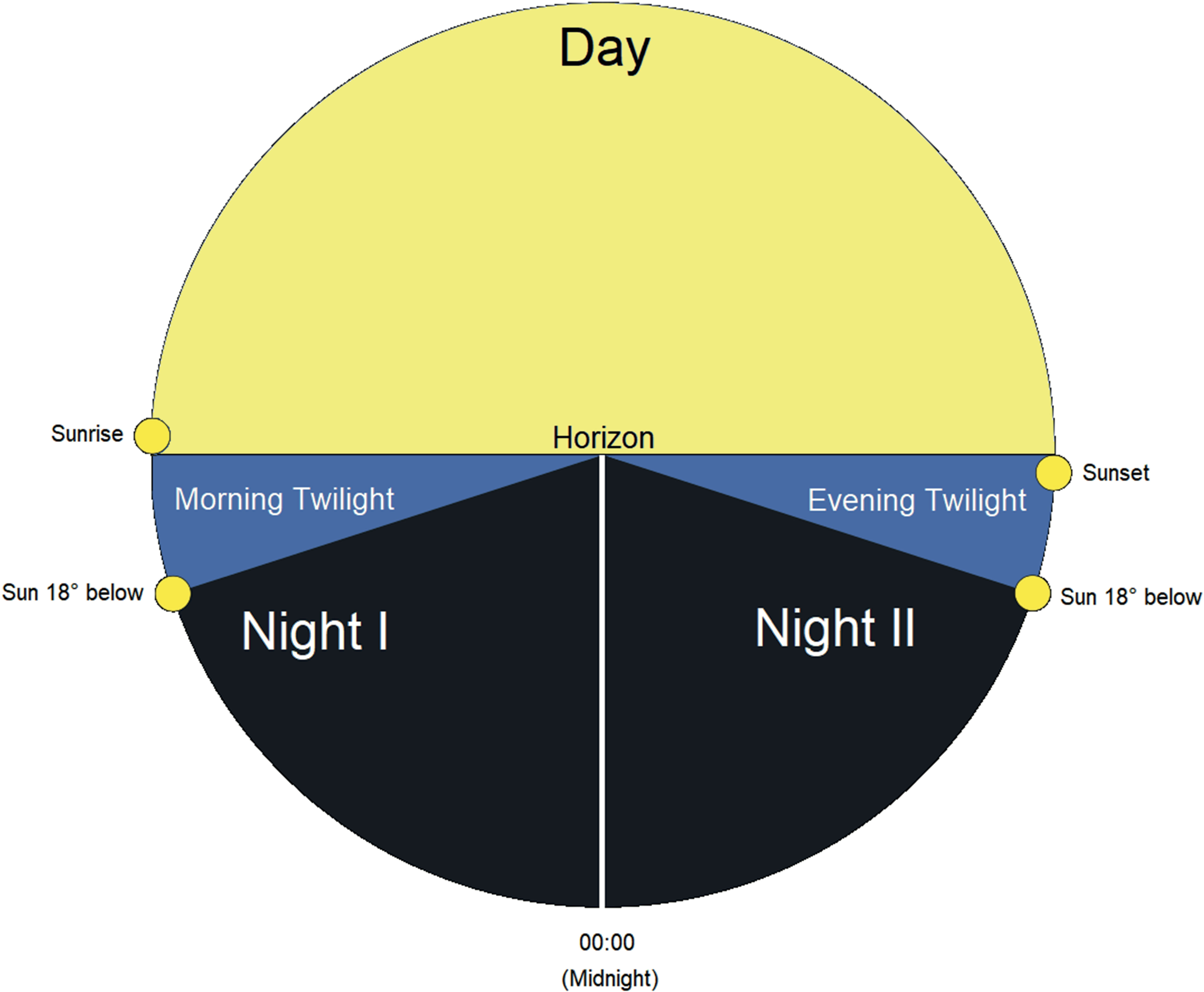
Figure 2 Illustration of the five astronomical temporal periods of a 24-h day including Night I, Morning Twilight, Day, Evening Twilight, and Night II.
Since recordings were synchronized with the ephemeris, we assigned each recording a code from 1 – 5 according to their respective astronomical period. Astronomical data were acquired for every day of sampling using the online ephemeris application http://wave.surfreport.it/. We then visualized the temporal patterns of ACItf across 1-kHz frequency bins spanning 0 – 16,000 Hz according to the five astronomical periods for each recording station separated by season (March – July and August – November). We assessed the differences in total ACItf between seasons using box plots.
2.3.4 Spatio-temporal acoustic analysis
We associated the spatial relationship of sonotopes with time by generating a cluster analysis of total ACItf for each recording station according to astronomical period and season. We applied a similar cluster analysis, as described above, to produce dendrograms that determined whether the total ACItf at each recording station was distinct from others during respective astronomical periods and seasons. We expected this analysis would reveal spatially unique sonotopes within our study area in time and provide empirical support of our hypothesis.
We utilized the cluster algorithm for each astronomical period and season to assign five colors that grouped similarities in total ACItf among recording stations. This method produced a total of 10 dendrograms. We visualized the spatial arrangement of these results by filling each hexagon associated with a recording station with their respective color group in Windows 11 Microsoft Paint. Although the colors of assigned groups were independent between dendrograms, this method presented a visual illustration of how sonotopes were spatially configured in our study area during specific astronomical periods of a 24-h day between two distinct seasonal timeframes.
We calculated the SDj' as an index representing sonic dissimilarity across all recording stations for each astronomical period and season. In this way, the presence of sonotopes could be empirically confirmed through SDj' with an assigned index value indicating the measure of heterogeneity within our study area.
Using the dendextend package and cor.dendlist function (Kassambara, 2017) in R (R Core Team, 2023), we tested the measure of association (i.e., similarity) between dendrograms of ACItf vs. landcover and ACItf vs. ACItf (between astronomical periods within seasons) using Goodman-Kruskal gamma coefficient (γ) (Baker, 1974). We calculated a Sign test to determine if groupings between seasons were statistically different (α = 0.05). These results made it possible to determine whether sonic patterns were associated with landcover (i.e., γ near 1 or -1) and if the arrangement of sonotopes were empirically distinct between astronomical periods and between seasons (i.e., γ near 0).
3 Results
3.1 Sound sampling and landcover representation
Ten out of our 11 recorders operated for an average of 163 days between 09 March – 11 November 2021. Despite one recorder malfunctioning (Figure 1) and days of data being lost due to loss of battery life, we acquired a total of 32,660 hours of recordings. All 10 landcover types were unevenly represented across our sample areas with some sites displaying similarities in composition (Figure 3). Sites AM01 and AM10 displayed similarities largely due to their dominance of grasslands, cropland, and woodlots (Figure 3). Sites AM04 and AM05 displayed a higher dominance of woodlots than other sites while AM02, AM07, and AM03 contained a higher dominance of olive groves (Figure 3). Sites AM06, AM16, and AM12 possessed a higher dominance of tall shrubland than all other sample sites (Figure 3). There was no statistical association between ACItf and landcover (γ = 0.08).
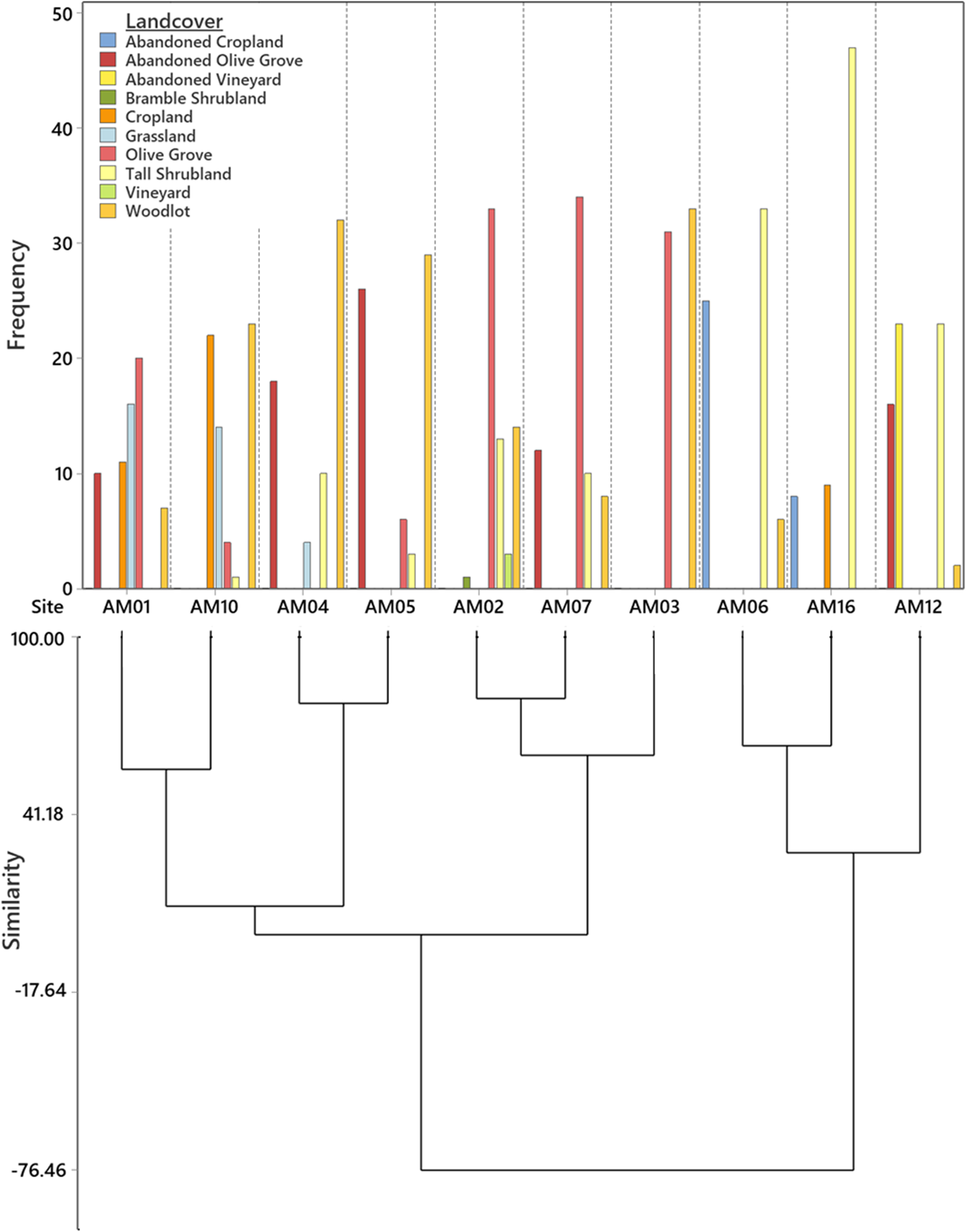
Figure 3 Frequency distribution and cluster analysis (dendrogram) illustrating the composition and representation of 10 landcover classes arranged among 10 sound sample sites.
3.2 Temporal patterns of the sonoscape
The distribution of ACItf along the five astronomical periods of a 24-h day showed significant differences in sonic activity between seasons (Table S1). Comparatively, sonic activity of March – July was significantly higher during the Day than all other astronomical periods while the opposite was true of sonic activity during August – November when the sonic activity was greater during the crepuscular and nocturnal periods of a 24-h day (Table S1; Figure 4). Within their respective seasons, sonic activity did not markedly differ between Morning and Evening Twilight periods, or between Night I and Night II.
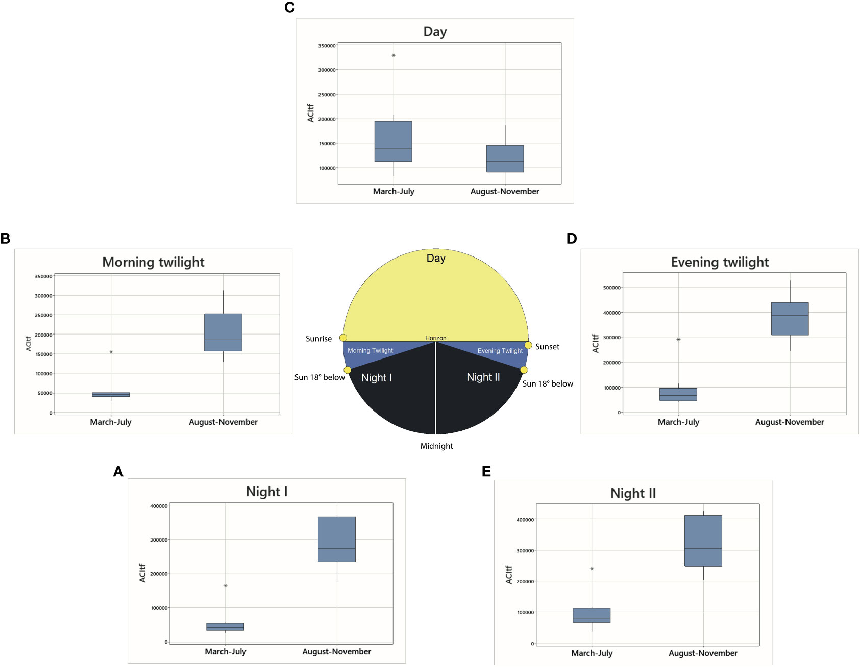
Figure 4 Boxplots of ACItf compared between seasons according to five astronomical periods referenced with Figure 2: (A) Night I, (B) Morning Twilight, (C) Day, (D) Evening Twilight, (E) Night II.
Temporal patterns of ACItf displayed distinct patterns across frequencies when observing individual sample sites within their respective seasons. Most notably, in March – July, AM01, AM02, AM04, and AM10 displayed comparatively lower ACItf values than other sites with some noticeable sonic increases in the mid- to high-frequency ranges during Day, Evening Twilight, and Night II (Figure S1). Sonic activity spiked higher than all other periods for sample sites AM03, AM05, AM06, and AM07 within frequencies <1,000 and >10,000 Hz during Day while other astronomical periods remained comparatively low at the same sites for all frequencies. Sample site AM12 displayed high and similar ACItf values across all frequencies during Day and exhibited a similar peak in sonic activity as AM16 at frequencies between 9,000 – 11,000 Hz during Evening Twilight and Night II (Figure S1). Night I and Morning Twilight appeared to display the lowest comparative ACItf values across all sample sites (Figure S1).
During August – November, all sample sites exhibited a peak in ACItf at 3,000 Hz for all astronomical periods (Figure S1). A second peak of sonic activity was evident between 9,000 – 14,000 Hz for all sample sites, a majority of which occurred during the twilight and night periods (Figure S1). Evening Twilight exhibited ACItf values at AM01, AM04, AM05, AM06, AM07, and AM10. Night I, Night II, and Evening Twilight at AM02 and AM03, displayed similar values within sample sites, albeit different ACItf values between sites (Figure S1). Sample sites AM10 and AM16 exhibited the highest ACItf values of sonic activity than other sites at frequencies between 9,000 and 14,000 Hz. However, this intensity of sonic activity occurred during the astronomical periods of Evening Twilight, Night I and Night II at AM10, and Night II and Morning Twilight, specifically, at AM16. Compared to all other sites, AM16 also displayed the lowest ACItf values during Evening Twilight and highest ACItf values for Morning Twilight and Day within the 9,000 – 14,000 Hz range (Figure S1). All sites displayed the lowest ACItf values between 1,000 – 2,000 and 4,000 – 6,000 Hz (Figure S1).
3.3 Spatio-temporal dynamics of sonotopes
Accounting for the sonic information of all 10 sample sites and frequencies, the sonoscape of our study area during March – July was consistently homogenous (SDj' >0.97) across astronomical periods (Table 2). The sonoscape during August – November was also uniformly homogenous (SDj' >0.95) for Night I, Night II, and Morning Twilight, but comparatively less homogenous during Day (SDj' = 0.69) and Evening Twilight (SDj' = 0.79) (Table 2).
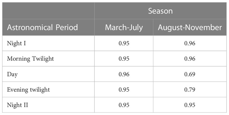
Table 2 Sonic Dissimilarity Evenness (SDj') of the entire study area’s sonoscape compared between seasons and astronomical periods where SDj' values closer to one indicate a more sonic homogenous sonoscape while SDj' values closer to zero indicate a more sonic heterogenous sonoscape.
Although the sonic information of the study area was by and large sonically homogenous, the spatial arrangement and configuration of sonic information within 4-ha sample sites showed remarkable changes according to astronomical period and between seasons.
Figures 5, 6 visualize how sample sites with similar ACItf were grouped into clusters (sonotopes) of a dendrogram, coded by color, and arranged in space over astronomical periods within their respective seasons. Although the colors of any given cluster are arbitrary when compared between astronomical periods, they are meaningful within each astronomical period because they reveal sonic similarities in space and time. Compared between seasons, AM01 and AM12 consistently remained unchanged, despite astronomical period. Notably, AM12 was never grouped with other sample sites representing a unique and static 4-ha sonotope within our study area.
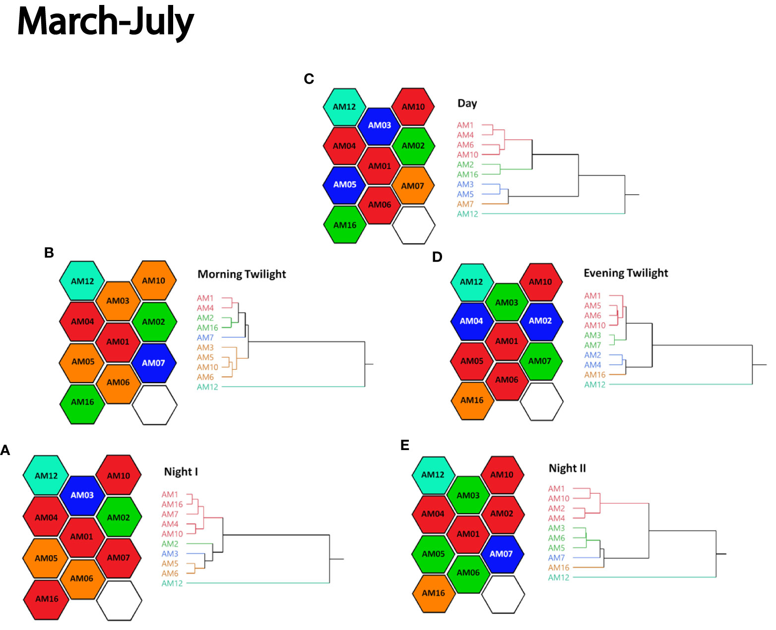
Figure 5 Cluster analysis dendrograms of ACItf grouped by similarity into five color-coded clusters paired with the spatial configuration of respectively colored 4-ha hexagons sample sites representing sonotopes according to five astronomical periods of (A) Night I, (B) Morning Twilight, (C) Day, (D) Evening Twilight, and (E) Night II in March – July 2021. Sonotope colors represent similarities within astronomical periods but are independent between astronomical periods.
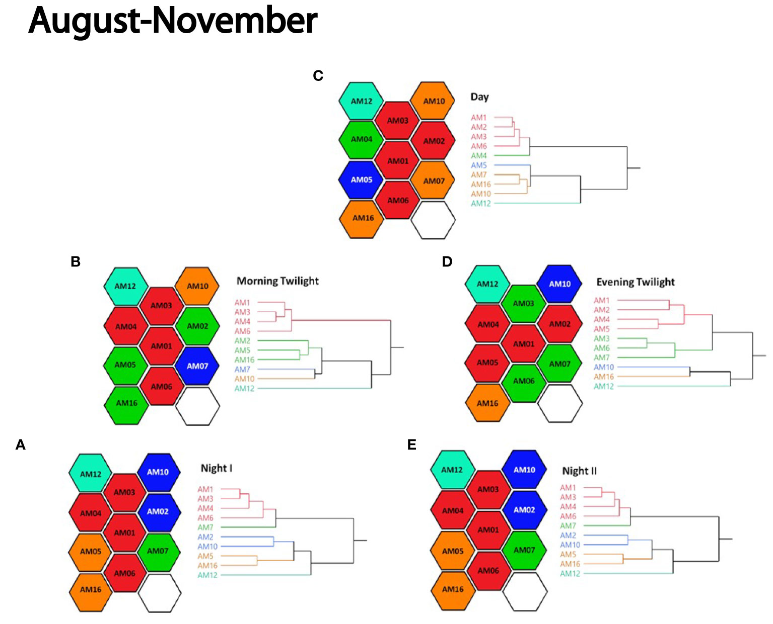
Figure 6 Cluster analysis dendrograms of ACItf grouped by similarity into five color-coded clusters paired with the spatial configuration of respectively colored 4-ha hexagons sample sites representing sonotopes according to five astronomical periods of (A) Night I, (B) Morning Twilight, (C) Day, (D) Evening Twilight, and (E) Night II in August-November 2021. Sonotope colors represent similarities within astronomical periods but are independent between astronomical periods.
More generally, sonotopes not only changed the arrangement in which they shared similar ACItf between sample sites, they also changed their size and configuration during astronomical periods. While this was true for all astronomical periods in March – July (Figure 5), the periods of Night I and Night II of August – November did not change sonotope arrangements or ACItf groupings (Figure 6). In some cases, sample sites exhibited unique and isolated 4-ha sonotopes depending on astronomical period (Figure 5) (e.g., March – July: Night I [AM03]; Morning Twilight and Day [AM07]; Evening Twilight and Night II [AM16]). In other cases, sonotopes had similar ACItf values with two or more adjacent sample sites, creating larger sonotopes ranging from 8 – 16 ha sonotopes configured in a variety of arrangements (Figure 6) (e.g., August – November: Night I, Night II, and Morning Twilight [AM05 + AM16]; Night I, Night II, and Morning Twilight [AM01 + AM03 + AM04 + AM06]). There were also astronomical periods when sonotopes possessed similar ACItf values with others but were spatially disjunct from one another (Figure 5) (e.g., March – July: Day [AM03 – AM05]; Evening Twilight [AM03 – AM07]).
During March – July, the adjacent sample sites AM01 and AM04 were consistently grouped during Night I, Morning Twilight, Day, and Night II (Figure 5). Adjacent sample sites AM05 and AM06 were also consistently grouped together in March – July although their colored grouping shifted during Night II (Figure 5). Adjacent sample sites AM01, AM03, and AM06 were consistently grouped together during all astronomical periods except Evening Twilight during August – November (Figure 6). The adjacent sample sites AM05 and AM16 were consistently grouped for the periods of Night I, Night II, and Morning Twilight (Figure 6).
When compared between astronomical periods, dendrogram arrangements of sonotope clusters in March – July ranged from moderately associated (γ = 0.47) to relatively strong (γ = 0.68) (Table 3). Conversely, dendrogram arrangements of sonotopes between astronomical periods in August – November ranged from weakly associated (γ = 0.32) to negligible (γ = 0.04) apart from Night I and Night II dendrograms that exhibited very strong associations to one another (γ = 0.99) (Table 3). Generally, sonotope arrangements in March – July were significantly different than those in August – November (p < 0.02).
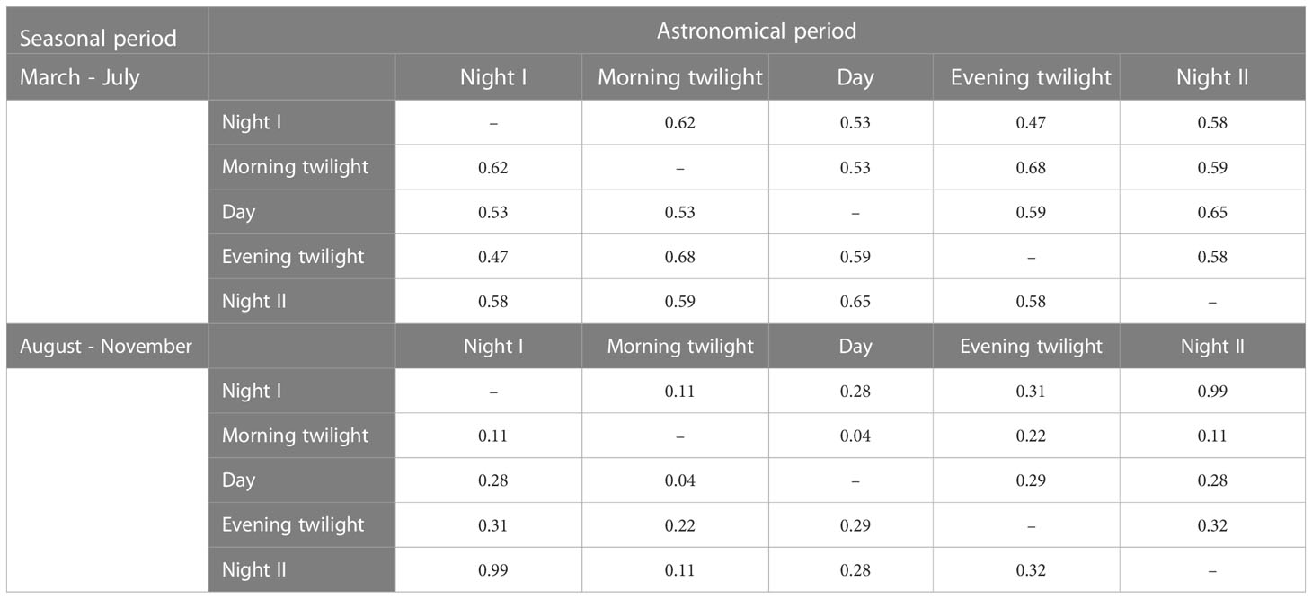
Table 3 Goodman-Kruskal gamma coefficient (γ) comparing dendrograms of ACItf across astronomical periods within their respective seasons. Values closer to zero indicate dendrograms are more similar while values closer to one indicate dendrograms are more distinct.
4 Discussion
There has been some effort to conceptualize and characterize the spatial and temporal patterns of soundscapes (Truax and Barrett, 2011; Fuller et al., 2015; Mullet et al., 2016; Putland et al., 2017) and understand the nature of acoustic communities (Farina and James, 2016; Farina et al., 2021a; Hao et al., 2021). Considering soundscapes and acoustic communities represent the very coarse and fine scales of a human-interpreted sonic environment, respectively, there remains a missing link between these two scales and the context for their ecological significance. Sonotopes and soundtopes, introduced by Farina (2014), provide a conceptual hypothesis that fills the information and relationship gaps between soundscapes and acoustic communities.
Here, we refrained from using our own interpretation of sounds within our study area and instead we analyzed and evaluated the sonic information of the landscape as a singular sonoscape. We employed a spatially explicit and representative sample design (Farina and Li, 2022) of an undivided heterogenous, rural, Italian landscape where sonotopes would most likely be revealed using ACItf and SDj'. Temporally, we found empirical evidence that the sonoscape exhibited differences in sonic activity between seasons and distinct patterns in accordance with five specific astronomical periods of a 24-h day. Spatially, we discovered that the sonoscape was comprised of a dynamic sonic patchwork of sonotopes that exhibited distinct arrangements and configurations of size and place depending on the season and astronomical period.
We found no matching correspondence among our sound sample stations when comparing dendrograms of landcover and ACItf. While large-scale studies have found links between landcover and soundscape metrics (Pijanowski et al., 2011; Fuller et al., 2015; Mullet et al., 2016; Mullet et al., 2017), the spatial scale of our study area and the convoluted vegetation dynamics that occur between land use practices and landcover types makes a direct link to sonic phenomena unclear and problematic (Farina and Fuller, 2017; Gasc et al., 2018).
The temporal patterns that emerged throughout this sonoscape can be attributed to the spatio-temporal dominance of sonic information produced by biophonies within acoustic communities (Farina and James, 2016). Accordingly, the temporal variability we observed in ACItf (a proxy of sonic activity (Wang et al., 2023) between the seasons and astronomical periods indicated distinct differences in sonic activity generated by the biophony of birds in March – July and the chorus of tree cricket (Oecanthus pellucens (Scopoli, 1763)) and Bushcricket (Tettigonia viridissima (Linnaeus, 1758)) in August – November. The reason why ACItf was predominantly higher during the astronomical period of Day could be explained by the fact that birds are known to synchronize their sonic activities with the sun cycle (Malavasi and Farina, 2013; Farina et al., 2015; Gil and Llusia, 2020). Similarly, birds of this region have been documented to be more active during the Mach – July breeding season (Farina, 1997). Alternatively, the biophonies of birds in this region are known to decline in August (Farina, 1997) at which time we documented a rise in ACItf during crepuscular and nocturnal periods attributed to cricket biophonies in August – November. This would explain why the arrangement of sonotopes were significantly different between seasons.
When evaluated across frequencies, we generally documented relatively higher values of ACItf and sonic activity in March – July at mid- to high frequencies, and two distinct peaks in ACItf in August – November at 3,000 Hz and 9,000 – 14,000 Hz. Considering sonic activity at frequencies >2,000 Hz are often attributed to biophony (Gage and Axel, 2014; Mullet, 2020), our data suggests a predominance of mid- to high frequency biophonies contributing to this soundscape. We not only observed differential temporal patterns at these frequencies across our entire study area, but we also documented distinct temporal patterns at individual sample sites suggesting the occurrence of acoustic communities that are intimately influenced by seasonal and astronomical periods. Although data variation between sample sites in a landscape is expected (Khosla et al., 2010), this temporal analysis of individual recording stations revealed preliminary evidence that our spatially independent sample sites exhibited sonotope characteristics within a sonoscape that links to the behaviors of acoustic communities (Farina and James, 2016; Farina et al., 2021a; Hao et al., 2021).
Sonic Dissimilarity Evenness (SDj') indicated that our sonoscape was sonically homogenous between seasons and across astronomical periods. Contrary to what we expected, SDj' did not support evidence of a sonically heterogeneous sonoscape even though we identified distinct sonotopes from cluster analyses. This is likely due, in part, to the scale of SDj'’s inference. Since SDj' calculates the evenness of ACItf across all recording stations, it provides an index generalizing the sonic conditions of the entire sonoscape over time, space, and frequencies (Farina and Li, 2022). While we argue that SDj' remains a relevant index to compare two or more sonoscapes, we found that the index is not sensitive to the finer scale variations found between and among individual sample sites that we captured in cluster analyses. We encourage further research on the application of SDj' in Ecoacoustics.
We discovered strong evidence of sonotopes occurring within our study area based on cluster analyses of ACItf segmented according to astronomical period and season. Dendrograms and group classifications of the cluster analyses enabled us to statistically identify sample sites with distinct and similar ACItf indicative of sonotopes. However, the color coordinated map of our 10, 4-ha hexagonal sample sites revealed that sonotopes displayed dynamic spatio-temporal patterns across astronomical periods and seasons as individual units and study area-wide configurations. The differences and similarities of ACItf between and among sonotopes created small distinct sonic patches and larger sonic patches that changed their sonic signatures (i.e., characteristics) over time, simultaneously changing the spatial arrangement of the sonoscape.
The causation of this spatio-temporal dynamic is not fully understood. Yet, we speculate that the spatial arrangement of acoustic communities and the temporal changes in their biophonies that we observed occurring between seasons and across astronomical periods likely contributed to the behavior of sonotopes. Conversely, sonotopes in our study area that were static and recurrent over time are likely a result of continuous geophonies generated by a local stream (Farina et al., 2021c). In this way, acoustic communities and continuous geophonies play an important role in the arrangement of sonotopes and the overall composition, patterns, and processes of the sonoscape (Pijanowski et al., 2011). We strongly encourage further study to explain these ecological relationships.
5 Conclusions
We applied a sampling methodology and applicable acoustic indices (Farina and Li, 2022) to a sonoscape in rural Italy that considered landscape characteristics, seasonality, astronomical period, and distance to test the hypothesis that this sonoscape consists of a nested arrangement of distinct sonotopes. Our results clearly support this hypothesis, providing further evidence that the sonic information composing a sonoscape exhibits temporal patterns between seasons and across astronomical periods of a 24-h day. We found that the dynamic spatial arrangements and configuration of sonotopes within the sonoscape are also closely tied to seasonal and astronomical periods due to the presence and sonic behavior of acoustic communities.
We recommend that further ecoacoustic studies acknowledge and continue to investigate the influence of astronomical periods on sonoscapes, sonotopes, and acoustic communities. We also encourage others to identify the sound sources of sonoscapes and sonotopes to more clearly understand how biophony, geophony, and anthropophony contribute to the compositions, patterns, and processes of soundtopes.
Data availability statement
The original contributions presented in the study are included in the article/Supplementary Material. Further inquiries can be directed to the corresponding author.
Author contributions
AF and TM developed the theoretical basis of this manuscript and contributed equally to the literature review, writing, and revisions of the manuscript. AF conducted all field work and data processing. AF and TM contributed equally to the interpretation of results. TB, PS, and TT provided institutional and financial support and the motivation to develop and publish this work. PL contributed to technical support for data processing. All authors contributed to the successful completion and publication of this article and collectively approved the submitted version.
Acknowledgments
We are thankful to our families and colleagues who have supported our work. We appreciate the peer reviewers and editor for helping us improve our manuscript for a wider readership. We kindly dedicate our work with respect and remembrance to our friend and colleague, Giani Pavan.
Conflict of interest
The authors declare that the research was conducted in the absence of any commercial or financial relationships that could be construed as a potential conflict of interest.
Publisher’s note
All claims expressed in this article are solely those of the authors and do not necessarily represent those of their affiliated organizations, or those of the publisher, the editors and the reviewers. Any product that may be evaluated in this article, or claim that may be made by its manufacturer, is not guaranteed or endorsed by the publisher.
Author disclaimer
The findings and conclusions in this article are those of the authors and do not necessarily represent the views of any government agencies. Any use of trade, product, or firm names is for descriptive purposes only and does not imply endorsement by the US government.
Supplementary material
The Supplementary Material for this article can be found online at: https://www.frontiersin.org/articles/10.3389/fevo.2023.1205272/full#supplementary-material
References
Addicott J. F., Aho J. M., Antolin M. F., Padilla D. K., Richardson J. S., Soluk D. A. (1987). Ecological neighborhoods: scaling environmental patterns. Oikos 49, 340–346. doi: 10.2307/3565770
Aniceto A. S., Ferguson E. L., Pedersen G., Tarroux A., Primicerio R. (2022). Temporal patterns in the soundscape of a Norwegian gateway to the Arctic. Sci. Rep. 12 (1), 7655. doi: 10.1038/s41598-022-11183-y
Baker F. B. (1974). Stability of two hierarchical grouping techniques case I: sensitivity to data errors. J. Am. Stat. Assoc. 69 (346), 440–445. doi: 10.2307/2285675
Cifuentes E., Vélez Gómez J., Butler S. J. (2021). Relationship between acoustic indices, length of recordings and processing time: a methodological test. Biota Colomb. 22 (1), 26–35. doi: 10.21068/c2021.v22n01a02
Core Team R. (2023). R: A Language and Environment of Statistical Computing (Vienna, Austria: R Foundation for Statistical Computing). Available at: https://www.R-project.org/.
Darras K., Furnas B., Fitriawan I., Mulyani Y., Tscharntke T. (2018). Estimating bird detection distances in sound recordings for standardizing detection ranges and distance sampling. Methods Ecol. Evol. 9 (9), 1928–1938. doi: 10.1111/2041-210X.13031
de Camargo U., Roslin T., Ovaskainen O. (2019). Spatio-temporal scaling of biodiversity in acoustic tropical bird communities. Ecography 42 (11), 1936–1947. doi: 10.1111/ecog.04544
Farina A. (1997). Landscape structure and breeding bird distribution in a sub-Mediterranean agro-ecosystem. Landscape Ecol. 12, 365–378. doi: 10.1023/A:1007934518160
Farina A. (2000). Landscape ecology in action (Dordrecht, The Netherlands: Springer Science & Business Media).
Farina A. (2014). Soundscape ecology: principles, patterns, methods and applications (Dordrecht, The Netherlands: Springer Science & Business Media).
Farina A. (2018). Perspectives in ecoacoustics: A contribution to defining a discipline. journal of ecoacoustics. J. Ecoacoustic 2, #TRZD5I. doi: 10.22261/JEA.TRZD5I
Farina A., James P. (2016). The acoustic communities: Definition, description and ecological role. Biosystems 147, 11–20. doi: 10.1016/j.biosystems.2016.05.011
Farina A., Fuller S. (2017). Landscape patterns and soundscape processes. Ecoacoust.: Ecol. Role Sounds, 193–209. doi: 10.1002/9781119230724.ch11
Farina A., Gage S. H. (2017). Ecoacoustics: The ecological role of sounds (Oxford, UK: John Wiley & Sons).
Farina A., Li P. (2022). Methods in ecoacoustics. The Acoustic Complexity Index (Cham, Switzerland: Springer Nature).
Farina A., Ceraulo M., Bobryk C., Pieretti N., Quinci E., Lattanzi E. (2015). Spatial and temporal variation of bird dawn chorus and successive acoustic morning activity in a Mediterranean landscape. Bioacoustics 24 (3), 269–288. doi: 10.1080/09524622.2015.1070282
Farina A., Pieretti N., Salutari P., Tognari E., Lombardi A. (2016). The application of the acoustic complexity indices (ACI) to ecoacoustic event detection and identification (EEDI) modeling. Biosemiotics 9, 227–246. doi: 10.1007/s12304-016-9266-3
Farina A., Righini R., Fuller S., Li P., Pavan G. (2021a). Acoustic complexity indices reveal the acoustic communities of the old-growth Mediterranean forest of Sasso Fratino Integral Natural Reserve (Central Italy). Ecol. Indic. 120, 106927. doi: 10.1016/j.ecolind.2020.106927
Farina A., Eldridge A., Li P. (2021b). Ecoacoustics and multispecies semiosis: Naming, semantics, semiotic characteristics, and competencies. Biosemiotics 14 (1), 141–165. doi: 10.1007/s12304-021-09402-6
Farina A., Mullet T. C., Bazarbayeva T. A., Tazhibayeva T., Bulatova D., Li P. (2021c). Perspectives on the ecological role of geophysical sounds. Front. Ecol. Evol. 9, 748398. doi: 10.3389/fevo.2021.748398
Fuller S., Axel A. C., Tucker D., Gage S. H. (2015). Connecting soundscape to landscape: Which acoustic index best describes landscape configuration? Ecol. Indic. 58, 207–215. doi: 10.1016/j.ecolind.2015.05.057
Gage S. H., Axel A. C. (2014). Visualization of temporal change in soundscape power of a Michigan lake habitat over a 4-year period. Ecol. Inf. 21, 100–109. doi: 10.1016/j.ecoinf.2013.11.004
Gasc A., Gottesman B. L., FrancOmano D., Jung J., Durham M., Mateljak J., et al. (2018). Soundscapes reveal disturbance impacts: biophonic response to wildfire in the Sonoran Desert Sky Islands. Landscape Ecol. 33, 1399–1415. doi: 10.1007/s10980-018-0675-3
Gil D., Llusia D. (2020). The bird dawn chorus revisited. Coding strategies vertebrate acoustic Communicat., 45–90. doi: 10.1007/978-3-030-39200-0_3
Hao Z., Wang C., Sun Z., Zhao D., Sun B., Wang H., et al. (2021). Vegetation structure and temporality influence the dominance, diversity, and composition of forest acoustic communities. For. Ecol. Manage. 482, 118871. doi: 10.1016/j.foreco.2020.118871
Hedfors P., Berg P. G. (2003). The sounds of two landscape settings: auditory concepts for physical planning and design. Landscape Res. 28 (3), 245–263. doi: 10.1080/01426390306524
Hill M. O. (1973). Diversity and evenness: a unifying notation and its consequences. Ecology 54 (2), 427–432. doi: 10.2307/1934352
Hill A. P., Prince P., Snaddon J. L., Doncaster C. P., Rogers A. (2019). AudioMoth: A low-cost acoustic device for monitoring biodiversity and the environment. HardwareX 6, e00073. doi: 10.1016/j.ohx.2019.e00073
Hultsch H., Todt D. (1982). Temporal performance roles during vocal interactions in nightingales (Luscinia megarhynchos B.). Behav. Ecol. Sociobiol. 11, 253–260. doi: 10.1007/BF00299302
Juan W., Junjie L., Chao L., Xiaoyu D., Yong W. (2023). Species niche and interspecific associations alter flora structure along a fertilization gradient in an alpine meadow of Tianshan Mountain, Xinjiang. Ecol. Indic. 147, p.109953. doi: 10.1016/j.ecolind.2023.109953
Kassambara A. (2017). Practical guide to cluster analysis in R: Unsupervised machine learning (Vol. 1) (Sthda). Available at: http://www.sthda.com.
Khosla R., Westfall D. G., Reich R. M., Mahal J. S., Gangloff W. J. (2010). Spatial variation and site-specific management zones. Geostatistical Appl. Precis. Agric., 195–219. doi: 10.1007/978-90-481-9133-8_8
Krause B. L. (1993). The niche hypothesis: a virtual symphony of animal sounds, the origins of musical expression and the health of habitats. Soundscape Newslett. 6, 6–10.
Krause B. (2008). Anatomy of the soundscape: evolving perspectives. J. Audio Eng. Soc. 56, 1/2, 73–80.
Krause B., Gage S. H., Joo W. (2011). Measuring and interpreting the temporal variability in the soundscape at four places in Sequoia National Park. Landscape Ecol. 26, pp.1247–1256. doi: 10.1007/s10980-011-9639-6
Lellouch L., Pavoine S., Jiguet F., Glotin H., Sueur J. (2014). Monitoring temporal change of bird communities with dissimilarity acoustic indices. Methods Ecol. Evol. 5 (6), 495–505. doi: 10.1111/2041-210X.12178
Malavasi R., Farina A. (2013). Neighbours' talk: interspecific choruses among songbirds. Bioacoustics 22 (1), 33–48. doi: 10.1080/09524622.2012.710395
Mullet T. C. (2020). An ecoacoustic snapshot of a subarctic coastal wilderness: Aialik Bay, Alaska 2019. J. Ecoacoust. 4 (1), 2. doi: 10.35995/jea4010002
Mullet T. C., Farina A., Gage S. H. (2017). The acoustic habitat hypothesis: An ecoacoustics perspective on species habitat selection. Biosemiotics 10 (3), 319–336. doi: 10.1007/s12304-017-9288-5
Mullet T. C., Gage S. H., Morton J. M., Huettmann F. (2016). Temporal and spatial variation of a winter soundscape in south-central Alaska. Landscape Ecol. 31, 1117–1137. doi: 10.1007/s10980-015-0323-0
Pieretti N., Farina A., Morri D. (2011). A new methodology to infer the singing activity of an avian community: The Acoustic Complexity Index (ACI). Ecol. Indic. 11 (3), 868–873. doi: 10.1016/j.ecolind.2010.11.005
Pijanowski B. C., Villanueva-Rivera L. J., Dumyahn S. L., Farina A., Krause B. L., Napoletano B. M., et al. (2011). Soundscape ecology: the science of sound in the landscape. BioScience 61 (3), 203–216. doi: 10.1525/bio.2011.61.3.6
Putland R. L., Constantine R., Radford C. A. (2017). Exploring spatial and temporal trends in the soundscape of an ecologically significant embayment. Sci. Rep. 7 (1), p.5713. doi: 10.1038/s41598-017-06347-0
Römer H. (2020). Insect acoustic communication: the role of transmission channel and the sensory system and brain of receivers. Funct. Ecol. 34 (2), 310–321. doi: 10.1111/1365-2435.13321
Ross S. R. J., O'Connell D. P., Deichmann J. L., Desjonquères C., Gasc A., Phillips J. N., et al. (2023). Passive acoustic monitoring provides a fresh perspective on fundamental ecological questions. Funct. Ecol. 37 (4), 959–975. doi: 10.1111/1365-2435.14275
Sueur J., Farina A. (2015). Ecoacoustics: the ecological investigation and interpretation of environmental sound. Biosemiotics 8, 493–502. doi: 10.1007/s12304-015-9248-x
Sueur J., Farina A., Gasc A., Pieretti N., Pavoine S. (2014). Acoustic indices for biodiversity assessment and landscape investigation. Acta Acustica united Acustica 100 (4), 772–781. doi: 10.3813/AAA.918757
Sueur J., Pavoine S., Hamerlynck O., Duvail S. (2008). Rapid acoustic survey for biodiversity appraisal. PloS One 3 (12), e4065. doi: 10.1371/journal.pone.0004065
Truax B., Barrett G. W. (2011). Soundscape in a context of acoustic and landscape ecology. Landscape Ecol. 26, 1201–1207. doi: 10.1007/s10980-011-9644-9
Turner M. G. (1989). Landscape ecology: the effect of pattern on process. Annu. Rev. Ecol. systemat 20 (1), 171–197. doi: 10.1146/annurev.es.20.110189.001131
Vos W. (1993). Recent landscape transformation in the Tuscan Apennines caused by changing land use. Landscape urban Plann. 24, 1–4: 63-68.
Wang Y., Zhang Y., Xia C., Møller A. P. (2023). A meta-analysis of the effects in alpha acoustic indices. Biodiversity Sci. 31 (1), 22369. doi: 10.17520/biods.2022369
Whittaker R. H., Levin S. A., Root R. B. (1973). Niche, habitat, and ecotope. Am. Nat. 107 (955), 321–338. doi: 10.1086/282837
Whittaker R. H., Levin S. A., Root R. B. (1975). On the reasons for distinguishing" niche, habitat, and ecotope". Am. Nat. 109 (968), 479–482. doi: 10.1086/283018
Xie J., Hu K., Zhu M., Guo Y. (2020). Data-driven analysis of global research trends in bioacoustics and ecoacoustics from 1991 to 2018. Ecol. Inf. 57, 101068. doi: 10.1016/j.ecoinf.2020.101068
Yip D. A., Bayne E. M., Sólymos P., Campbell J., Proppe D. (2017a). Sound attenuation in forest and roadside environments: Implications for avian point-count surveys. Condor: Ornithol. Appl. 119 (1), 73–84. doi: 10.1650/CONDOR-16-93.1
Keywords: acoustic community, ecoacoustics, Italy, sonoscape, sonotope, soundscape, soundtope
Citation: Farina A, Mullet TC, Bazarbayeva TA, Tazhibayeva T, Polyakova S and Li P (2023) Sonotopes reveal dynamic spatio-temporal patterns in a rural landscape of Northern Italy. Front. Ecol. Evol. 11:1205272. doi: 10.3389/fevo.2023.1205272
Received: 13 April 2023; Accepted: 25 July 2023;
Published: 22 August 2023.
Edited by:
Juan M. Daza, University of Antioquia, ColombiaReviewed by:
Felipe N. Moreno-Gómez, Universidad Católica del Maule, ChileDarren O’Connell, University College Dublin, Ireland
Copyright © 2023 Farina, Mullet, Bazarbayeva, Tazhibayeva, Polyakova and Li. This is an open-access article distributed under the terms of the Creative Commons Attribution License (CC BY). The use, distribution or reproduction in other forums is permitted, provided the original author(s) and the copyright owner(s) are credited and that the original publication in this journal is cited, in accordance with accepted academic practice. No use, distribution or reproduction is permitted which does not comply with these terms.
*Correspondence: Almo Farina, YWxtby5mYXJpbmFAdW5pdXJiLml0