 Kimberly J. Ledger1,2†
 Yingxin Su3†
 Jong Yoon Jeon4
 Aimee H. Fullerton5
 David Kuligowski5
 Todd Bennett5
 Keith Denton6Michael McHenry7John H. McMillan8Joseph H. Anderson9Heidi Connor10
 Todd R. Seamons9
 George Pess5Krista M. Nichols5
 Garrett McKinney9*Travis Seaborn11,12*Alexandra K. Fraik13*
- 1Department of Wildlife Ecology and Conservation, University of Florida, Gainesville, FL, United States
- 2College of Fisheries and Ocean Sciences, University of Alaska Fairbanks, Fairbanks, AK, United States
- 3Department of Animal Science, University of California, Davis, Davis, CA, United States
- 4Department of Forestry and Natural Resources, Purdue University, West Lafayette, IN, United States
- 5National Oceanic and Atmospheric Administration (NOAA), National Marine Fisheries Service, Northwest Fisheries Science Center, Seattle, WA, United States
- 6K Denton and Associates, LLC, Sequim, WA, United States
- 7Lower Elwha Klallam Tribe, Natural Resources Department, Port Angeles, WA, United States
- 8The Conservation Angler, Edmonds, WA, United States
- 9Washington Department of Fish and Wildlife, Olympia, WA, United States
- 10National Park Service, Olympic National Park, Port Angeles, WA, United States
- 11School of Natural Resource Sciences, North Dakota State University, Fargo, ND, United States
- 12Fish and Wildlife Sciences, University of Idaho, Moscow, ID, United States
- 13National Genomics Center for Wildlife and Fish Conservation, United States Department of Agriculture (USDA) Forest Service, Missoula, MT, United States
Barriers such as hydroelectric dams inhibit migratory pathways essential to many aquatic species, resulting in significant losses of species, their unique life-history forms, and genetic diversity. Understanding the impacts of dam removal to species recovery at these different biological levels is crucial to fully understand the restoration response. We used the removal of two large dams on the Elwha River as an opportunity to characterize how restored connectivity impacts the reestablishment of two fish species, Chinook salmon (Oncorhynchus tshawytscha) and Steelhead/rainbow trout (Oncorhynchus mykiss), and their unique ocean migration return-timing life-history forms. In this study, we employed riverscape genetics to understand how restoration and the environment influence the distribution of neutral and return-timing genetic variation underlying the migratory life-history forms and species at- and between- sampling sites. We genotyped fish sampled over time and space in the Elwha River using Genotyping-in-Thousands by sequencing (GTseq) loci for both species at neutral and putatively adaptive loci in and near the major effect genic region GREB1L/ROCK1 putatively associated with migration timing. We observed little evidence of genetic structure for either species, but a statistically significant increase in early return-timing alleles in upriver O. mykiss population post-dam removal. For O. tshawytscha, at-site genetic variation was shaped by river distance and a combination of environmental habitat differences, while between-site genetic variation was mainly shaped by river distance. For all O. mykiss, at- and between-site genetic variation is primarily explained by river distance. Genetic variation in juvenile and adult Steelhead, respectively, were influenced by at- and between-site environmental and habitat differences. Our study illustrates the power of using genetics to understand the implications of both demography and environment in facilitating the recovery of species and their diverse life-history forms following barrier removal.
1 Introduction
Significant habitat degradation, reduced connectivity, and total isolation of suitable habitat are possible outcomes of anthropogenic barriers in freshwater environments for numerous species (Bunn and Arthington, 2002). Anthropogenic barriers can cause significant population declines, extirpations, and elimination of unique life-histories, which can have cascading ecological effects for the system across taxa (Brenkman et al., 2008; Bellmore et al., 2019; Zarri et al., 2022). Barrier removal has occurred for decades to improve accessibility and reestablish the necessary habitats for migratory animals such as salmon (Pess et al., 2012; Pess et al., 2014; Bellmore et al., 2019), which has in turn has successfully restored connectivity and contributed to population gains for key taxa in formerly blocked habitats (Brenkman et al., 2012; McHenry et al., 2017; Duda et al., 2020; Hess et al., 2020; Fraik et al., 2021; Pess et al., In Review). Understanding the extent to which the removal of these large barriers may ultimately lead to restored biological communities remains an important area of study (Grummer et al., 2019; Tamario et al., 2019).
Necessary ecological conditions for movement must exist for aquatic species to reestablish in their historical habitat after barrier removal. Aquatic species respond, move and disperse across riverscapes in different ways, as a function of their migration capabilities (Crozier et al., 2008; Dodson et al., 2013; Pess et al., 2014). Some species remain in one freshwater habitat for their entire lives, whereas others move between different freshwater environments (e.g., rivers and lakes) or into marine habitats (Quinn, 2018). This is exemplified in salmonids which undergo physiological transformations to migrate (Nichols et al., 2008; Hecht et al., 2012; Dodson et al., 2013; Kendall et al., 2015) and have significant intraspecific variation in their migration life-history forms. Challenges to upriver movement in freshwater environments for salmonid species include the distance to new habitat, environmental conditions, physical capacity to reach the habitat, life-history traits required to exploit the habitat, and physical barriers (Pess, 2009; Duda et al., 2020). These challenges may impact both the local population connectivity of those species still present, and the species that may reestablish the river network after local extirpation. Evaluating the impacts of barrier removal therefore requires consideration of the ecological characteristics of migratory corridors, the breadth of life-history forms expressed and the standing genetic variation underlying these life-history traits in extant populations (Gaggiotti et al., 2004; Anderson et al., 2010; Pess et al., 2012; Anderson et al., 2013).
Juvenile and adult ocean migration life-history forms of salmonids have a genetic (Nichols et al., 2008; Hecht et al., 2012; Pearse et al., 2019) and environmental basis (Docker and Heath, 2003; Heath et al., 2010; Kendall et al., 2015). In particular, there is a strong association of alleles in and near the GREB1L and ROCK1 genes with ocean migration return-timing in several salmonid species (Hess et al., 2016; Prince et al., 2017; Micheletti et al., 2018; Thompson et al., 2019; Collins et al., 2020; Willis et al., 2020; Willis et al., 2021; Tigano and Russello, 2022). Previous work suggests early freshwater adult return-timing for anadromous salmonid species is an adaptation for fish migrating longer distances as they return to freshwater during higher flows, when water temperatures are cooler, producing more energetically optimal conditions compared to those experienced by later returning adult fish (Quinn et al., 2016; Waples et al., 2022). This knowledge of the genetic basis, in association with the ecological requirements, of these life-history forms is crucial for understanding the response to migratory corridor restoration. Monitoring and assessing these diverse life-history forms of salmonids, however, can be quite challenging due to variable river sampling conditions during these distinct freshwater entry-times.
Landscape genetics is a tool that allows us to examine the role specific environmental conditions have on genetic connectivity among these life history forms across a defined area (Storfer et al., 2007; Manel and Holderegger, 2013; Storfer et al., 2018). While developed specifically for terrestrial studies, landscape genetics has been applied to riverscapes to identify the impacts of shared environmental features on the movement, gene flow and structure of aquatic populations (Whiteley et al., 2004; Davis et al., 2018; Kelson et al., 2020; Rougemont et al., 2023). These methods have been employed to identify unique, population specific responses (Narum et al., 2008; Sidharthan et al., 2022) as well as inter-specific responses to shared, environmental stressors (Whiteley et al., 2004; Goldberg and Watis, 2010; Olsen et al., 2010; Emel et al., 2019). Using riverscape genetic methods, we can test the impacts of barrier removal on spatial patterns of species with life-history specific genetic variation.
Research is underway to document the implications of barrier removal on aquatic life-history diversity in the Elwha River watershed (Brenkman et al., 2019; Duda et al., 2020; Duda et al., 2021). Located in the Olympic peninsula of western Washington state, the Elwha River basin occupies 883 rkm2 and was once one of the more productive watersheds in the Pacific Northwest. This watershed is home to the five Pacific Salmon species (from the genus Oncorhynchus), as well as bull trout (Salvelinus confluentus), coastal cutthroat trout (Oncorhynchus clarkii), Steelhead/rainbow trout (Oncorhynchus mykiss), Pacific lamprey (Entosphenus tridentatus) and numerous other freshwater fish (Brenkman et al., 2008; Pess, 2009). The construction of the Elwha River (1912) and Glines Canyon (1927) dams in the lower and middle portions of the main stem without fish passage blocked upstream and downstream connectivity for fishes, leading to declines of several aquatic species (DOI, 1996; Winans et al., 2008). In particular, life-history variants of salmonid species that previously occupied the river appeared to be extirpated after dam construction, including many species’ early return-timing life history forms (Brenkman et al., 2008; Pess, 2009). As a result of the Elwha River Restoration Act, dam removal of the Elwha River dams began in 2011. Following the Glines Canyon Dam removal in August 2014, a rockfall occurred in Glines Canyon and created at least a partial barrier to fish. This blockage was addressed in late 2015 with selective blasting which reopened the channel for fish passage (Ritchie et al., 2018). Over time, Chinook salmon (Oncorhynchus tshawytscha), Steelhead and numerous other salmonid species have ascended the river upstream of the former Glines Canyon dam, expanding their spatial distributions into the upper watershed (Duda et al., 2020; Duda et al., 2021; McHenry et al., 2022; Peters et al., 2022). However, the rates and extents of fish returning to the upper river varied, particularly across species with distinct life-history forms (Brenkman et al., 2019; Pess et al., In Review). One remaining question is how reestablishing connectivity in the Elwha River may affect salmonid species’ distinct life-history forms and their underlying genetic variation in different ways.
In this study, we used population and riverscape genetics to investigate the distribution of neutral and return-timing genetic variation within O. tshawytscha and O. mykiss sampled from the Elwha River. First, we investigated neutral genetic structure for each species and explored associations with time and space. Second, we tested for shifts in frequencies of alleles associated with early ocean return-timing for each species. Finally, we employed riverscape genetics to test for differences in gene flow of neutral and return-timing genetic variants in each species that could be explained by freshwater environmental variation. Specifically, we compared the relationships of genetic variation with models of river distance to models of at-site and between-site environmental conditions, with the distance models representing the null hypothesis of isolation-by-distance. Overall, this study represented a unique opportunity to understand potential differences between neutral and return-timing genetic variation through space and time after large-scale dam removal, with important implications for broad restoration efforts related to connectivity.
2 Methods
2.1 Study system
We sampled two species: Chinook salmon (O. tshawytscha) and Steelhead/rainbow trout (O. mykiss). Each species exhibits multiple migration life-history forms, but the species differ in their anadromous form. Oncorhynchus tshawytscha are obligately anadromous, meaning that they must migrate to the ocean. Oncorhynchus mykiss are facultatively anadromous, exhibiting both marine migrating (Steelhead) and freshwater resident (rainbow trout) forms that spatially overlap in spawning sites and can reproduce (Behnke, 1992; Docker and Heath, 2003; Kendall et al., 2015). Both O. tshawytsha and O. mykiss express variation in the timing of their return to freshwater for spawning. Early ocean return-timing in the Elwha River is thought to occur in the spring/summer (May-June) for O. tshawytscha and the summer/fall (June-November) for Steelhead (Busby et al., 1996; Quinn, 2018; Denton et al., 2022a; Denton et al., 2022b). While the exact phenotype and genetic architecture for these traits are not precisely known (Ford et al., 2020; McKinney, 2020; Tillotson et al., 2021; Waples et al., 2022), the GREB1L/ROCK1 genomic region has been repeatedly identified as a strong candidate underlying this life-history variant (Micheletti et al., 2018; Thompson et al., 2019; Koch and Narum, 2020; Thompson et al., 2020; Willis et al., 2020; Willis et al., 2021). Variant genotypes across species have been associated with freshwater entry timing, spawning site arrival timing and sexual maturation status upon start of migration (Myers et al., 2006; Hess et al., 2016; Narum et al., 2018). Due to the complexity of their life-history forms, these fish are hereafter referred to by their scientific names unless the exact phenotype (i.e. summer Steelhead or spring Chinook) is described.
2.2 Fish sampling and tissue collection for genotyping
We included both natural and hatchery-origin O. tshawytscha and O. mykiss in this study. We sampled fish from the main stem and tributaries of the Elwha River including below the former Elwha dam (BD), in between the former Elwha and Glines Canyon Dams (ID) and above the former Glines Canyon Dam (AD) (Figure 1). We sampled O. tshawytscha between 2014 and 2018 and O. mykiss between 2004 and 2022 using a variety of methods depending on the age, origin and species. Different numbers of samples, sampling resolutions (reach versus geographic point), time periods (pre and post-dam removal), spatial distributions (watershed-wide versus stream-level) and knowledge of life-history phenotypes (date of capture) were collected across species. Demographically, the hatchery composition of each species is significantly different (Denton et al., 2022a; Denton et al., 2022b). Broadly, ~98% of summer and ~75% of the winter Steelhead returning to the Elwha River are estimated to be natural-origin while overall ~90–95% of the Chinook are thought to be hatchery origin.
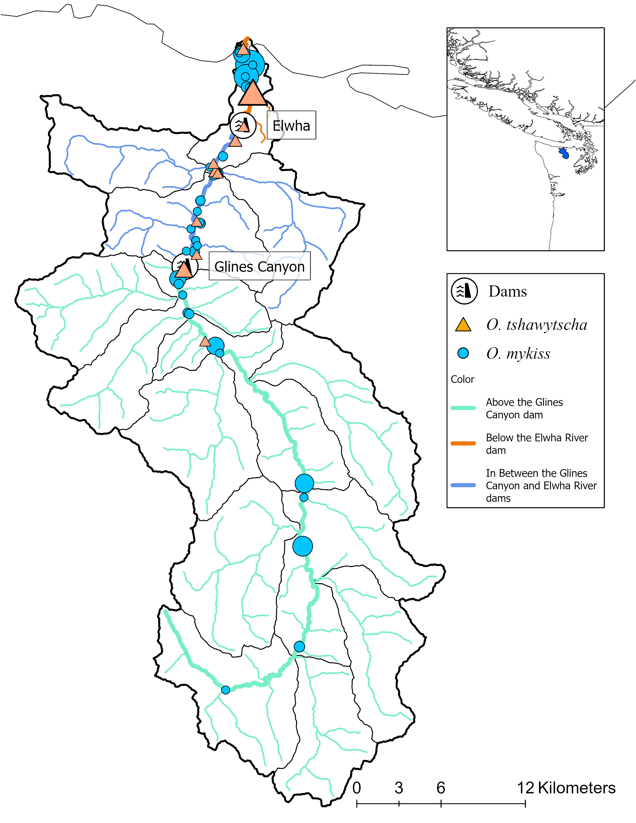
Figure 1 Study sites within the Elwha River basin as well as the location of the two dams removed in 2015. Each point represents a distinct sampling site for either O. mykiss (circles) or O. tshawytscha (triangles) within a broader sampling location (represented by color of the water and the relative dam location) along the Elwha River. Size of shape represents relative sample size.
We sampled O. tshawytscha tissue from post-spawn adult carcasses found along the river margins and banks. We assigned O. tshawytscha sampling locations based on the downstream GPS coordinate of the reach from which a carcass was collected. Though these sites did not necessarily represent the precise spawning location, they were likely geographically proximate at the reach scale (approximately 100 m–2 km). Since we sampled adult O. tshawytscha as carcasses, the return-timing of individual fish was unknown. All fish were sampled in 2014 or after, when the upper Elwha River Dam removal was underway. Thus, we considered all O. tshawytscha samples post-dam removal. However, to test if there were significant genetic differences between fish hatched pre and post-dam removal, we performed a supplementary set of analyses also assigned fish to age classes using scale ages (Appendix Materials and Methods). Samples taken from known hatchery-origin O. tshawytscha, identified by the presence of hatchery marks including otolith thermal marks, adipose clips, and coded wire tags (CWT), were included in this study. The O. tshawytscha hatchery broodstock are a native lineage broodstock program developed from fish caught in the Elwha; hatchery managers intentionally avoided releasing non-local stocks (Brannon and Hershberger, 1984). Both hatchery-origin and natural-origin fish were used for hatchery spawning, but it was not possible to target either origin for preferential spawning because most fish were not externally marked; hence hatchery-origin fish were not readily identifiable at spawning.
We sampled tissue from adult resident rainbow trout, adult Steelhead of both return migration times (early and late), outmigrating smolts (herein included in counts for Steelhead) and juvenile O. mykiss of unknown life-history forms across the watershed, prior to and post-dam removal, from fish returning from January through October (Table S1). We sampled juvenile O. mykiss using both backpack electrofishing and smolt traps (Pess et al, In Review). We designated trout fry as unknown life-history phenotypes unless recaptured as an adult or defined as a smolt (Fraik et al., 2021). We sampled hatchery-origin Steelhead samples from the Lower Elwha Klallam Tribe’s hatchery program, which was founded from native lineage broodstock developed from eyed eggs from naturally spawned adult O. mykiss sampled downstream of Elwha River dam from 2005–2011 (LEKT, 2012; Winans et al., 2016; Fraik et al., 2021). Hatchery-origin samples were included in this study. We collected natural-origin, adult O. mykiss via hook and line sampling and in steam netting (Denton et al., 2022b). We distinguished adult Steelhead from adult rainbow trout primarily based on body coloration and a size threshold (Steelhead fork length > 500 mm, rainbow trout fork length < 500 mm). Adult Steelhead were sampled in the main-stem Elwha River while migrating to their spawning sites or emigrating back to the sea after spawning. Thus, for O. mykiss, sampling location may not necessarily represent their exact spawning location. We assigned fish as pre-dam removal if they were sampled before 2013 and post-dam removal if they were sampled 2013 and beyond (Table S1). As scale ages were not available for O. mykiss, we could not assign O. mykiss to fish hatched pre and post-dam removal.
2.3 DNA sequencing, genotyping, and quality control
In total, 380 O. tshawytscha and 1,741 O. mykiss were sampled and prepared for Genotyping-in-Thousands by sequencing (GTseq). Sequence data for O. tshawytscha was obtained from McKinney et al. (In Prep), NCBI Bioproject PRJNA1020840, and reanalyzed for this study. DNA was extracted from O. tshawytscha and O. mykiss tissue punches stored on Whatman paper using the Promega Wizard SV genomic DNA extraction kit. All GTseq libraries were constructed separately for each species following the methods in Campbell et al. (2015). The O. tshawytscha GTseq panel contains 332 loci, 298 of which are putatively neutral and commonly used for population genetic studies, one sex identification marker, and 33 markers associated with return-timing variation in GREB1L/ROCK1 region (Hess et al., 2016; Thompson et al., 2019; Koch and Narum, 2020; Thompson et al., 2020). Genotypes for both species were called using the custom scripts in the GTScore pipeline (McKinney et al., 2020, available at GitHub - gjmckinney/GTscore: Pipeline for GTseq genotyping and quality control). Oncorhynchus mykiss samples were genotyped with the GTseq panel developed by Campbell et al. (2015) that contains 367 SNPs, of which 241 are putatively neutral and commonly used for population genetic studies, one is for sex identification, three are for diagnosing cutthroat trout (O. clarkii) and 122 markers that are putatively adaptive, of which 13 are associated with return-timing variation (Collins et al., 2020). Across both data sets, loci were filtered to remove potential and known tetrasomic loci. Samples with a high likelihood of DNA contamination (contamination score > 90%) and pairs of samples with duplicate genotypes (> 80% genotypes identical between each pair of individuals) were filtered out. For O. mykiss, we also removed individuals that had at least one cutthroat trout allele at one of the three species diagnostic loci.
Subsequent filtering for each species was performed in R v4.1.2 (R Core Team, 2022) using the package “adegenet” (Jombart, 2008; Jombart and Ahmed, 2011) for all the remaining SNPs. Using the minorAllele function we identified and removed 18 monomorphic loci from the O. tshawytscha and zero loci from the O. mykiss dataset. Next, we removed loci that were missing > 0.3 data among genotyped individuals (zero loci were removed from O. tshawytscha and five loci from the O. mykiss dataset) and individuals missing > 0.4 genotype data across loci (zero O. tshawytscha and 102 O. mykiss individuals).
The filtered SNPs for each species were then divided into two data sets: loci putatively involved in migration return-timing and putatively neutral loci. Given the specificity of our study question, we considered loci located in GREB1L/ROCK1 regions to be involved in migration return-timing, and the other adaptive loci were classified into the neutral genetic matrix. This also prevented loci that were adaptive in one system from being erroneously classified as adaptive in the Elwha River populations due to the geographic range of previous genomic outlier tests. Loci found in/near GREB1L/ROCK1 and previously identified as candidates for migration return-timing life-history variants included 28 SNPs in the O. tshawytscha panel and 11 SNPs in the O. mykiss panel that passed missing data thresholds (Campbell et al., 2015; Hess et al., 2016). We applied a Hardy-Weinberg equilibrium test to all of the remaining neutral loci in each species’ panel to identify loci deviating from expectations of Hardy-Weinberg equilibrium (HWE) using hw.test function in the R package “pegas” (Paradis, 2010). We applied a strict Bonferroni adjustment (Dunn, 1961) for multiple tests to generate the final list of putatively neutral loci for downstream analysis.
2.4 Population genetic and structure analyses across species
To investigate changes to the population genetic structure of O. mykiss and O. tshawytscha, we performed Discriminant Analysis of Principal Components (DAPC) using “adegenet” in R. For these analyses, we conducted four independent DAPC analyses for O. mykiss and one for O. tshawytscha. In the first two DAPCs for O. mykiss, we used the set of putatively neutral loci as determined by the HWE test for pre and post-dam removal fish (303 SNPs). In the second two DAPCs for O. mykiss, we once again separated samples temporally, but only retained loci explicitly designated as neutral in the GTseq panel (212 SNPs). We ran DAPC analyses on each set of putatively neutral loci in O. mykiss to compare the neutral genetic structure between our filtered loci and those identified as neutral in the panel. There were no putatively adaptive loci outside of the return-timing loci in the O. tshawytscha GTseq panel, therefore we only conducted one DAPC for all post-dam removal fish (271 SNPs). The number of genetic clusters (K) used in the DAPC analyses was informed by returning successive K-means with an increasing number of clusters. We considered the optimal K based on the lowest Bayesian Information Criterion (BIC) or within 2 ΔBIC (Jombart et al., 2010).
To estimate changes in population genetic diversity over time and space, we divided these temporal sets by sampling location relative to the location of the former dams (AD, ID and BD). Next, we divided our genetic data sets temporally pre and post-dam removal for O. mykiss. We included temporal comparisons of population genetic structure and diversity analyses for O. tshawytscha using scale analysis assignments in the Appendix (Appendix Figures 1–2, Appendix Tables 1–2). We tested the observed heterozygosity (HO), the inbreeding coefficient (FIS), and fixation index (FST) using the R package “hierfstat” (Goudet, 2005). We bootstrapped FIS values 100 times using boot.ppfis() to generate the 95% confidence interval for FIS. We assessed the significance of FIS by determining if the 95% confidence interval overlapped 0 (Goudet, 2005). KING relatedness statistics were calculated with neutral loci using vcftools (Danecek et al., 2011) “–relateness2” option. We also performed a permutation test with 1000 iterations to test the significance of FST. The p-value of FST was calculated by looking at the proportion of the permuted values that were greater than or equal to the observed values. We also estimated changes in the effective number of breeders (Nb) using the software “NeEstimator” 2.1 (Do et al., 2014). Input files were generated by modifying the genind_to_genepop function of the R package “graph4lg” (Savary et al., 2021) to allow for both indels and SNPs as the alternative allele. We calculated Nb using a random mating model of Linkage Disequilibrium method with a critical value of 0.05. We determined the statistical significance of our estimates using 95% critical intervals derived from jackknife estimates of Nb.
2.5 Riverscape genetics modeling
We tested two types of riverscape genetic models - Isolation by Environment (IBE) and Isolation by Resistance (IBR) using post-dam removal individuals (Figure 2). IBE represents spatial genetic variation created by the interactions between organisms and environments “at sites” (Wang and Bradburd, 2014). If this is the case, the genetic distances are correlated with the environmental differences at sites as heterogeneous environments influence gene flow. On the other hand, IBR represents a positive relationship between genetic distances and resistance distances focused on the environment “between sites”. Based on circuit theory, IBR calculates resistance distances, or cost distances, across the geographic range from factors interfering with migration (McRae, 2006). As IBE and IBR models test associations of genetic variation with variables “at sites” where fishes stay and “between sites” where fishes travel, respectively, these two riverscape genetic models can complement each other in their capture of both site-specific and corridor-specific environmental heterogeneity. The null model, or hypothesis, to both the IBE and IBR hypotheses was Isolation by Distance (IBD). This served as our null hypothesis as the expected relationship is a decrease in relatedness with increasing distance (Rousset, 1997) and following with Tobler’s First Law of Geography that things closer in space are more similar. We also expected this to explain patterns of gene flow for return-timing genetic distance as we expect that early-return life-history forms evolved in part to exploit favorable environmental conditions coinciding with earlier arrival for fish that must migrate long distances. We quantified this in our IBD models as river kilometer (rKm) or distance from the mouth of the river (Benda et al., 2007) (Figure 2). If IBD represents the best model, genetic distance should be proportional with rKm (Selkoe et al., 2016). Alternative models and the environmental variables included in each model are listed in Table 1.
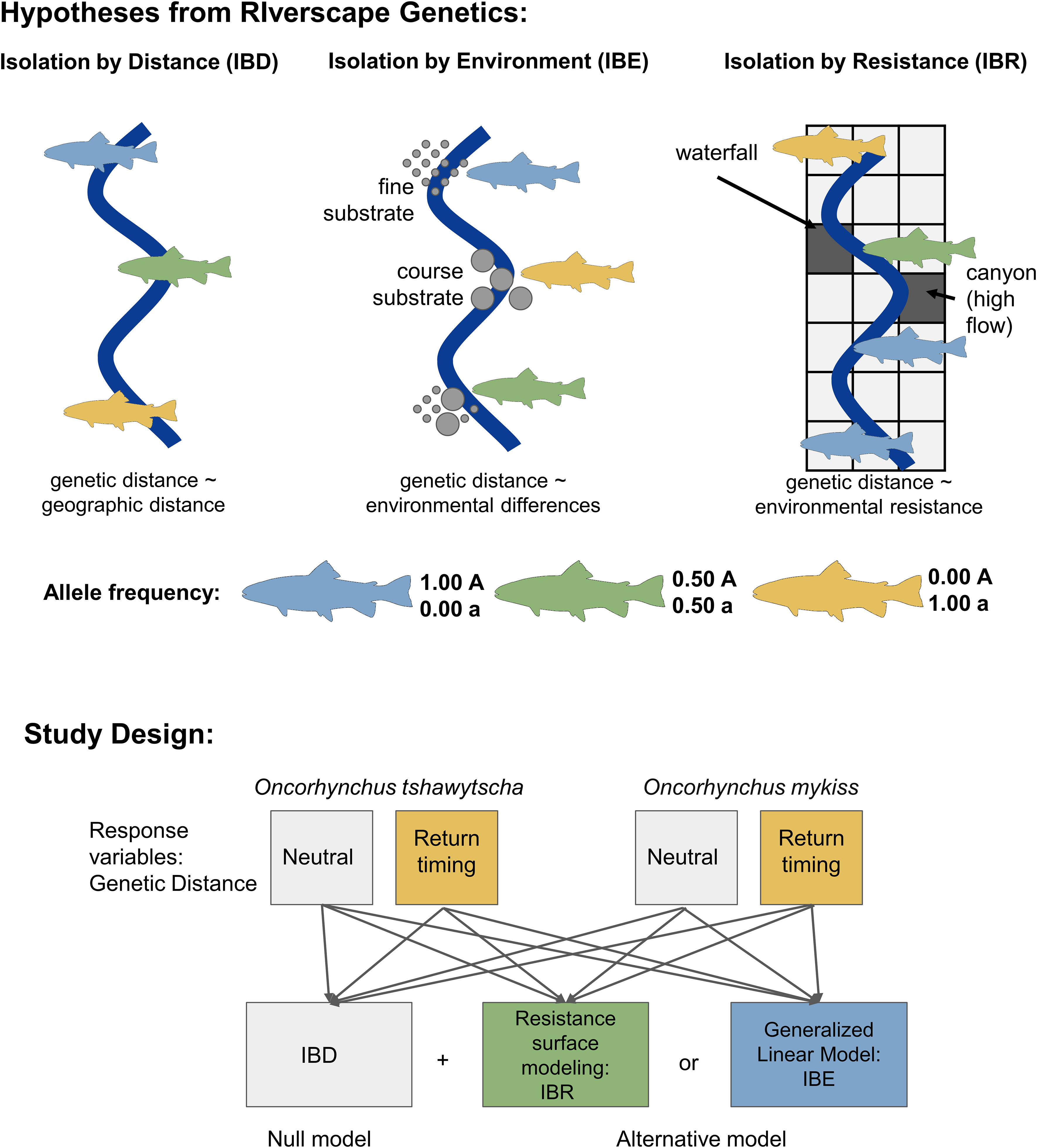
Figure 2 Schematic of the landscape genetics hypotheses tested in our study design. Isolation by distance (IBD) is a pattern of decreasing genetic similarity as geographic distance increases due to limitations in movement and gene flow. Isolation by environment (IBE) is a pattern where genetic similarity is influenced by the environment at a location instead of the geographic distance. Conversely, isolation by resistance (IBR) is a pattern of decreasing genetic similarity based on the landscape between two sites. Isolation by distance represents the null hypothesis to isolation by environment and isolation by resistance. In this study, the response variable for each model is neutral or return-timing genetic distance for each species.
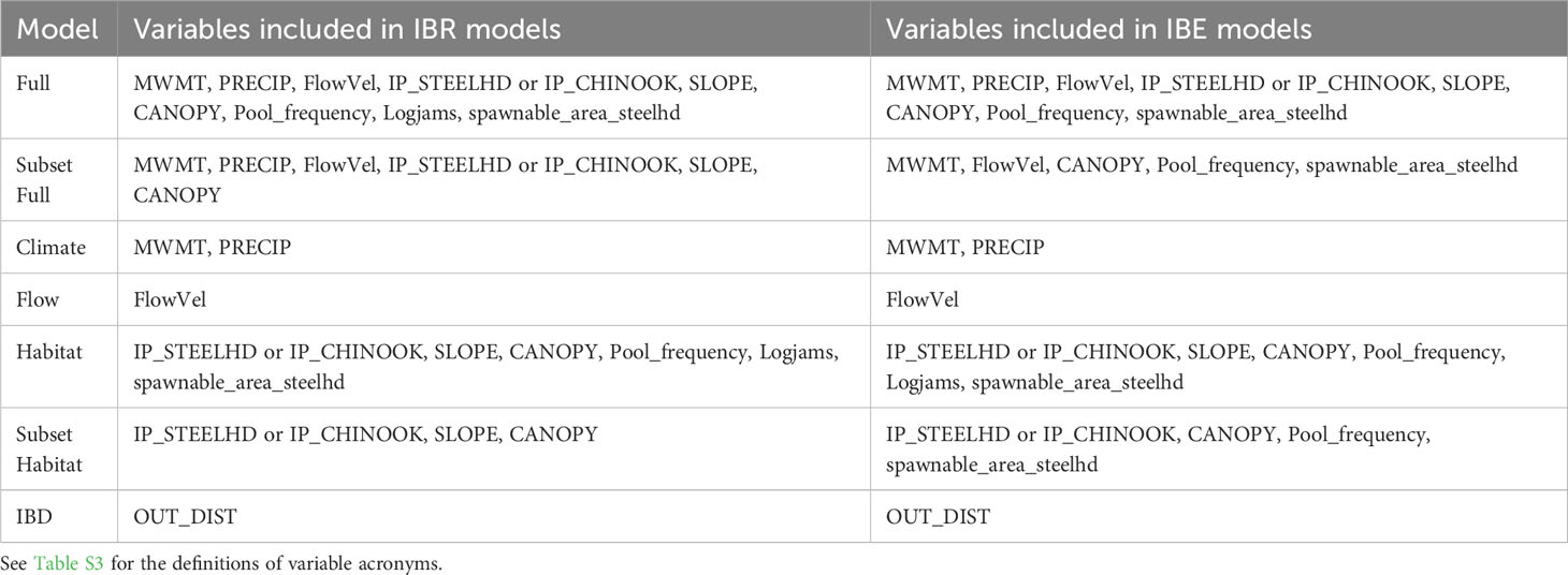
Table 1 Environmental variables included for each isolation by environment (IBE) and isolation by resistance (IBR) riverscape genetics model tested.
2.5.1 Genetic distance matrix generation for landscape genetics models
We generated two sets of neutral and return-timing genetic distance matrices for each species: one for IBE models and one for IBR models. We tested neutral and return-timing genetic distances separately to examine how riverscape variables may affect both neutral and return-timing genetic variation. For IBE models we calculated neutral genetic distance using the loading scores of the first principal component from the DAPC analysis that characterized the underlying genetic structure of post-dam removal individuals. The proportion of early return-timing alleles in each individual was used to generate the return-timing genetic distance matrices. For IBR models, both neutral and return-timing genetic distances were calculated among every sampling site as Roger’s/Classical Euclidean distance (Rogers, 1972; Avise, 1994) using the dist.genpop function of the R package “adegenet” with the method argument set to 4 (Jombart, 2008). We also calculated Nei’s distance (method = 1) (Nei, 1972; Nei, 1978; Avise, 1994) but only used Roger’s/Classical Euclidean genetic distance for downstream analyses due to the high correlation between them (r > 0.97).
Given that O. tshawytscha were only sampled as adults and O. mykiss were sampled as adults, juveniles and unknown life-history forms, we tested one O. tshawytscha dataset and three O. mykiss datasets: all O. mykiss, adult Steelhead, and juvenile O. mykiss.
2.5.2 Isolation by environment modeling: at-site characteristics
To test if environmental differences at spawning sites influence genetic variation in our study species, we centered and scaled the uncorrelated environmental variables describing the stream temperature, flow, habitat, and riverbed substrate at our sampling sites where individuals were sampled post-dam removal. We subset our environmental variables into five models: (1) null, including only river kilometer, (2) climate, including MWMT (maximum weekly maximum temperature) and precipitation, (3) flow, including flow velocity, (4) habitat, including canopy cover, slope, intrinsic habitat potential, pool frequency, number of logjams per 100m, and amount of spawnable habitat, and (5) full, including all variables except river kilometer (Table 1). For all five models, we rechecked for multicollinearity using variance inflation factor (VIF) (Naimi et al., 2014) and removed the variable with the greatest VIF until all remaining variables had a VIF of less than 5. The resulting model subsets are described in Table 1. We used linear models for neutral response variables and generalized linear models with a binomial distribution for return-timing response variables due to their bimodal distribution using the “stats” in R package (R Core Team, 2022). Model residuals were visually inspected for model assumptions. We compared each suite of IBE models using Akaike information criterion (AIC) (Burnham and Anderson, 2002).
2.5.3 Isolation by resistance modeling: between-site characteristics
To test if environmental characteristics between spawning sites influence genetic variation in our study species, we fit IBR models to our data. These included: (1) null model/IBD where distance and not environment drives patterns of genetic distance, represented by river kilometers between sites, (2) climate model, including MWMT (maximum weekly maximum temperature) and precipitation, (3) flow model, including flow velocity, (4) habitat model, including canopy cover, slope, intrinsic habitat potential, pool frequency, number of logjams per 100m, and amount of spawnable habitat, (5) subset of the habitat model, including canopy cover, slope, and intrinsic habitat potential, excluding pool frequency, number of logjams per 100m, and amount of spawnable habitat which had a narrow range of cells, (6) full model, including all variables except river kilometer, (7) subset of the full model, including all variables except river kilometer, pool frequency, number of logjams per 100m, and amount of spawnable habitat (Table 1).
We used the R package “ResistanceGA” (Peterman, 2018) for modeling which uses a machine learning algorithm inspired by the process of natural selection genetic algorithm (Forrest, 1993), and maximum likelihood population effects regression (MLPE) that accounts for non-independence of data from the same populations (Clarke et al., 2002) in resistance surface optimization. Variables identified as uncorrelated were cropped to the Elwha river region and reprojected to the same geo-reference system (NAD83) of Elwha template raster derived from the NorWeST’s Washington Coast shapefile (Isaak et al., 2017) using the R package “terra”(Hijmans, 2022). Shapefiles were rasterized to a SpatRaster with a resolution of 0.001 degree. We then converted to RasterLayer and RasterStack using the R package “raster” (Hijmans, 2023), which is required by ResistanceGA. The “NA’’ values in each raster layers were set to 10 * maximum value of the layer for resistance surface computation due to the requirements of the ResistantGA algorithms.
We applied the “commuteDistance” option and “log-likelihood” as the objective function in ResistanceGA to optimize the effective resistance distance and resistance surface. Bootstrapping with 1,000 iterations was conducted to compare among successfully optimized models and choose the most likely one. IBR models with juvenile O. mykiss genetic distances were compared without bootstrapping due to an insufficient number of populations in the subsequent MLPE step. Models with each genetic distance were compared based on AIC calculated within ResistanceGA and optimal models with ΔAIC less than 2 were presented for each genetic distance.
3 Results
3.1 Genotype filtering to generate neutral and return-timing genetic datasets
After filtering, we retained a total of 278 SNPs and 354 O. tshawytscha individuals and 314 SNPs and 1,363 O. mykiss individuals (Supplementary Table S1). Of those filtered loci, 28 SNPs from the O. tshawytscha panel and 11 SNPs from the O. mykiss panel found in or near the GREB1L and ROCK1 genes, previously identified as candidates for migration return-timing life-history variants, were retained (Campbell et al., 2015; Hess et al., 2016). We ultimately removed one O. tshawytscha SNP (Bonferroni adjusted p-value < 0.00015) and 12 O. mykiss SNPs (Bonferroni adjusted p-value < 0.00015) that were out of HWE for downstream population and riverscape genetic analyses. Ultimately, this allowed us to retain 250 and 303 putatively neutral O. tshawytscha and O. mykiss SNPs.
3.2 Neutral genetic structure across species and space
Based on BIC, our population genetic structure analysis supported different numbers of genetic clusters or populations between species over time (Figure 3, Figures S1, S2, Appendix Figures 1–2). For O. tshawytscha, we identified one cluster post-dam removal (Figure 3C, Figure S1E) and no pairwise FST values between any pair of populations were significant (Table S2). Pre-dam removal DAPC analysis supported four to six clusters of O. mykiss pre-dam removal (Figures S1A, C) that we visualized as five clusters (Figures 3A, B). Post-dam removal, however, we detected five to ten clusters amongst our O. mykiss samples (Figures S1B, D). Pairwise spatial and temporal estimates of FST in O. mykiss supported significant, but small, changes in genetic structure across both space and time. We observed few differences in patterns of genetic diversity among species when looking at each time period or sampling location (Table 2). For O. tshawytscha, we observed no evidence of significant inbreeding across sampling locations as measured by FIS statistics with 95% confidence interval overlapping zero, when considering individuals from all sampling locations. For O. mykiss, we observed small positive FIS statistics with 95% confidence intervals significantly greater than zero, when considering individuals from all sampling locations, below dam only, and in-between dam only. There were no changes in the direction or significance of the FIS statistic over time or space in O. mykiss. We observed no significant relatedness, as measured by the KING statistic, in either O. tshawytscha or O. mykiss when samples were grouped by space and time.
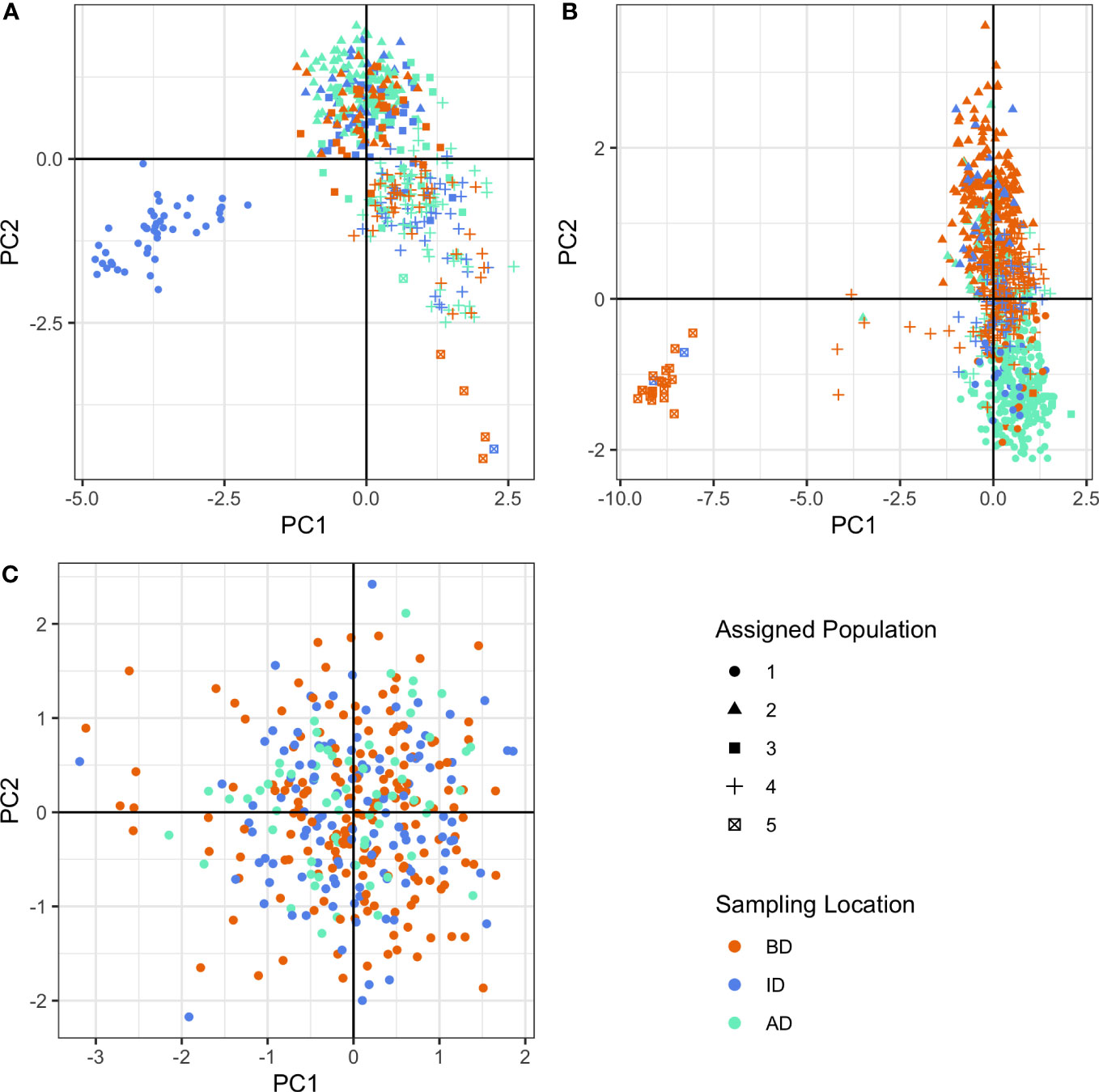
Figure 3 Discriminant analysis of principal components (DAPC) clusters using neutral loci for (A) O. mykiss pre-dam removal, (B) O. mykiss post-dam removal, and (C) O. tshawytscha post-dam removal. Colors represent sampling locations (BD: Below the Elwha River Dam, ID: In between the Elwha River and Glines Canyon Dams, AD: Above the Glines Canyon Dam). Shapes represent assigned populations.
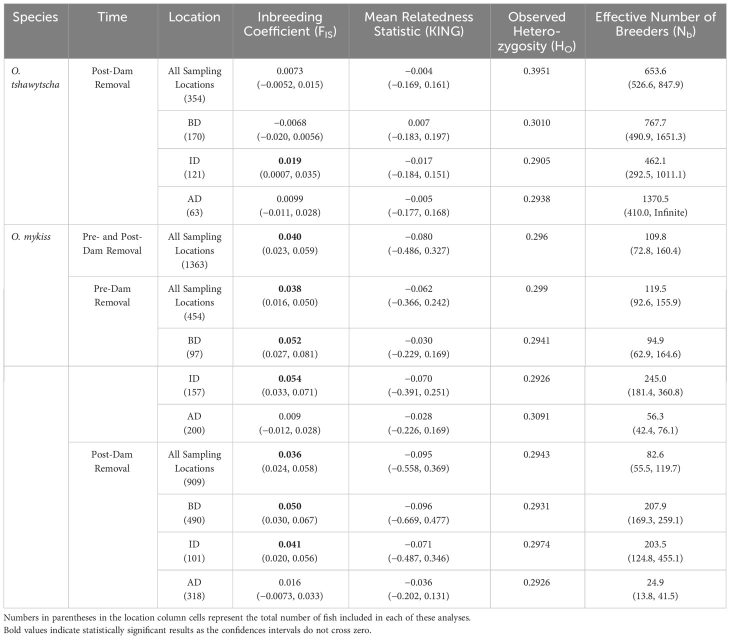
Table 2 Summary of relative levels of inbreeding (FIS, 95% confidence intervals in brackets with the bold significant results), mean relatedness statistic (KING, 95% confidence intervals in brackets), population genetic diversity (HO), and effective population size (Nb, 95% confidence intervals in brackets) for both salmonid species O. tshawytscha and O. mykiss pre and post-dam removal above dams (AD), in between the dams (ID) and below the dams (BD).
For O. tshawytscha, sampling location had no association with genetic clustering (Figure 3C). There was also no association of sampling location with O. tshawytscha genetic clustering when O. tshawytscha samples were classified as individuals hatched pre-dam removal or post-dam removal (Appendix Figures 1–2). For O. mykiss, some individuals collected from ID were highly discriminated from other sampling locations pre-dam removal (Figure 3A), while some individuals collected from BD were highly discriminated from other sampling locations post-dam removal (Figure 3B). For O. mykiss, genetic clusters tended to differentiate individuals collected BD from individuals collected AD post-dam removal along the second principal component axis (Figure 3B). We identified similar genetic clustering restricting our DAPC analyses to the 212 loci classified as neutral in the O. mykiss panel (Figure S2).
3.3 Three return-timing haplotypes were detected in both species
On average, single nucleotide polymorphisms (SNPs) in and near the GREB1L/ROCK1 genes genotyped using the GTseq panel were in linkage disequilibrium and phased into haplotypes (O. tshawytscha r2 = 0.48; O.mykiss r2 = 0.50). We identified three distinct haplotypes in each species post-dam removal: late return-timing (Fa, Win), early return-timing (Sp, Su) and recombinant haplotypes (FaR, WinR) for O. tshawytscha and O. mykiss (Figures 4, 5).

Figure 4 (A) Three haplotypes are detected post-dam removal in O. tshawytscha. Each column of the heat map represents one of the 29, putatively adaptive return-timing loci with each color of the heat map representing the early return-timing alleles or late return-timing allele. Each row represents one individual, with the dendrogram on the x-axis showing the most parsimonious clustering of individuals based on the haplotypes phased from the early return-timing loci. The vertical bar represents the haplotype called for each individual with haplotypes primarily containing early return-timing alleles, late return-timing alleles and a combination of the two. (B) The proportion of the three haplotypes in O. tshawytscha sampled below (BD), in-between (ID) and above (AD) the former dams post-dam removal. The numbers represent the sample size for each haplotype. (Fa: Fall, FaR: Fall Recombinant, Sp: Spring).
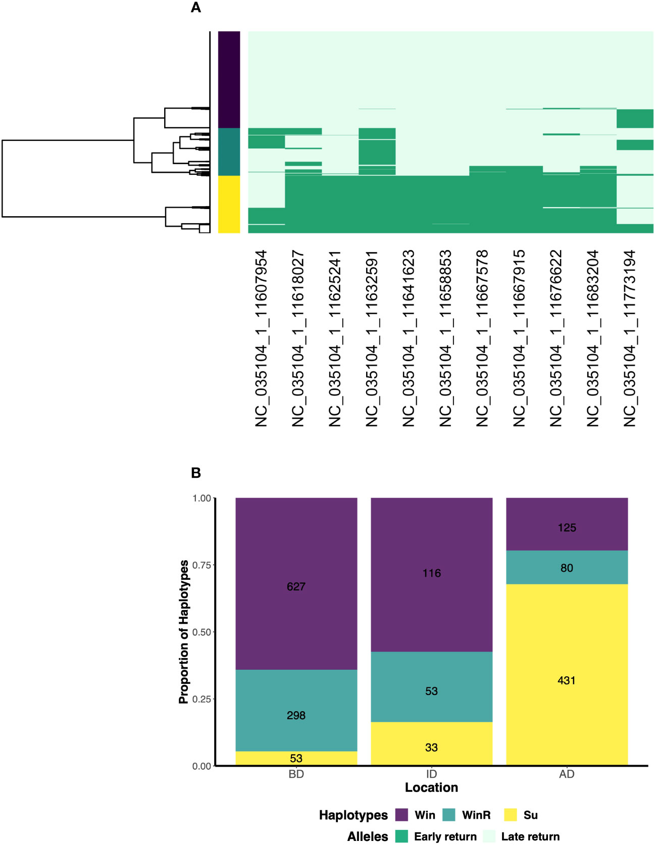
Figure 5 (A) Three haplotypes are detected post-dam removal in O. mykiss. Each column of the heat map represents one of the 11, putatively adaptive return-timing loci with each color of the heat map representing the early return-timing alleles (dark green) or late return-timing allele (light-green). Each row represents one individual, with the dendrogram on the x-axis shows the most parsimonious clustering of individuals based on the haplotypes phased from the early return-timing loci. The vertical bar represents the haplotype called for each individual with the yellow haplotype containing primarily early return-timing alleles, the purple primarily late return timing alleles and the green appears to be a combination of the two. (B) The proportion of the three haplotypes in O. mykiss sampled below (BD) in-between (ID) and above (AD) the former dam populations post-dam removal. The numbers represent the number of individuals containing each haplotype. (Win: winter, WinR: Winter Recombinant, Su: Summer).
For O. tshawytscha, recombinant haplotypes were the most common (FaR.) (N = 410), followed by late return-timing (Fa) (N = 175) and then early return-timing (Sp) (N = 123) haplotypes (Figure 4B). Early return-timing (Sp) haplotypes had 85.7% early return-timing alleles on average (range = 0.71–1.00, σ = 0.008), while recombinant (FaR: μ = 0.158, range = 0.07–0.35, σ = 0.0011) and late return-timing haplotypes (Fa: μ = 0.08, range = 0.036–0.14, σ = 0.0013) had substantially fewer alleles on average. For O. tshawytscha, this included mostly recombinant haplotypes (FaR) (N = 198), followed by late return-timing (Fa) (N = 75), and then early return-timing (Sp) (N = 55) haplotypes (Figure 4). Fish hatched pre-dam removal mostly had mostly recombinant O. tshawytscha haplotypes (FaR) composed of 15.0% early return-timing alleles on average (Appendix Figure 3).
For O. mykiss, late return-timing haplotypes were also the most frequently detected post-dam removal (Win) haplotypes (N = 868), followed by early return-timing (Su) haplotypes (N = 517) and then recombinant (WinR) (N = 431) haplotypes (Figure 5B). The early return-timing (Su) haplotypes were composed of 86.8% early return-timing alleles on average (range = 0.64–1.00, σ = 0.005), while recombinant (WinR: range = 0.09–0.73, σ = 0.002) and late return-timing haplotypes (Win: range = 0–0.36, σ = 0.002) were composed of 25% and 2.1% early return-timing alleles on average respectively.
We did not detect any significant differences in the frequency of early return-timing alleles among O. tshawytscha spatially post-dam removal (Figure 6A) or over time (Appendix Figure 4). However, we identified a number of statistically significant pairwise comparisons of early return-timing allele frequencies across O. mykiss, sampled from different parts of the river over time (Figure 6B). Pre-dam removal, we found that BD fish (μAF = 0.15) had significantly lower early return-timing allele frequencies compared to AD (μAF = 0.26; Wilcox test, Bonferroni adjusted p-value = 0.002), but not ID fish (μAF = 0.16; Wilcox test, Bonferroni adjusted p-value = 0.006). Post-dam removal, we observed statistically significant differences in the allele frequencies observed across all geographic pairwise comparisons (Wilcox test, Bonferroni adjusted p-value < 0.05). We found that fish sampled AD (μAF = 0.608) had significantly higher frequencies of early return-timing alleles than those sampled BD (μAF = 0.108; Wilcox test, Bonferroni adjusted p-value = 9.24e-71) and ID (μAF = 0.207); ID fish had significantly higher early return-timing alleles than BD (Wilcox test, Bonferroni adjusted p-value = 0.021). Early return-timing alleles were more frequent in fish sampled AD post-dam removal (μAF = 0.608) than those sampled pre-dam removal (Wilcox test, Bonferroni adjusted p-value = 7.21e-25). We detected the highest proportions of both early return-timing haplotypes and genotypes in adult Steelhead sampled AD post-dam removal between July and October (Figure S3).
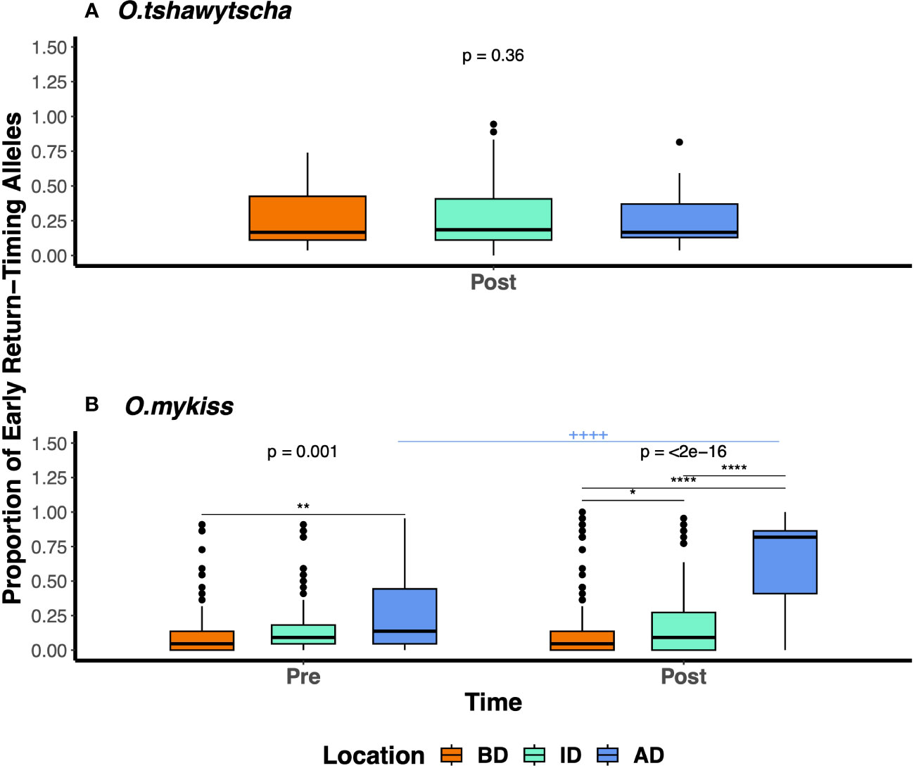
Figure 6 The proportions of early return-timing alleles in GREB1L in (A) O. tshawytscha and (B) O.mykiss post-dam removal below (BD), in-between (ID), and above (AD) the dam. The Bonferroni adjusted p-values generated by Kruskal test across three locations were labeled above each time period. The asterisk (*) represents statistically significant pairwise comparisons with the Bonferroni adjusted p-values reported across sampling locations within the same time period. The plus (+) represents statistically significant pairwise comparisons with the Bonferroni adjusted p-value reported among fish sampled from the same sampling locations, across time (cutpoint for p-values: */+=0.05, **/++=0.01, ****/++++=0.0001).
3.4 Reduced environmental dataset retained for riverscape genetics models
We ultimately retained 11 out of the 26 environmental variables after testing for correlations for use in our riverscape genetic models for both O. tshawytscha and O. mykiss (Table S3, Figures S4–S6). These included stream temperature (Maximum Weekly Maximum Temperature between 2015–2017; MWMT), flow velocity, habitat intrinsic potential for O. tshawytscha, habitat intrinsic potential for Steelhead, slope, riparian canopy, pool frequency, logjams per 100 m and spawnable habitat (Table 1, Table S3, Figure S7). This subset represented summarized measures of dynamic variables (i.e., stream temperature), predicted metrics based on geometry (i.e., flow velocity), and single measures of relatively static variables (i.e., slope and canopy) that change on the scale of years to decades.
3.5 IBD as a strong explanatory variable across IBE and IBR models
3.5.1 IBE indicates at-site environment and IBD influence genetic differentiation
Isolation by Environment (IBE) models identified at-site environmental variables associated with neutral and return-timing genetic differentiation in O. mykiss individuals sampled post-dam removal. For O. tshawytscha, while no individual environmental variable was statistically significant, the IBD model, followed by the climate and flow models, had the lowest AICs to explain neutral, at-site, genetic differentiation. The habitat and full models had the lowest AICs to explain return-timing genetic differentiation for O. tshawytscha, also with no statistically significant individual environmental variable (Table 3). When combining all O. mykiss life-stages in one model, the IBD model had the lowest AIC to explain neutral and return-timing genetic differentiation (Table 3). For just adult Steelhead, the habitat and full models had the lowest AIC to explain neutral genetic differentiation, while the IBD, the habitat model, and full model equally explained return-timing genetic differentiation (Table 3). Within these top models for return-timing genetic variation, river kilometer and pool frequency both had significant positive relationships with the proportion of early return-timing alleles. For juvenile O. mykiss, the habitat and full models equally explained both neutral and return-timing genetic differentiation (Table 3). Within these full models, canopy cover and intrinsic habitat potential had significant positive and negative relationships respectively with the proportion of early return-timing alleles (Table 3, Supplementary Data File 1).
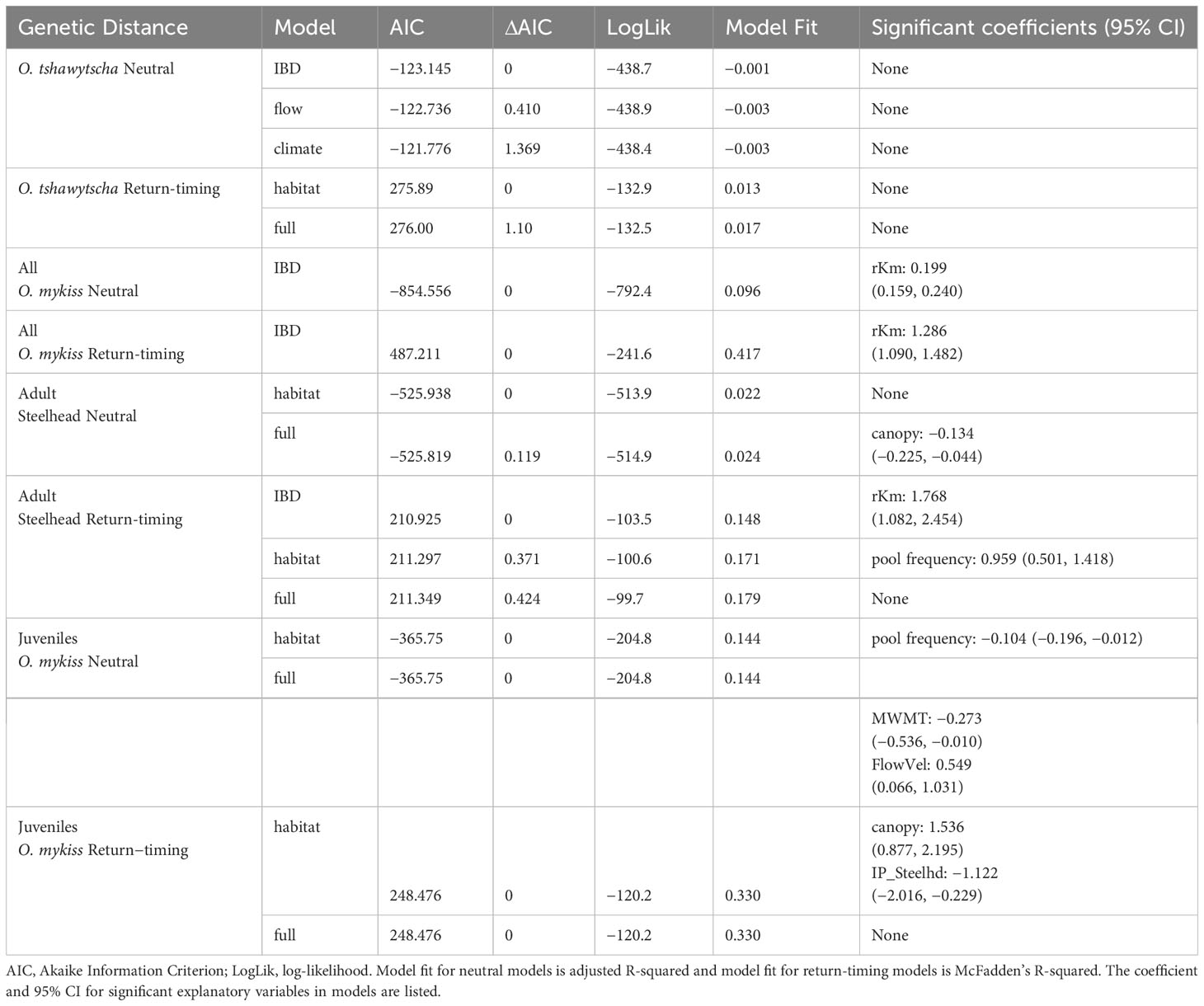
Table 3 IBE model results representing the influence of environmental variables on neutral and return-timing genetic variation.
3.5.2 IBR modeling indicates IBD best explains genetic variation
We tested four IBR models for O. tshawytscha and twelve IBR models for O. mykiss, similar to IBE models to account for differences in the life-history stage and methods of sampling included for each species (Figure 2, Table 4). Across both species and both genetic distance types, IBD was the best model for all the cases of IBR modeling conducted (Figure 7, Table 4, Supplementary Data File 2). The optimized resistance surface even displayed the same value of “1” all over the extent in some cases (Figures 7A, B, H), which indicated that genetic distances could not be explained better than the Euclidean geographic distances (Table 4). Second and third optimal models (ΔAIC < 2) were identified for several cases, including all O. mykiss neutral (flow model), all O. mykiss return-timing (flow and climate model), adult Steelhead neutral (flow model), and juvenile O. mykiss return-timing (flow model) genetic distances (Figure S8).
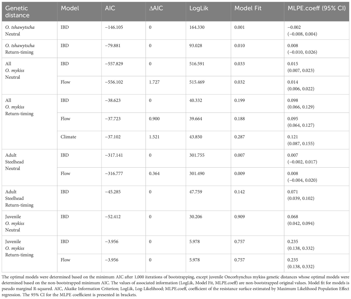
Table 4 IBR model results representing the influence of environmental variables on neutral and return-timing genetic variation.
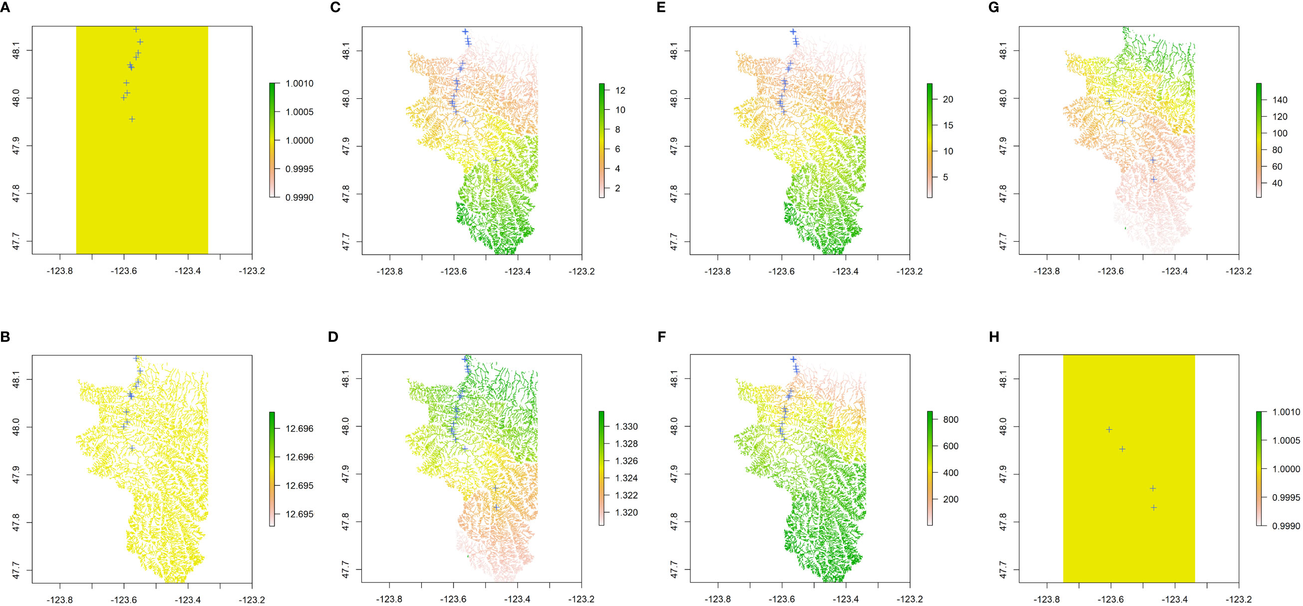
Figure 7 The best optimal resistance surfaces by ResistanceGA for each response matrix of (A) O. tshawytscha neutral, (B) O. tshawytscha return-timing, (C) all O. mykiss neutral, (D) all O. mykiss return-timing, (E) adult Steelhead neutral, (F) adult Steelhead return-timing, (G) juvenile O. mykiss neutral, (H) juvenile O. mykiss return-timing genetic distance. Green colors represent higher resistance values while yellow to red represent lower resistance values. Optimized resistance values for (A, H) were homogeneous across the geographic extent, implying their genetic distances could not be explained by environmental variables, any better than euclidean-distance-based Isolation by Distance.
4 Discussion
In this study, we leveraged the removal of two large dams on the Elwha River to understand how habitat restoration impacted the return and reestablishment of distinct ocean migrating life-history forms of O. tshawytscha and O. mykiss to their historical distribution. While we observed no difference in the proportion of early return-timing alleles in O. tshawytscha across the watershed, we observed significant differences for O. mykiss across the watershed for samples collected both pre- and post-dam removal. Specifically, the proportion of early return-timing alleles was greater in O. mykiss sampled above dam locations than below dam locations. Using riverscape genetics analyses, we found that return-timing genetic variation was more strongly influenced by environmental differences compared to neutral variation. By exploring the relationships of at- and between-site environmental characteristics, we identified significant patterns of spatial genetic variation in O. mykiss. For both species, the patterns and processes are still actively shifting in response to these restoration efforts; however, we show here early evidence of the importance of considering adaptive potential of ocean return-timing and neutral genetic variation in understanding species responses to restoration efforts.
Lack of population genetic structure and decreases in genetic diversity observed in O. mykiss may be, in part, an artifact of the study design. Previous work documenting Elwha River O. mykiss using microsatellite and tens of thousands of SNP loci found that both dams and anadromous barriers generated significant genetic structure pre-dam removal (Winans et al., 2016). Post-dam removal, structure appeared to decrease as gene flow resumed between formerly allopatric populations (Fraik et al., 2021). While we know the natural-origin Steelhead populations in the upper river have significantly increased post-dam removal (Denton et al., 2022b; Peters et al., 2022; Pess et al., In Review). We observed diminished Nb above the former dams, but an increase below the former dams. Biologically, this might reflect down river movements of resident rainbow trout after dam removal and greater overall admixture. Alternatively, this could be an artifact of sampling location and design since Steelhead may not have been sampled at spawning sites. Ascertainment bias in the genotyping panels utilized for this study could also explain deviations from previous work. One half of the neutral loci in the O. mykiss GTseq panel (92 SNPs) were selected to delineate genetic stocks at a river basin or watershed level, across reporting groups in the Columbia River and across the US West Coast (Narum et al., 2010; Abadía-Cardoso et al., 2011; Limborg et al., 2012). Given the geographic focus of our study is considerably smaller than the target spatial scale of the panels, we may be observing higher genetic covariance amongst the SNP genotypes of fish from the Elwha River watershed, in line with the intended purpose of the panel.
Similar to O. mykiss, we did not observe significant evidence of genetic structure in O. tshawytscha. The reestablishing O. tshawytscha in the Elwha are heavily dominated by hatchery spawners that were generated from the small, natural-origin population that remained below the dams decades after dam removal (McHenry et al., 2022). We have evidence that eleven of the O. tshawytscha sampled in the Elwha River might represent strays (McKinney et al., In Prep) and may encompass greater genetic diversity. As the neutral loci in the O. tshawytscha panel were designed to delineate genetic stocks, we may be capturing the introduction of straying fish admixing with Elwha River endemic O. tshawytscha. While there is limited data to determine how genetic diversity and structure changed over time (Appendix Table 2), these genotypes provide an important baseline for O. tshawytscha as limited genetic studies have been published on Elwha and surrounding Puget Sound populations to date (McKinney et al., In Prep; Ruckelshaus et al., 2006; Winans et al., 2008).
While we did not find evidence of significant neutral genetic structure between locations, there were significant deviations in the return-timing allele frequencies across the watershed in O. mykiss, but not O. tshawytscha (Figure 6). In O. mykiss, there were higher frequencies of the early return-timing haplotypes and alleles in fish sampled above the former dams compared to below the dams post-dam removal (Figures 5, 6). In the Elwha River, both early return-timing life-history forms of each species were extirpated following dam construction (DOI, 1996). The resident form of O. mykiss, rainbow trout, was able to persist in the middle and upper watershed, while O. tshawytscha and the anadromous form of O. mykiss, Steelhead, were limited to seven river kilometers of spawning habitat below the dams (McHenry et al., 2017). While Steelhead were not able to return to spawn above the dams, these land-locked O. mykiss harbored high proportions of the early return-timing alleles and maintained high levels of standing genetic variation river-wide (Hiss and Wunderlich, 1994; Winans et al., 2016; Fraik et al., 2021; Fraik et al., 2022). Steelhead reestablished in the upper river before O. tshawytscha (Duda et al., 2020; Duda et al., 2021), with the first early return-timing Steelhead detected in 2013 (Personal Comm. J. McMillan) and Chinook detected in 2022 (Personal Comm. R. Peters). A high proportion of these summer Steelhead ascending the former dammed river have been shown to be descendants of the land-locked, above-dam ancestries (Fraik et al., 2022). The preference for summer Steelhead to spawn in colder, snow-melt fed water (Busby et al., 1996) may also suggest there is pleiotropy at the return-timing genetic locus for local adaptation (Micheletti et al., 2018).
Riverscape genetic models indicated that patterns of return-timing variation in O. mykiss were affected by sampling site environmental differences. Variation in frequencies of early return-timing alleles in adult Steelhead and juvenile O. mykiss at sampling sites were best explained by habitat and full models. Pool frequency was a significant covariate in the habitat model for adult Steelhead, suggesting that spawning Steelhead adults with different early return-timing genotypes may be differentially impacted by spawning ground habitat characteristics. Similarly, juvenile O. mykiss return-timing, as well as neutral genetic variation, was best explained by habitat variables (pool frequency and canopy) across rearing habitat. When considering all O. mykiss cumulatively, the significance of these models diminished. Consistent influence of habitat characteristics across age classes and genetic response variables suggests that these covariates may be biologically significant, reflecting age class specific responses.
Broadly, we found that geographic distance best explained patterns of neutral gene flow both at-site (IBE) and between-site (IBR) for most species’ models. The full and habitat IBE models were the optimal neutral models for Steelhead and juvenile O. mykiss, but not for O. tshawytscha. The lack of environmental influence observed in the O. tshawytscha models most likely reflects the limited, or lack of, environmental heterogeneity among O. tshawytscha sampling sites. While water temperature is usually a significant environmental factor influencing growth, migration and movement in salmonids (Brewitt and Danner, 2014; Kendall et al., 2015; Armstrong et al., 2021; Pitman et al., 2021), temperature variation throughout the Elwha is not physiologically limiting (Myrick and Cech, 2005; Siegel et al., 2022; Siegel et al., 2023) and probably not impacting gene flow. Alternatively, these differences could be the by-product of how O. mykiss were sampled at specific sampling sites at known age classes compared to O. tshawytscha, which were sampled across river reaches post-spawning. For example, MWMT stream temperature standard deviation for O. mykiss was 0.44 Celsius (n = 19, mean = 16.1 Celsius, range = 15.1–16.5 Celsius) and O. tshawytscha was 0.37 Celsius (n = 9, mean = 16.6 Celsius, range = 16.3–17.4 Celsius), reflecting a narrow range of environmental variation across the sampling locations. However, these differences in stream temperature could also reflect the statistical uncertainty around the derivation of environmental point estimates from stream reaches rather than geographic points. Regardless, we may simply lack the statistical power to detect the influence of the environment on neutral variation due to a more homogenous resistance surface.
In this study, we explicitly did not conduct any direct comparisons between O. tshawytscha and O. mykiss because of several important differences in the founding populations, sampling methods, and stage of recovery of the two species in the Elwha River. First, the founding Elwha O. tshawytscha is not only smaller than the O. mykiss population but represents lower return-timing genetic diversity compared to O. mykiss (Figures 4, 5). Both species populations are bolstered by hatchery programs that were founded from below dam, natural-origin Elwha broodstock that do not necessarily select for diversity at the GREB1L/ROCK1 locus. While these hatchery fish make up a large proportion of the reestablishing O. tshawytscha population, they make up less of the Steelhead population (Pess et al., In Review; Denton et al., 2022a; Denton et al., 2022b; McHenry et al., 2022; Peters et al., 2022). Reestablishing Steelhead possess ancestry from below dam, similar to those of hatchery fish, as well as formerly above and in-between dam ancestries that contain greater return-timing genetic variation (Fraik et al., 2021). Second, the temporal and spatial extent of sampling was more limited for O. tshawytscha than for O. mykiss. The relatively short time frame of sampling for O. tshawytscha and the majority of samples coming from the lower reaches of the Elwha is a direct result of this species being in an early stage of reestablishment in the Elwha River. While these sampling limitations do impede the power of temporal and spatial analyses for O. tshawytscha, our study was able to document contemporary patterns, or the lack thereof, of genetic variation in the study area. For example, while IBD models were the most optimal for O. tshawytscha, the coefficients were not significantly different from zero reflecting no clear association or return-timing variation with river kilometer. Thus, we may be observing an artifact of a founder effect generated by genetic stochasticity rather than IBD (Gaggiotti et al., 2004; Weigel et al., 2013). In contrast, we observed a positive association between geographic distance and return-timing genetic distance and resistance in O. mykiss, regardless of age class. These results may occur because distance can represent a proxy for the cumulative differences in environmental conditions experienced by each return-timing life-history as individuals move further upriver from the ocean (Rougemont et al., 2023), and our sampling sites for O. mykiss extended over twice the distance upstream compared to O. tshawytscha sampling sites.
Our study provided a framework for testing the impacts of a significant environmental change, large barrier removal, on the recovery of two important species and their key life-history forms. The reservoir of neutral and return-timing genetic variation maintained in resident rainbow trout above the dams appeared to allow for rapid, robust reestablishment of diverse O. mykiss life-history forms river wide post-dam removal. While we did not have phenotype data to characterize recovery of each life-history form in the watershed, we were able to infer how adaptive potential underlying these life-history forms is distributed (Hess et al., 2016; Prince et al., 2017; Micheletti et al., 2018; Narum et al., 2018; Thompson et al., 2019; Collins et al., 2020; Ford et al., 2020; Koch and Narum, 2020; McKinney, 2020; Willis et al., 2020; Willis et al., 2021; Tigano and Russello, 2022; Waples et al., 2022). We observed species and age-class specific patterns of genetic distances structured among sites that shows how at- and between-site environmental heterogeneity may influence O. mykiss. Given that O. tshawytscha were extirpated from the river above the former dams, we are still in the early stages of observing their reestablishment in the upper watershed. We were able to test biologically informative hypotheses about environmental heterogeneity that influence species, population and life-history specific gene flow. However, differences in the geographic scale, time frame and sampling methodologies for each species must be considered in the interpretation of results in this study. Future studies should continue to monitor O. tshawytscha to study the long-term impacts of different demographic and environmental factors on reestablishment.
Data availability statement
The datasets presented in this study can be found in online repositories. The names of the repository/repositories and accession number(s) can be found below: NCBI BioProject, PRJNA1021324.
Author contributions
TS, AKF and GM conceptualized the study, organized the course planning and solicited help from the 2022 Landscape Genetics Distributed Graduate Seminar course. JHA, KMN, TRS, GM and GP coordinated the field planning, study design, and metadata collection for both species. KD, JHM, JHA, HC, MM, and TB coordinated and collected, aggregated and disseminated the field samples and metadata for both species. DK, KMN, AKF, GM, and TRS conducted and oversaw the lab work and genotyping. AKF and GM genotyped the genetic data. AKF, TS, and GM oversaw and directed the graduate work. AHF and GP contributed to the environmental data collection, aggregation and analyses. KJL, YS, and JYJ performed all data analyses, data visualization and results presentation. KJL, YS, JYJ, and AKF contributed to the writing. All authors contributed to the articleand approved the submitted version.
Funding
Funding for the project was from special Agreements from LEKT with NOAA NMFS, the Olympic National Park to the Lower Elwha Klallam Tribe (contract nos. 1443PC00296, P14PC00364, and P16PC00005) and the Washington State General Fund. The National Park Foundation also provided funds to the National Park Service and the Lower Elwha Klallam Tribe (contract no.140P2018R042). KD was funded by the Lower Elwha Klallam Tribe for all aspects of species composition work (contract nos. 1443PC00296, P14PC00364, and P16PC00005). Funding for general Chinook salmon and Steelhead monitoring and data collection was also provided to the Lower Elwha Klallam Tribe by the Environmental Protection Agency/Puget Sound Partnership through the Northwest Indian Fisheries Commission (contract no. PA-01J64601-1). The Olympic National Park provided funding to the Washington Department of Fish and Wildlife in support of the collection of biological data during carcass surveys from adult Chinook salmon returns (contract nos. P13PC00291, P14PX01377, P15PX02717, P16PX02828, and others). The National Parks Foundation provided additional funding to the Washington Department of Fish and Wildlife in support of spawning ground surveys for carcasses. The United States Fish and Wildlife Service provided funding for a portion of the labor associated with adult and juvenile sample collection. The Galrick Foundation funded all aspects of work by JHM and Trout Unlimited. Funding, in part, was provided by the Lower Elwha Klallam Tribe to the National Oceanic and Atmospheric Administration – Northwest Fisheries Science Center for the contributions of George Pess and Todd Bennett (contract no. PA-01J64601-1). The National Science Foundation (Award number 2109451) and the National Research Council funded all aspects of work by AKF. The Idaho EPSCoR Program and by the National Science Foundation under award number OIA-1757324 funded aspects of work by TS. KJL was supported by the National Science Foundation Graduate Research Fellowship under grant no. DGE-1842473.
Acknowledgments
We greatly thank the dozens of field technicians, scientists and staff from the Lower Elwha Klallam Tribe (LEKT), Olympic National Park (ONP), Washington Department of Fish and Wildlife (WDFW), the US Fish and Wildlife Service (USFWS), National Oceanic and Atmospheric Administration National Marine Fisheries Service (NOAA NMFS), the US Geological Survey (USGS), Trout Unlimited and many other organizations for their ongoing collaboration, sample collection, data sharing and granting permission to monitor and use O. mykiss and O. tshawytscha samples obtained from the upper, middle, and lower reaches of the Elwha River. Specifically, from the LEKT, we thank Mel Elofson, Raymond Moses, Ernest Sampson, Wilson Wells, Vanessa Castle, McKenzi Taylor, Justin Stapleton, Allyce Miller, Rebecca Paradis, and Kim Williams of the Lower Elwha Klallam Tribe for leading efforts on the screw traps and spawner surveys, as well as assisting with species composition work necessary to get samples in this study. We also thank Joshua Weinheimer, Randy Cooper, Andrew Simmons, Chris O’Connell, Scott Williams, Troy Tisdale, Kent Mayer, Michael Ackley, and Mike Mizell of the WDFW for leading or helping with Chinook salmon carcass sampling collection. From the ONP we thank Pat Crain, HC, Anna Geffre, Josh Geffre, Philip Kennedy, Alex Pavlinovic, James Starr, and Kathryn Sutton (now with Washington Department of Fish and Wildlife) all provided assistance on various data collection tasks throughout the years. We specifically thank Roger Peters, Jeffrey Johnson and other United States Fish and Wildlife Service employees for assistance in sample collection and data curation. We would like to thank the Hohenlohe Lab, Marty Kardos at the Northwest Fisheries Science Center, Seth Smith at Washington Department of Fish and Wildlife, Michael Schwartz at the US Forest Service Rocky Mountain Research Station, Roger Peters and Jeffery Johnson at the US Fish and Wildlife Service, and Samuel Brenkman at the National Park Service for their thoughtful feedback on earlier drafts of this manuscript. Special thanks to the 2022 Landscape Genetics Distributed Graduate Seminar participants who provided feedback on earlier drafts of this manuscript.
Conflict of interest
Author KD was employed by the company K. Denton and Associates, LLC.
The remaining authors declare that the research was conducted in the absence of any commercial or financial relationships that could be construed as a potential conflict of interest.
Publisher’s note
All claims expressed in this article are solely those of the authors and do not necessarily represent those of their affiliated organizations, or those of the publisher, the editors and the reviewers. Any product that may be evaluated in this article, or claim that may be made by its manufacturer, is not guaranteed or endorsed by the publisher.
Supplementary material
The Supplementary Material for this article can be found online at: https://www.frontiersin.org/articles/10.3389/fevo.2023.1225229/full#supplementary-material
References
Abadía-Cardoso A., Clemento A. J., Garza J. C. (2011). Discovery and characterization of single-nucleotide polymorphisms in steelhead/rainbow trout, Oncorhynchus mykiss. Mol. Ecol. Resour. 11 (Suppl 1), 31–49. doi: 10.1111/j.1755-0998.2010.02971.x
Anderson J. H., Faulds P. L., Atlas W. I., Pess G. R., Quinn T. P. (2010). Selection on breeding date and body size in colonizing coho salmon, Oncorhynchus kisutch. Mol. Ecol. 19 (12), 2562–2573. doi: 10.1111/j.1365-294X.2010.04652.x
Anderson J. H., Pess G. R., Kiffney P. M., Bennett T. R., Faulds P. L., Atlas W. I., et al. (2013). Dispersal and tributary immigration by juvenile coho salmon contribute to spatial expansion during colonisation. Ecol. Freshw. Fish 22 (1), 30–42. doi: 10.1111/j.1600-0633.2012.00589.x
Armstrong J. B., Fullerton A. H., Jordan C. E., Ebersole J. L., Bellmore J. R., Arismendi I., et al. (2021). The importance of warm habitat to the growth regime of cold-water fishes. Nat. Climate Change 11 (4), 354–361. doi: 10.1038/s41558-021-00994-y
Behnke R. J. (1992). Native trout of western North America. Rev Fish Biol Fisheries 4, 488–489. doi: 10.1007/BF00042892
Bellmore J. R., Pess G. R., Duda J. J., O'Connor J. E., East A. E., Foley M. M., et al. (2019). Conceptualizing ecological responses to dam removal: if you remove it, what's to come? Bioscience 69 (1), 26–39. doi: 10.1093/biosci/biy152
Benda L., Miller D., Andras K., Bigelow P., Reeves G., Michael D. (2007). NetMap: A new tool in support of watershed science and resource management. For. Sci. 53 (2), 206–219. doi: 10.1093/forestscience/53.2.206
Brannon E. L., Hershberger W. K. (1984). Elwha River fall Chinook Salmon. (Seattle, Washington: Peninsula College).
Brenkman S. J., Duda J. J., Torgersen C. E., Welty E., Pess G. R., Peters R., et al. (2012). A riverscape perspective of Pacific salmonids and aquatic habitats prior to large-scale dam removal in the Elwha River, Washington, USA. Fish. Manage. Ecol. 19 (1), 36–53. doi: 10.1111/j.1365-2400.2011.00815.x
Brenkman S. J., Pess G. R., Torgersen C. E., Kloehn K. K., Duda J. J., Corbett S. C. (2008). Predicting recolonization patterns and interactions between potamodromous and anadromous salmonids in response to dam removal in the Elwha river, Washington State, USA. Northwest Sci. 82 (sp1), 91–106. doi: 10.3955/0029-344x-82.S.I.91
Brenkman S. J., Peters R. J., Tabor R. A., Geffre J. J., Sutton K. T. (2019). Rapid recolonization and life history responses of bull trout following dam removal in Washington's Elwha river. North Am. J. Fish. Manage. 39 (3), 560–573. doi: 10.1002/nafm.10291
Brewitt K. S., Danner E. M. (2014). Spatio-temporal temperature variation influences juvenile steelhead (Oncorhynchus mykiss) use of thermal refuges. Ecosphere 5 (7). doi: 10.1890/es14-00036.1
Bunn S. E., Arthington A. H. (2002). Basic principles and ecological consequences of altered flow regimes for aquatic biodiversity. Environ. Manage 30 (4), 492–507. doi: 10.1007/s00267-002-2737-0
Burnham K. P., Anderson D. R. (2002). Model Selection and Multimodel Inference (New York: Springer-Verlag).
Busby P. J., C. W. T., Bryant G. J., Lierheimer L. J., Waples R. S., Waknitz F. W., et al. (1996). Stattus Review of West Coast Steelhead from Washington, Idaho, Oregon, and California (N.M.F. Service, N.F.S. Center, C.Z.a.E.S. Division & N.M.F. Service).
Campbell N. R., Harmon S. A., Narum S. R. (2015). Genotyping-in-Thousands by sequencing (GT-seq): A cost effective SNP genotyping method based on custom amplicon sequencing. Mol. Ecol. Resour. 15 (4), 855–867. doi: 10.1111/1755-0998.12357
Clarke R. T., Rothery P., Raybould A. F. (2002). Confidence limits for regression relationships between distance matrices: estimating gene flow with distance. J. Agricult. Biol. Environ. Stat 361-372. doi: 10.1198/108571102320
Collins E. E., Hargrove J. S., Delomas T. A., Narum S. R. (2020). Distribution of genetic variation underlying adult migration timing in steelhead of the Columbia River basin. Ecol. Evol. 10 (17), 9486–9502. doi: 10.1002/ece3.6641
Crozier L. G., Hendry A. P., Lawson P. W., Quinn T. P., Mantua N. J., Battin J., et al. (2008). Potential responses to climate change in organisms with complex life histories: evolution and plasticity in Pacific salmon. Evol. Appl. 1 (2), 252–270. doi: 10.1111/j.1752-4571.2008.00033.x
Danecek P., Auton A., Abecasis G., Albers C. A., Banks E., DePristo M. A., et al. (2011). The variant call format and VCFtools. Bioinformatics 27 (15), 2156–2158. doi: 10.1093/bioinformatics/btr330
Davis C. D., Epps C. W., Flitcroft R. L., Banks M. A. (2018). Refining and defining riverscape genetics: How rivers influence population genetic structure. WIREs Water 5 (2), e1269. doi: 10.1002/wat2.1269
Denton K., McHenry M., Moses R., Ward E., Stefankiv O., Urnes C., et al. (2022a). 2022 Elwha River Chinook Escapement Estimate Based on DIDSON/ARIS Multi-Beam SONAR Data (Olmpic National Park).
Denton K., McHenry M., Moses R., Ward E., Stefankiv O., Urnes C., et al. (2022b). 2022 Elwha River Winter Steelhead Escapement Estimate Based on DIDSON/ARIS Multi-Beam SONAR Data (Olympic National Park).
Do C., Waples R. S., Peel D., Macbeth G. M., Tillett B. J., Ovenden J. R. (2014). NeEstimator v2: re-implementation of software for the estimation of contemporary effective population size (Ne) from genetic data. Mol. Ecol. Resour. 14 (1), 209–214. doi: 10.1111/1755-0998.12157
Docker M. F., Heath D. D. (2003). Genetic comparison between sympatric anadromous steelhead and freshwater resident rainbow trout in British Columbia, Canada. Conserv. Genet. 4 (2), 227–231. doi: 10.1023/A:1023355114612
Dodson J. J., Aubin-Horth N., Theriault V., Paez D. J. (2013). The evolutionary ecology of alternative migratory tactics in salmonid fishes. Biol. Rev. Cambridge Philos. Soc. 88 (3), 602–625. doi: 10.1111/brv.12019
Duda J. J., Hoy M. S., Chase D. M., Pess G. R., Brenkman S. J., McHenry M. M., et al. (2020). Environmental DNA is an effective tool to track recolonizing migratory fish following large-scale dam removal. Environ. DNA 3 (1), 121–141. doi: 10.1002/edn3.134
Duda J. J., Torgersen C. E., Brenkman S. J., Peters R. J., Sutton K. T., Connor H. A., et al. (2021). Reconnecting the Elwha river: spatial patterns of fish response to dam removal. Front. Ecol. Evol. 9. doi: 10.3389/fevo.2021.765488
Dunn O. J. (1961). Multiple comparisons among means. J. Am. Stat. Assoc. 56 (293), 52–64. doi: 10.1080/01621459.1961.10482090
Emel S. L., Olson D. H., Knowles L. L., Storfer A. (2019). Comparative landscape genetics of two endemic torrent salamander species, Rhyacotriton kezeri and R. variegatus: implications for forest management and species conservation. Conserv. Genet. 20 (4), 801–815. doi: 10.1007/s10592-019-01172-6
Ford M. D., Nichols K. M., Waples R. S., Anderson E. C., Kardos M., Koch I., et al. (2020). Reviewing and Synthesizing the State of the Science Regarding Associations between Adult Run Timing and Specific Genotypes in Chinook Salmon and Steelhead: Report of a workshop held in Seattle (Washington), 27–28. doi: 10.25923/mv3n-zb79
Forrest S. (1993). Genetic algorithms: principles of natural selection applied to computation. Science 261 (5123), 872–878. doi: 10.1126/science.8346439
Fraik A. K., McMillan J. R., Liermann M., Bennett T., McHenry M. L., McKinney G. J., et al. (2021). The Impacts of Dam Construction and Removal on the Genetics of Recovering Steelhead (Oncorhynchus mykiss) Populations across the Elwha River Watershed. Genes (Basel) 12 (1). doi: 10.3390/genes12010089
Fraik A. K., McMillan J. R., Liermann M., Bennett T., McHenry M. L., McKinney G. J., et al. (2022). Correction: Fraik et al. The Impacts of Dam Construction and Removal on the Genetics of Recovering Steelhead (Oncorhynchus mykiss) Populations across the Elwha River Watershed. Genes 13 (9), 1638. doi: 10.3390/genes13091638
Gaggiotti O. E., Brooks S. P., Amos W., Harwood J. (2004). Combining demographic, environmental and genetic data to test hypotheses about colonization events in metapopulations. Mol. Ecol. 13 (4), 811–825. doi: 10.1046/j.1365-294x.2003.02028.x
Goldberg C. S., Watis L. P. (2010). Comparative landscape genetics of two pond-breeding amphibian species in a highly modified agricultural landscape. Mol. Ecol. 19 (17), 3650–3663. doi: 10.1111/j.1365-294X.2010.04673.x
Goudet J. (2005). hierfstat, a package for r to compute and test hierarchical F-statistics. Mol. Ecol. Notes 5 (1), 184–186. doi: 10.1111/j.1471-8286.2004.00828.x
Grummer J. A., Beheregaray L. B., Bernatchez L., Hand B. K., Luikart G., Narum S. R., et al. (2019). Aquatic landscape genomics and environmental effects on genetic variation. Trends Ecol. Evol. 34 (7), 641–654. doi: 10.1016/j.tree.2019.02.013.
Heath D., Bettles C. M., Roff D. (2010). Environmental factors associated with reproductive barrier breakdown in sympatric trout populations on Vancouver Island. Evol. Appl. 3 (1), 77–90. doi: 10.1111/j.1752-4571.2009.00100.x
Hecht B. C., Thrower F. P., Hale M. C., Miller M. R., Nichols K. M. (2012). Genetic architecture of migration-related traits in rainbow and steelhead trout, Oncorhynchus mykiss. G3 (Bethesda) 2 (9), 1113–1127. doi: 10.1534/g3.112.003137
Hess J. E., Paradis R. L., Moser M. L., Weitkamp L. A., Delomas T. A., Narum S. R. (2020). Robust recolonization of pacific lamprey following dam removals. Trans. Am. Fish. Soc. 150 (1), 56–74. doi: 10.1002/tafs.10273
Hess J. E., Zendt J. S., Matala A. R., Narum S. R. (2016). Genetic basis of adult migration timing in anadromous steelhead discovered through multivariate association testing. Proc. Biol. Sci. 283 (1830). doi: 10.1098/rspb.2015.3064
Hijmans R. (2022). terra: Spatial Data Analysis (R package version 1.6-47). Available at: https://CRAN.R-project.org/package=terra.
Hijmans R. (2023). raster: Geographic Data Analysis and Modeling (R package version 3.6-13). Available at: https://CRAN.R-project.org/package=raster.
Hiss J. M., Wunderlich R. C. (1994). Salmonid availability and migration in the middle Elwha River system (Olympic National Park, Port Angeles, WA: Olympic National Park Service).
Interior, D.o (1996). Elwha River ecosystem restoration implementation: final environmental impact statement (Port Angeles, WA: N.P.S. Department of Interior, Olympic National Park).
Isaak D. J., Wenger S. J., Peterson E. E., Ver Hoef J. M., Nagel D. E., Luce C. H., et al. (2017). The NorWeST summer stream temperature model and scenarios for the western US: A crowd-sourced database and new geospatial tools foster a user community and predict broad climate warming of rivers and streams. Water Resour. Res. 53 (11), 9181–9205. doi: 10.1002/2017WR020969
Jombart T. (2008). adegenet: a R package for the multivariate analysis of genetic markers. Bioinformatics 24 (11), 1403–1405. doi: 10.1093/bioinformatics/btn129
Jombart T., Ahmed I. (2011). adegenet 1.3-1: new tools for the analysis of genome-wide SNP data. Bioinformatics 27 (21), 3070–3071. doi: 10.1093/bioinformatics/btr521
Jombart T., Devillard S., Balloux F. (2010). Discriminant analysis of principal components: a new method for the analysis of genetically structured populations. BMC Genet. 11. doi: 10.1186/1471-2156-11-94
Kelson S. J., Miller M. R., Thompson T. Q., O'Rourke S. M., Carlson S. M. (2020). Temporal dynamics of migration-linked genetic variation are driven by streamflows and riverscape permeability. Mol. Ecol. 29 (5), 870–885. doi: 10.1111/mec.15367
Kendall N. W., McMillan J. R., Sloat M. R., Buehrens T. W., Quinn T. P., Pess G. R., et al. (2015). Anadromy and residency in steelhead and rainbow trout (Oncorhynchus mykiss): a review of the processes and patterns. Can. J. Fish. Aquat. Sci. 72 (3), 319–342. doi: 10.1139/cjfas-2014-0192
Koch I. J., Narum S. R. (2020). Validation and association of candidate markers for adult migration timing and fitness in Chinook Salmon. Evol. Appl. 13 (9), 2316–2332. doi: 10.1111/eva.13026
Limborg M. T., Blankenship S. M., Young S. F., Utter F. M., Seeb L. W., Hansen M. H. H., et al. (2012). Signatures of natural selection among lineages and habitats in Oncorhynchus mykiss. Ecol. Evol. 2 (1), 1–18. doi: 10.1002/ece3.59
Lower Elwha Klallam Tribe (2012). Hatchery and genetic management plan Lower Elwha Fish Hatchery steelhead enhancement program. (Port Angeles, Washington).
Manel S., Holderegger R. (2013). Ten years of landscape genetics. Trends Ecol. Evol. 28 (10), 614–621. doi: 10.1016/j.tree.2013.05.012
McHenry M., Pess G., Anderson J. (2022). Spatial Spawning Distribution of Chinook Salmon (Oncorhynchus tshawytscha) spawning in the Elwha River, Washington State during dam removal and early stages of recolonization, (2012-2019) (Olympic National Park).
McHenry M., Pess G., Anderson J., Hugunin H. (2017). Spatial distribution of Chinook salmon (Oncorhynchus tshawytscha) spawning in the Elwha River, Washington State during dam removal and early stages of recolonization, (2012–2016) (Port Angeles, WA).
McKinney G. (2020). Should I stay or should I go? Science 370 (6516), 526–527. doi: 10.1126/science.abe9169
McKinney G., Anderson J., Denton K., Nichols K., Seamons T., McHenry M., et al. (In prep). Elwha River Chinook salmon retain genetic diversity associated with spring run-timing.
Micheletti S. J., Hess J. E., Zendt J. S., Narum S. R. (2018). Selection at a genomic region of major effect is responsible for evolution of complex life histories in anadromous steelhead. BMC Evol. Biol. 18 (1), 140. doi: 10.1186/s12862-018-1255-5
Myers J. M., Busack C. A., Rawding D., Marshall A. R., Teel D. J., Van Doornik D. M., et al. (2006). Historical population structure of Pacific salmonids in the Willamette River and the lower Columbia River basins. Available at: https://repository.library.noaa.gov/view/noaa/3461.
Myrick C., Cech J. (2005). Effects of temperature on the growth, food consumption, and thermal tolerance of age-0 nimbus-strain steelhead. North Am. J. Aquacult. 67 (4), 324–330. doi: 10.1577/a04-050.1
Naimi B., Hamm N. A. S., Groen T. A., Skidmore A. K., Toxopeus A. G. (2014). Where is positional uncertainty a problem for species distribution modelling? Ecography 37 (2), 191–203. doi: 10.1111/j.1600-0587.2013.00205.x
Narum S. R., Di Genova A., Micheletti S. J., Maass A. (2018). Genomic variation underlying complex life-history traits revealed by genome sequencing in Chinook salmon. Proc. R. Soc. B: Biol. Sci. 285 (1883), 20180935. doi: 10.1098/rspb.2018.0935
Narum S. R., Hatch D., Talbot A. J., Moran P., Powell M. S. (2008). Iteroparity in complex mating systems of steelhead Oncorhynchus mykiss (Walbaum). J. Fish Biol. 72 (1), 45–60. doi: 10.1111/j.1095-8649.2007.01649.x
Narum S. R., Hess J. E., Matala A. P. (2010). Examining genetic lineages of chinook salmon in the Columbia river basin. Trans. Am. Fish. Soc. 139 (5), 1465–1477. doi: 10.1577/T09-150.1
Nei M. (1972). Genetic distance between populations. Am. Nat. 106 (949), 283–292. doi: 10.1086/282771
Nei M. (1978). Estimation of average heterozygosity and genetic distance from a small number of individuals. Genetics 89 (3), 583–590. doi: 10.1093/genetics/89.3.583
Nichols K. M., Edo A. F., Wheeler P. A., Thorgaard G. H. (2008). The genetic basis of smoltification-related traits in Oncorhynchus mykiss. Genetics 179 (3), 1559–1575. doi: 10.1534/genetics.107.084251
Olsen J. B., Crane P. A., Flannery B. G., Dunmall K., Templin W. D., Wenburg J. K. (2010). Comparative landscape genetic analysis of three Pacific salmon species from subarctic North America. Conserv. Genet. 12 (1), 223–241. doi: 10.1007/s10592-010-0135-3
Paradis E. (2010). pegas: an R package for population genetics with an integrated–modular approach. Bioinformatics 26 (3), 419–420. doi: 10.1093/bioinformatics/btp696
Pearse D. E., Barson N. J., Nome T., Gao G., Campbell M. A., Abadia-Cardoso A., et al. (2019). Sex-dependent dominance maintains migration supergene in rainbow trout. Nat. Ecol. Evol. 3 (12), 1731–1742. doi: 10.1038/s41559-019-1044-6
Pess G. R. (2009). Patterns and Processes of Salmon Colonization. Ph.D (Seattle, Washington: University of Washington).
Pess G. R., Hilborn R., Kloehn K., Quinn T. P., Bradford M. (2012). The influence of population dynamics and environmental conditions on pink salmon (Oncorhynchus gorbuscha) recolonization after barrier removal in the Fraser River, British Columbia, Canada. Can. J. Fish. Aquat. Sci. 69 (5), 970–982. doi: 10.1139/f2012-030
Pess G., McHenry M., Denton K., Anderson J., Liermann M., Peters R., et al. (In Review). Initial response of Chinook salmon (Oncorhynchus tshawytscha) and steelhead (Oncorhynchus mykiss) to removal of two dams on the Elwha River, Washington State, U.S.A. Front. Ecol. Evol.
Pess G. R., Quinn T. P., Gephard S. R., Saunders R. (2014). Re-colonization of Atlantic and Pacific rivers by anadromous fishes: linkages between life history and the benefits of barrier removal. Rev. Fish Biol. Fish. 24 (3), 881–900. doi: 10.1007/s11160-013-9339-1
Peterman W. E. (2018). ResistanceGA: An R package for the optimization of resistance surfaces using genetic algorithms. Methods Ecol. Evol. 9 (6), 1638–1647. doi: 10.1111/2041-210X.12984
Peters R., Denton K., Liermann M. (2022). Estimating Winter Steelhead pHOS in the Elwha River: 2021.
Pitman K. J., Moore J. W., Huss M., Sloat M. R., Whited D. C., Beechie T. J., et al. (2021). Glacier retreat creating new Pacific salmon habitat in western North America. Nat. Commun. 12 (1), 6816. doi: 10.1038/s41467-021-26897-2
Prince D. J., O’Rourke S. M., Thompson T. Q., Ali O. A., Lyman H. S., Saglam I. K., et al. (2017). The evolutionary basis of premature migration in Pacific salmon highlights the utility of genomics for informing conservation. Sci. Adv. 3 (8), e1603198. doi: 10.1126/sciadv.1603198
Quinn T. P. (2018). The behavior and ecology of Pacific salmon and trout (Seattle, Washington: University of Washington).
Quinn T. P., McGinnity P., Reed T. E., Bradford M. (2016). The paradox of “premature migration” by adult anadromous salmonid fishes: patterns and hypotheses. Can. J. Fish. Aquat. Sci. 73 (7), 1015–1030. doi: 10.1139/cjfas-2015-0345
R Core Team (2022). A language and environment for statistical computing (Vienna, Austria: R Foundation for Statistical Computing). Available at: https://www.R-project.org/.
Ritchie A. C., Warrick J. A., East A. E., Magirl C. S., Stevens A. W., Bountry J. A., et al. (2018). Morphodynamic evolution following sediment release from the world’s largest dam removal. Sci. Rep. 8 (1), 13279. doi: 10.1038/s41598-018-30817-8
Rogers J. S. (1972). “Measures of Genetic Similarity and Genetic Distance,” in Studies in Genetics VII (Austin, Texas: University of Texas Publication 7213), 145–153.
Rougemont Q., Xuereb A., Dallaire X., Moore J.-S., Normandeau E., Perreault-Payette A., et al. (2023). Long-distance migration is a major factor driving local adaptation at continental scale in Coho salmon. Mol. Ecol. 32 (3), 542–559. doi: 10.1111/mec.16339
Rousset F. (1997). Genetic differentiation and estimation of gene flow from F-statistics under isolation by distance. Genetics 145 (4), 1219–1228. doi: 10.1093/genetics/145.4.1219
Ruckelshaus M. H., Currens K. P., Graeber W. H., Fuerstenberg R. R., Rawson K., Sands N. J., et al. (2006). Independent populations of Chinook salmon in Puget Sound.
Savary P., Foltête J.-C., Moal H., Vuidel G., Garnier S. (2021). graph4lg: A package for constructing and analysing graphs for landscape genetics in R. Methods Ecol. Evol. 12 (3), 539–547. doi: 10.1111/2041-210X.13530
Selkoe K. A., D’Aloia C. C., Crandall E. D., Iacchei M., Liggins L., Puritz J. B., et al. (2016). A decade of seascape genetics: contributions to basic and applied marine connectivity. Mar. Ecol. Prog. Ser. 554, 1–19. doi: 10.3354/meps11792
Sidharthan A., Dahanukar N., Sundar R. L., Ranjeet K., Raghavan R. (2022). Beyond waterfalls and dams: Riverscape genetics of two endemic mountain loaches in the Western Ghats biodiversity hotspot. River Res. Appl. 38 (1), 152–159. doi: 10.1002/rra.3885
Siegel J. E., Fullerton A. H., FitzGerald A. M., Holzer D., Jordan C. E. (2023). Daily stream temperature predictions for free-flowing streams in the Pacific Northwest, USA. PloS Water. doi: 10.1371/journal.pwat.0000119
Siegel J. E., Fullerton A. H., Jordan. C. E. (2022). Accounting for snowpack and time-varying lags in statistical models of stream temperature. J. Hydrol. 17, 100136. doi: 10.1016/j.hydroa.2022.100136
Storfer A., Murphy M. A., Evans J. S., Goldberg C. S., Robinson S., Spear S. F., et al. (2007). Putting the ‘landscape’ in landscape genetics. Heredity 98 (3), 128–142. doi: 10.1038/sj.hdy.6800917
Storfer A., Patton A., Fraik A. K. (2018). Navigating the interface between landscape genetics and landscape genomics. Front. Genet. 9. doi: 10.3389/fgene.2018.00068
Tamario C., Sunde J., Petersson E., Tibblin P., Forsman A. (2019). Ecological and evolutionary consequences of environmental change and management actions for migrating fish. Front. Ecol. Evol. 7. doi: 10.3389/fevo.2019.00271
Thompson N. F., Anderson E. C., Clemento A. J., Campbell M. A., Pearse D. E., Hearsey J. W., et al. (2020). A complex phenotype in salmon controlled by a simple change in migratory timing. Science 370 (6516), 609–613. doi: 10.1126/science.aba9059
Thompson T. Q., Bellinger M. R., O'Rourke S. M., Prince D. J., Stevenson A. E., Rodrigues A. T., et al. (2019). Anthropogenic habitat alteration leads to rapid loss of adaptive variation and restoration potential in wild salmon populations. Proc. Natl. Acad. SciencesU S A 116 (1), 177–186. doi: 10.1073/pnas.1811559115
Tigano A., Russello M. A. (2022). The genomic basis of reproductive and migratory behaviour in a polymorphic salmonid. Mol. Ecol. 31 (24), 6588–6604. doi: 10.1111/mec.16724
Tillotson M. D., Arostegui M. C., Austin C. S., Lincoln A. E., Matsubu W., McElroy K. N., et al. (2021). Challenges in the identification and interpretation of phenological shifts: anthropogenic influences on adult migration timing in salmonids. Rev. Fish. Sci. Aquacult. 29 (4), 769–790. doi: 10.1080/23308249.2021.1874292
Wang I. J., Bradburd G. S. (2014). Isolation by environment. Mol. Ecol. 23 (23), 5649–5662. doi: 10.1111/mec.12938
Waples R. S., Ford M. J., Nichols K., Kardos M., Myers J., Thompson T. Q., et al. (2022). Implications of large-effect loci for conservation: A review and case study with Pacific salmon. J. Heredity 113 (2), 121–144. doi: 10.1093/jhered/esab069
Weigel D. E., Connolly P. J., Martens K. D., Powell M. S. (2013). Colonization of steelhead in a natal stream after barrier removal. Trans. Am. Fish. Soc. 142 (4), 920–930. doi: 10.1080/00028487.2013.788560
Whiteley A. R., Spruell P., Allendorf F. W. (2004). Ecological and life history characteristics predict population genetic divergence of two salmonids in the same landscape. Mol. Ecol. 13 (12), 3675–3688. doi: 10.1111/j.1365-294X.2004.02365.x
Willis S. C., Hess J. E., Fryer J. K., Whiteaker J. M., Brun C., Gerstenberger R., et al. (2020). Steelhead (Oncorhynchus mykiss) lineages and sexes show variable patterns of association of adult migration timing and age-at-maturity traits with two genomic regions. Evol. Appl. 13 (10), 2836–2856. doi: 10.1111/eva.13088
Willis S. C., Hess J. E., Fryer J. K., Whiteaker J. M., Narum S. R. (2021). Genomic region associated with run timing has similar haplotypes and phenotypic effects across three lineages of Chinook salmon. Evol. Appl. 14 (9), 2273–2285. doi: 10.1111/eva.13290
Winans G. A., Baker J., McHenry M., Ward L., Myers J. (2016). Genetic characterization of oncorhynchus mykiss prior to dam removal with implications for recolonization of the Elwha river watershed, Washington. Trans. Am. Fish. Soc. 146 (1), 160–172. doi: 10.1080/00028487.2016.1249293
Winans G. A., McHenry M. L., Baker J., Elz A., Goodbla A., Iwamoto E., et al. (2008). Genetic inventory of anadromous pacific salmonids of the Elwha river prior to dam removal. Northwest Sci. 82 (sp1), 128–141. doi: 10.3955/0029-344X-82.S.I.128
Keywords: Chinook, Steelhead, rainbow trout, dam removal, restoration, return-timing, landscape genetics, GREB1L/ROCK1
Citation: Ledger KJ, Su Y, Jeon JY, Fullerton AH, Kuligowski D, Bennett T, Denton K, McHenry M, McMillan JH, Anderson JH, Connor H, Seamons TR, Pess G, Nichols KM, McKinney G, Seaborn T and Fraik AK (2023) Using riverscape genetics to investigate the genetic response of two species and their life-history forms to dam removal. Front. Ecol. Evol. 11:1225229. doi: 10.3389/fevo.2023.1225229
Received: 18 May 2023; Accepted: 19 September 2023;
Published: 09 November 2023.
Edited by:
Jean-Marc Roussel, INRAE Rennes, FranceReviewed by:
Guillaume Evanno, Institut National de Recherche pour l’Agriculture, l’Alimentation et l’Environnement (INRAE), FranceSophie Launey, Institut National de Recherche pour l’Agriculture, l’Alimentation et l’Environnement (INRAE), France
Copyright © 2023 Ledger, Su, Jeon, Fullerton, Kuligowski, Bennett, Denton, McHenry, McMillan, Anderson, Connor, Seamons, Pess, Nichols, McKinney, Seaborn and Fraik. This is an open-access article distributed under the terms of the Creative Commons Attribution License (CC BY). The use, distribution or reproduction in other forums is permitted, provided the original author(s) and the copyright owner(s) are credited and that the original publication in this journal is cited, in accordance with accepted academic practice. No use, distribution or reproduction is permitted which does not comply with these terms.
*Correspondence: Alexandra K. Fraik, YWxleGFuZHJhLmZyYWlrQG5vYWEuZ292; Garrett McKinney, R2FycmV0dC5NY2tpbm5leUBkZncud2EuZ292; Travis Seaborn, dHJhdmlzLnNlYWJvcm5AbmRzdS5lZHU=
†These authors have contributed equally to this work and share first authorship