Exploring the multi-scale ecological consequences of stoichiometric imbalance using an agent-based modeling approach

Bradley, LM; Duvall, Ethan S.; Akinnifesi, Olufemi J.; Novotná Jaroměřská, Tereza; Junker, James R.; Wong, Esther

doi:10.3389/fevo.2025.1505145

HYPOTHESIS AND THEORY article

Front. Ecol. Evol., 05 June 2025

Sec. Chemical Ecology

Volume 13 - 2025 | https://doi.org/10.3389/fevo.2025.1505145

This article is part of the Research TopicAdvances in Ecological StoichiometryView all 6 articles

Exploring the multi-scale ecological consequences of stoichiometric imbalance using an agent-based modeling approach

LM Bradley^1*

Ethan S. Duvall²

Olufemi J. Akinnifesi³

Tereza Novotná Jaroměřská^4,5

James R. Junker⁶

Esther Wong⁷

¹Program in Population Biology, Ecology, and Evolution, Emory University, Atlanta, GA, United States
²Department of Ecology and Evolutionary Biology, College of Agriculture and Life Sciences, Cornell University, Ithaca, NY, United States
³Kent State University, Kent, OH, United States
⁴Department of Ecology, Division of Biology, Faculty of Science, Charles University, Prague, Czechia
⁵Institute of Soil Biology (ASCR), České Budějovice, Czechia
⁶Department of Biological Sciences, University of North Texas, Denton, TX, United States
⁷Department of Integrative Biology, Michigan State University, East Lansing, MI, United States

Despite living in a nutritionally heterogeneous world, consumers maintain a relatively strict elemental homeostasis. As a result, consumers often face an elemental imbalance between what they ingest and what is required for their growth, maintenance, and reproduction. Here, we attempt to unite concepts from three complementary frameworks used to study these imbalances—Ecological Stoichiometry Theory (EST), Dynamic Energy Budget (DEB) theory, and Nutritional Geometry (NG)—within an agent-based modelling (ABM) approach. Specifically, we developed a two-reserve DEB model within the ABM that tracks elemental intake, storage, and release in individual consumers across space and time, all while integrating energetic trade-offs and simulating behavioral responses to stoichiometric mismatch. This approach provides a platform to study the effects of stoichiometric imbalances on populations with individuals that have heterogeneous traits, and on feedbacks between consumer populations and environmental nutrient cycling. We demonstrate the utility of this approach through a case study of snowshoe hares (Lepus americanus) balancing carbon and nitrogen intake in a nitrogen-limited landscape. Our case study demonstrates how heterogeneity in resource stoichiometry, and the ability for consumers to respond to such heterogeneity under nutrient limitation, can have variable effects on population dynamics and consumer nutrient cycling. Ultimately, our ABM is able to capture how stoichiometric mismatches faced at the individual level can drive emergent ecological outcomes through the collective impacts on the population. While the intricacy of our model ensures ample room for further improvements and expansions, we hope this user-friendly tool will enable practitioners of EST, DEB, and NG to test new hypotheses, guide experimental and field research, and advance theoretical development.

1 Introduction

In order to survive, grow, and reproduce, animals must constantly balance their intake and utilization of energy and nutrients (Sterner and Elser, 2002; Frost et al., 2005; Hessen et al., 2013). However, the availability of these resources is rarely static in space and time (Raubenheimer and Simpson, 1999; Illius and O’Connor, 2000), and consumer resource requirements can fluctuate depending on their life stage and physiological state (Pilati and Vanni, 2007). Consequently, individual consumers, especially herbivores, frequently encounter imbalances between their resource needs and resource availability, often with cascading effects on the structure and function of ecosystems (Muller et al., 2001; Sterner and Elser, 2002). For example, resource imbalances can substantially alter consumer behavior (Jochum et al., 2017; Rizzuto et al., 2021; Duvall et al., 2023), nutrient release (Schindler and Eby, 1997; Vanni et al., 2002; Atkinson et al., 2017; Sitters et al., 2017; Moody et al., 2018), population dynamics (Moe et al., 2005; Cherif and Loreau, 2007), and trophic interactions (Hall et al., 2007; Hillebrand et al., 2009; Peace et al., 2013; Filipiak, 2016; Welti et al., 2017), driving subsequent feedbacks on resource availability through consumer-mediated functions, such as nutrient cycling (Luhring et al., 2017; Elser et al., 2022).

Several prominent frameworks have been used to describe how resource imbalances shape and constrain consumer physiology and ecology. Ecological Stoichiometry Theory (EST), for example, examines the balance of elements in ecological interactions (Sterner and Elser, 2002). EST uses ratios of elements, such as carbon (C) and nitrogen (N), to describe how elemental imbalances directly impact both consumer physiology (e.g., the Threshold Elemental Ratio [TER] at which an element limits consumer growth; Frost et al., 2006) and environmental processes (e.g., consumer-driven nutrient cycling; Sterner et al., 1992; Elser et al., 2008, 1998). In contrast, Dynamic Energy Budget (DEB) theory examines the balance of energy (and how mass converts to energy) in ecological interactions, and quantitatively predicts how these interactions constrain life history trajectories (e.g., individual maintenance, growth, reproduction) (Kooijman, 2000). DEB models are particularly useful for modeling dynamic resource conditions due to their embedded “memory” of feeding history through nutrient and energy storage (“reserves”) (Sousa et al., 2010). Finally, Nutritional Geometry (NG) is a framework that examines how individual consumers achieve nutritional homeostasis by balancing multiple dietary components, traditionally macro-nutrients (e.g., carbohydrates, proteins; (Raubenheimer and Simpson, 1999). NG helps decipher trade-offs between various feeding strategies (e.g., compensatory feeding, diet-switching and encompasses energetic and nutritional penalties (Raubenheimer and Simpson, 2003).

While these individual frameworks have significantly advanced our understanding of consumer-resource interactions in ecology, their distinct focuses and approaches present unique trade-offs, highlighting their potential complementarity. Indeed, several studies have emphasized the value of integrating concepts of EST (reflecting ecological significance of elemental ratios in biomass), DEB (reflecting energy and mass balances of metabolic processes), and NG (reflecting individual behavior changes under nutrient or energy limitation) (Anderson et al., 2020). However, an explicit integration of all three frameworks for ecological modelling and scenario testing remains limited (Sperfeld et al., 2017). A key challenge in achieving this integration lies in effectively accounting for multiple currencies (energy, nutrients) and dynamic individual responses (metabolic, behavioral) across space and time, while balancing model complexity—particularly when capturing the interactions of these processes across different ecological scales. Indeed, nutritional challenges and trade-offs occur at the individual-level, yet they induce strong feedbacks between individual- and population-level dynamics. These feedbacks may lead to unintuitive outcomes due to heterogeneity of individual-level and environmental traits across space and time (Malishev and Civitello, 2019). As ecologists aim to better understand the holistic consequences of stoichiometric imbalances caused by environmental changes such as climate change and other anthropological disturbances, it is important that we develop approaches that allow us to explore these feedbacks in simulations that incorporate ecological relevant heterogeneity (Grimm and Berger, 2016).

In this paper, we provide a quantitative link among complementary concepts from EST, DEB, and NG using an agent-based modelling (ABM) approach, as originally proposed by Sperfeld et al. (2017). ABMs are mechanistic models that aim to predict how individual-level processes accumulate into emergent dynamics at higher levels of organization, especially in environments with strong feedback between an individual, its population, and its environment over space and time (McLane et al., 2011; Grimm and Railsback, 2015). ABMs notably differ from traditional mechanistic models (e.g., systems of ordinary differential equations) by incorporating individual-level heterogeneity with ease. Instead of assigning individuals to aggregate compartments defined by shared trait values (e.g., in an SIR model), ABMs allow each individual to possess unique trait values, enabling a more granular representation of population structure. Additionally, ABMs allow integration of empirical observations of individuals directly into the model (e.g., maximum ingestion rates) and then investigate the emergent consequences of these observations at the population-level. Because ABMs can easily impose heterogeneity among individual-level traits (e.g., size) and environmental traits (e.g., aggregated resources), they are useful tool for testing hypotheses of what processes may disproportionately drive ecological outcomes (Grimm and Railsback, 2015). We drew ABM model concepts from the three aforementioned frameworks: an individual consumer DEB model we developed (two-reserve with growth and reproduction; see Appendix A in Supplementary Material), a common elemental currency between consumers and the environment (C:N molar ratios), and integration of consumer behavior in response to nutritional demands (diet switching). In short, this approach allows for the simultaneous (1) integration of trade-offs between allocation of energy and nutrients, (2) quantification of dynamic feedbacks between consumers and their environments that determine population and nutrient cycling dynamics, (3) consideration of spatial heterogeneity in resource quality and variability in consumer traits, (4) examination of ecological outcomes representing the dynamic sum of all individuals in a population.

Our ABM model focuses on the ingestion of resources with variable nutritional quality, represented by the resources’ C:N ratios. We selected these two elements because they reflect prominent trade-offs between energy (C-rich carbohydrates) and nutrition (N-rich proteins). We incorporate mechanisms for consumers to perform diet switching/selective feeding, based on sensing their internal nutrient storage. Furthermore, consumers modify the spatial and temporal nutrient availability within their environment through the explicit mass-balance calculations of excretion, egestion, and death on the landscape (Figure 1). Finally, we demonstrate the utility of our model using a simple case study of snowshoe hares (Lepus americanus) balancing C and N intake in a N-limited landscape. We aimed to make the individual DEB model flexible for future users to address various ecological scenarios, including different elemental mismatches (e.g., C:N:P or C:Na), specific consumer species (through collected empirical data or the DEB Add-My-Pet Portal), or different environmental conditions (empirically collected or theoretically implemented). To this end, we also provide potential applications and modifications, resources and databases for parameters, and details for the derivation of the DEB equations used (Appendix A in Supplementary Material), with the hope of increasing model accessibility.

Figure 1

The graphic illustrates a nitrogen cycle involving plant and consumer interactions. At the bottom-left of the image, nitrogen is absorbed by plants from the soil, depicted as “Plant uptake.” At the right, a rabbit represents the consumer, which ingests the plants, labeled “Consumer Ingestion.” Arrows indicate nitrogen transfer through consumption, egestion, excretion, and carcass deposition, labeled as “Consumer Egestion, Excretion, Carcass Deposition.” The interconnected arrows visually demonstrate the flow of nitrogen between soil, plants, and consumers.

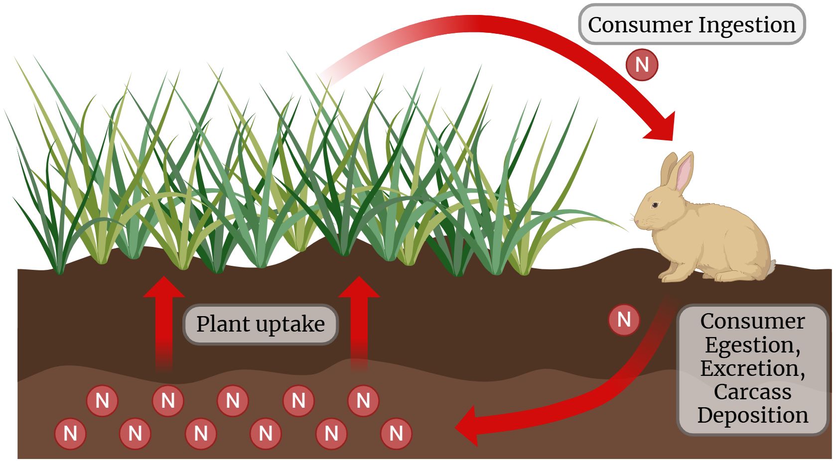
Figure 1. A nitrogen cycle involving plant and consumer interactions. Nitrogen is absorbed by plants from the soil, depicted as “Plant uptake.” A rabbit represents the consumer, which ingests plants; the process is labeled “Consumer Ingestion.” Arrows indicate nitrogen transfer, with the last going back to the environment through "Consumption, Egestion, Excretion, and Carcass Deposition." The interconnected arrows visually demonstrate the flow of nitrogen between soil, plants, and consumers. Source: Created in BioRender.com.

2 Key frameworks for understanding consumer-resource interactions

EST, DEB, and NG each offer distinct approaches to study consumer-resource interactions, yet differ in their motivations, perspectives, and key questions (Sperfeld et al., 2016, 2017; Kearney, 2021). In the following sections, we provide a brief summary of each framework to contextualize their usage in our model, especially for readers not familiar with all three.

2.1 Ecological stoichiometry theory

Ecological Stoichiometry Theory (EST) explores the connections between an organism’s elemental composition and their life history traits, interactions with other organisms, and impacts on ecosystem functioning (Urabe et al., 1997; Sterner and Elser, 2002; Anderson et al., 2005; Frost et al., 2005). Using elements as a currency for metabolic and ecological processes of interest is particularly useful when connecting mechanisms between organisms and/or ecological scales, such as the relationship between animal egestion and fertilized primary production. The ability to quantify how macroelements, such as N, flow throughout an ecosystem is an informative tool for describing consumer-driven nutrient cycling (Elser and Urabe, 1999, 1999; Sterner and Elser, 2002; Grover, 2004; Moody et al., 2018) and how feedbacks between consumers and their environment impact ecological and biogeochemical processes (Sitters et al., 2017; Filipiak and Filipiak, 2020; Elser et al., 2022; Koeve et al., 2024).

EST can also be used to predict the fitness consequences of elemental imbalance between an organism’s demands and what is available in their environment (i.e., stoichiometric mismatch) (Sterner and Elser, 2002). These consequences can occur in different ways. First, element deficiency (i.e., nutrient limitation) can suppress organism performance (e.g. growth rate, reproduction, etc.) relative to more elementally balanced diets (Sterner et al., 1992). Second, consumers face costs when dealing with an overabundance of some elements in digesting, egesting, excreting, and/or storing unneeded nutrients, which has been shown to induce trade-offs in organismal performance (Boersma and Elser, 2006). The effects of stoichiometric imbalances on individual performance, population dynamics, and whole ecosystems can often be isolated experimentally, but it can be difficult to interpret observational data where there are often multiple, interacting limiting nutrients. Here, EST can explicitly describe the dynamic shifts in elemental limitations through the concept of TERs. TERs are the resource elemental ratio at which an organism’s growth shifts from limitation by one element to another (Frost et al., 2006), allowing for a combination of elemental ratios to describe a “stoichiometric niche” of resources (González et al., 2017). If a consumer cannot meet these thresholds, it must adapt or face fitness consequences. The strategies for adapting to, and quantitative consequences of, elemental imbalances both lend powerful and complementary modeling concepts when used in conjunction with both NG and DEB frameworks (Sperfeld et al., 2017).

2.2 Dynamic energy budget theory

DEB theory is a mechanistic representation of an individual organism’s metabolism that directly links resource quantity and quality to its life-history traits by connecting resource composition to physiological processes (Kooijman, 2000). DEB models track how assimilated resources are stored in organisms (i.e., reserves) and then mobilized to pay metabolic costs for maintenance (i.e., overhead costs of maintaining current biomass), growth, and reproduction. Reserves provide a temporal buffer for consumers to sustain their metabolic function during resource fluctuations, effectively modeling individual-level nutrient hysteresis (Nisbet et al., 2000; Sousa et al., 2010). DEB theory also models concepts described by EST and NG, such as nutritional constraints on growth and reproduction (Muller et al., 2001, 2004; Kuijper et al., 2004) and consequences of resource switching (Kooijman, 2000). DEB models have already been integrated into ABMs to scale individual-level energetics to population dynamics (Martin et al., 2013), model zoonotic infection control scenarios (Malishev and Civitello, 2019), develop predictions for population management under climate change conditions (Yang et al., 2022), and better understand animal life history trajectories (Goedegebuure et al., 2018). For those unfamiliar with the intricacies of DEB, this section aims to present relevant assumptions, mechanisms, and modules available for DEB models that would be relevant to an ABM integrated with EST and NG concepts.

Two assumptions for DEB theory underlie its connection to biochemical composition of organisms: strong and weak homeostasis (Kooijman, 2000; Nisbet et al., 2000). Strong homeostasis dictates that metabolic pools within the organism do not change chemical composition (i.e., somatic structure, reserve pools, etc.). Weak homeostasis dictates that under constant resource density environments, the composition of the consumer as a whole remains static, implying that as resource quantity or quality varies, the reserve density (amount of reserve relative to the somatic structure, $m_{E} = \frac{M_{E}}{M_{V}}$ ) drives the overall chemical composition of the consumer. For example, an individual facing extended nutrient-poor conditions will have depleted reserves, and thus its reserve density will be much lower than an organism fed abundant, high-quality food (whose reserves will be at capacity). The difference in composition between reserves and structure determines the range of whole-body composition of an organism (i.e., heterotrophic consumers have a stricter compositional range than primary producers that can separately uptake inorganic nutrients) (Sousa et al., 2010). These theoretical tenets of DEB provide a complementary approach to EST’s description of the elemental homeostatic flexibility in producers and consumers.

DEB models can also use multiple reserves to represent different generalized pools of biochemical compounds (e.g., C-rich and N-rich reserves) (Kooijman, 2000). To convert fluxes from reserves of different stoichiometries into biomass products of different stoichiometries (i.e., somatic tissue), DEB theory uses “Synthesizing Units” (SUs) (Kooijman, 1998). SUs are mathematically analogous to enzyme kinetics and scaled functional responses: substrates arrive at the SU (i.e., reserve-C and reserve-N), and are “bound” to the SU, which converts them to a new product at a certain rate. In the process of this product formation, the SU will also produce “waste”, which is critical in using DEB to consider consumer impacts on nutrient cycles, as this is what comprises nutrient release to the environment. Importantly, this is yet another point of connection between DEB models and EST. SUs in DEB models have been used to explore the effects of N-limitation on copepod reproduction (Kuijper, 2004), phosphorus limitation on Daphnia growth (Muller et al., 2001), C, N, and phosphorus limitation in marine cyanobacteria (Grossowicz et al., 2017), and multi-trophic nutrient limitation in chemostats (Kuijper et al., 2004).

Historically, both EST and DEB practitioners have created models that highlight how each framework individually can create stoichiometric-explicit models that predict life-history trajectories of consumers under various resource qualities (Sterner, 1997; Frost and Elser, 2002; Andersen et al., 2004; Kuijper et al., 2004; Logan et al., 2004; Anderson et al., 2005; Peace et al., 2013). We want to stress, however, that the use of both frameworks simultaneously can develop more realistic model representations of elemental flows, which are critical when models cross different mechanistic, temporal, and spatial scales, akin to real ecological systems. For example, the use of reserves in DEB models provides an internally consistent mathematical tracking of true nutrient limitation—a consumer has a buffer to withstand eating low-quality food for periods of time before it begins to experience fitness consequences (Kooijman, 2000). Thus, DEB models are ideal for understanding the effects of temporally variable resource quantity and quality. Additionally, DEB models more adequately model the individual-level trade-off between how assimilated nutrients eventually are utilized for growth, reproduction, or excreta, which can map onto different life history strategies (such as emergency reproduction, Kooijman, 2000). Alternatively, DEB models in and of themselves cannot adequately model or interpret the feedback of elements between consumers and their environment. EST is more well-suited to explain the ecological significance of consumer-driven nutrient cycling and can capitalize on the consistent currency of elemental ratios to scale from individuals to populations and biogeochemical cycles (Schindler and Eby, 1997; Hessen et al., 2004; Van De Waal et al., 2010; Moody et al., 2018; Elser et al., 2022; Rizzuto et al., 2024). Finally, DEB models have already been explicitly connected to NG (Kearney et al., 2010; Kearney, 2012), and many DEB models are able to predict movement and organismal performance outcomes that are relevant to many NG concepts (Arnall et al., 2019).

2.3 Nutritional geometry

NG was developed as a framework for understanding how animals manage nutritional intake when faced with resources that are imbalanced in their macronutrients (e.g., carbohydrates, proteins) (Simpson et al., 1997). Additionally, NG can help understand driving forces of consumer-resource interactions, especially how these occur in spatially-explicit contexts. NG conceptualizes nutrient imbalances within a two-dimensional nutrient space. In this space, each animal has an intake target, reflecting its nutritional needs for processes such as maintenance and growth. As the animal consumes food, its position shifts within the nutrient space, depending on the nutrients it ingests (Anderson et al., 2020). In theory, an organism’s goal is to reach their intake target whilst limiting excess or deficient intake of any particular nutrient. Accordingly, NG can be used to make predictions regarding what behavioral strategies an organism may employ when faced with imbalanced diets. For example, populations of migratory Mormon crickets were found to cannibalize each other when they were deficient in protein and salt, but when these nutritional imbalances were relieved, cannibalism slowed (Simpson et al., 2006). Further, these specific imbalances were important drivers of the movement of these crickets through the landscape (Simpson et al., 2006), highlighting the important connections between individual nutrition and behavior.

While EST and NG are similar in that they both focus on nutrients, they use different measurements that have trade-offs in explaining ecological phenomena. NG directly examines macromolecules and connects biochemical nutrition to ecological dynamics (i.e., distinguishing between the carbon in lipids versus proteins), whereas EST uses elements as a proxy for nutrition and is thus able to directly compare data between different organisms and environments. The complementary concepts and distinctions between NG and EST have been further described elsewhere (Sperfeld et al., 2016, 2017; Anderson et al., 2020). Ultimately, NG’s focus on consumer feeding behaviors in response to resource variability is a critical aspect of modeling consumer-interactions in stoichiometrically imbalanced environments.

3 Consumer dynamic energy budget model details

3.1 Model overview

In our ABM, an individual consumer’s feeding decisions can be shaped by its elemental intake. Penalties for over- or under-consuming individual elements are implicitly prescribed by DEB and are dictated by an organism’s elemental reserves (i.e., C-rich and N-rich reserve). Thus, the ABM can be used to explore the fitness consequences of different feeding strategies—such as between diet-switching and compensatory feeding—as predicted by NG. For instance, under a selective feeding (diet-switching) strategy, a consumer may struggle to grow or reproduce if resource quality fluctuates among food choices (Anderson et al., 2020). Below, we outline the relevant concepts and important model decisions underlying the specification of the DEB model. All flux equations can be found in Table 1, and a more complete specification of the model can be found in the Supporting Material (Appendices A and B), along with code for solving the equations in R (Appendix C). Moles of C, C-mols, are used as the common internal currency for the organism to streamline mass balances, as all internal state variables contain some amount of C. Moles of N, N-mols, can be easily calculated from the stoichiometric parameters.

Table 1

Table 1. Flux equations.

Important DEB model decisions are listed briefly below.

1. There are two reserves: C-rich and N-rich. Both contain C, but only the N-rich reserve contains N.

2. Consumers ingest a single resource, but the stoichiometric concentration of C and N in the resource can vary. Thus, assimilation of C and N are separate processes, not dependent on the actual resource itself (all equally digestible). While this assumption is not necessarily realistic, it is always possible to create multiple resources with different assimilation dynamics in a different DEB model, and our goal was to use elemental stoichiometry as a common currency throughout the simulated ecosystem.

3. Four SUs are used to calculate somatic maintenance, maturity maintenance, somatic growth, and reproduction. Details are found in Appendix A in Supplementary Material.

4. An organism’s somatic maintenance costs are increased through movement, based on the distance walked and a penalty parameter that multiplicatively increases maintenance costs based on total movement (σ).

5. Somatic maintenance and maturity maintenance must be paid in order for the organism to stay alive. If what is mobilized from reserves is insufficient to pay for costs, then somatic structure will be broken down and used to meet costs for either somatic or maturity maintenance (“shrinking and regression”). Details in choice to break down structure for maturity maintenance can be found in Appendix A.

a. For simplicity, we assume that any unused mobilized structure is immediately returned to structure (van der Meer et al., 2022), and that there is 100% efficiency in using structure.

b. Note: one should consider setting a limit on how much somatic biomass can be broken down to meet maintenance costs. In our ABM, we determined that death would occur if an organism shrunk by 50% of its maximally achieved structural mass as a conservative estimate, based on previous DEB ABMs (Martin et al., 2013), but this is likely far too forgiving of a shrinkage penalty for mammals.

6. “Waste” refers to egestion, and “excretion” refers to any other output of elements from the consumer into the environment (e.g., carbon through respiration, N through urine, etc.).

3.2 Mass balance differential equations

The mass balance equations are represented as a system of ordinary differential equations (ODE) that model fluxes of nutrients ( $J_{x y}$ , mol C/day) (Equations 1–9). A diagram of these fluxes through the DEB state variables can be seen in Figure 2. Users altering equations (or implementing other DEB models of interest) should take care that these fluxes are “absolute” fluxes as referred to in DEB theory, simply indicating that they are not scaled by consumer biomass or volume.

Figure 2

The diagram illustrates a metabolic budget model divided into two main resource reserves: C-rich (labeled as (C)) and N-rich (labeled as (N)). Arrows indicate energy and resource flows, including egestion (W_C and W_N) and functional outputs (F). The processes include somatic maintenance (SU-S), growth (SU-G), developmental maintenance (SU-D), and reproduction (SU-R), with variables representing resource allocations and efficiencies. Dashed connections highlight optional pathways, emphasizing the intricate balance between resource utilization and maintenance functions within the system.

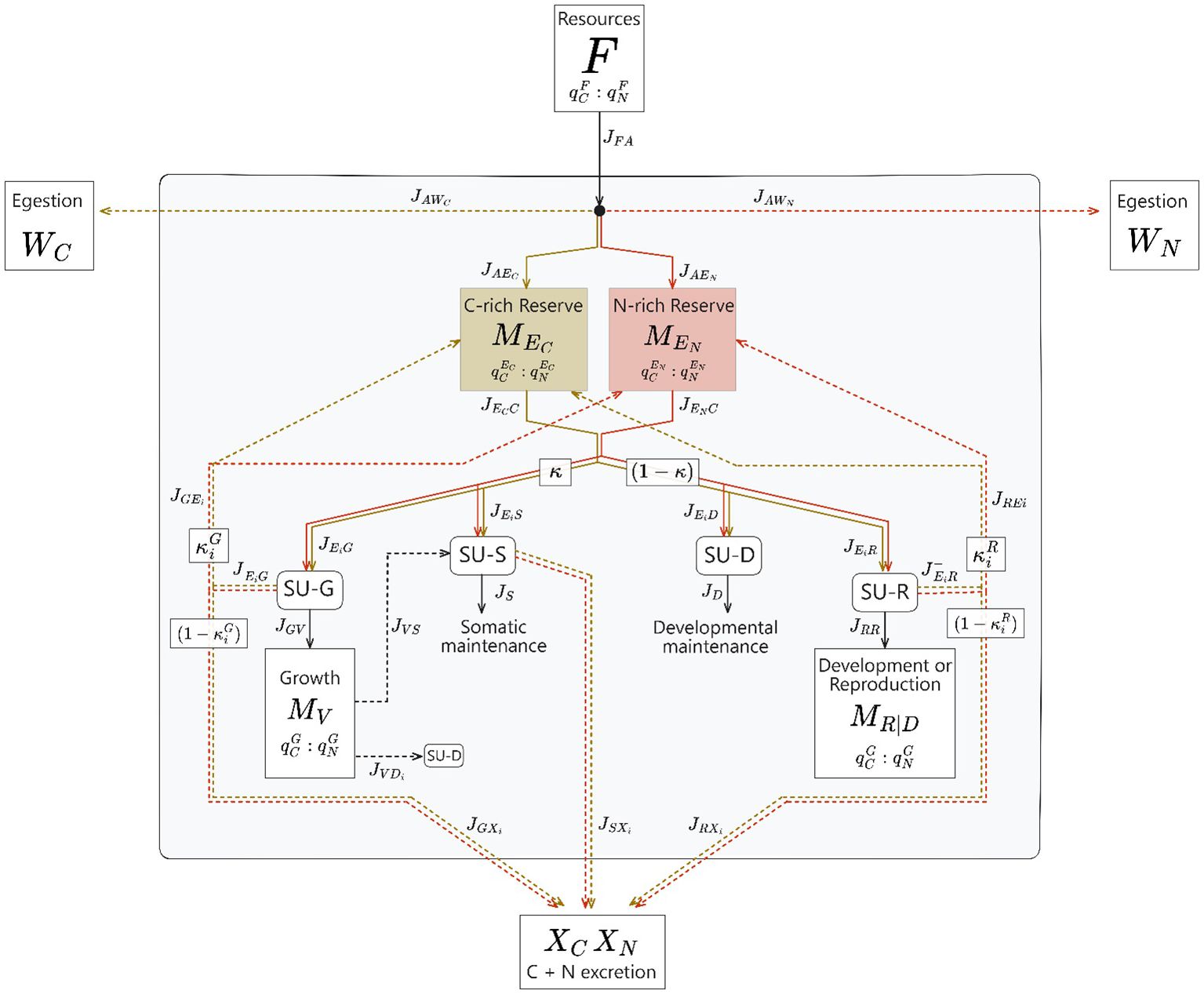
Figure 2. A diagrammatic overview of the Dynamic Energy Budget model presented in this paper. Resources with a quantified C:N stoichiometry are ingested by the heterotrophic consumer, and are then assimilated into a C-rich and N-rich reserve. Unassimilated resources are egested back into the environment. These reserves are mobilized to first pay somatic and developmental maintenance costs, then to grow and reproduce. Synthesizing Units (SUs) are described by DEB theory and combine fluxes of mobilized C- and N- reserves into a product flux with a fixed stoichiometry. Assimilated nutrients that did not yield maintenance costs, growth, or reproduction are excreted by the consumer.

\begin{array}{l} \frac{d M_{V}}{d t} = J_{G V} - J_{V S} - J_{V D} & (1) \end{array}

Somatic biomass increases due entirely to growth.

\begin{array}{l} \frac{d M_{E_{C}}}{d t} = J_{A E_{C}} + J_{G R E_{C}} - J_{E_{C} C} & (2) \end{array}

\begin{array}{l} \frac{d M_{E_{N}}}{d t} = J_{A E_{N}} + J_{G R E_{N}} - J_{E_{N} C} & (3) \end{array}

Reserve mass for both reserves (Equations 2, 3) increases through assimilation ( $J_{A E_{i}}$ ) and recycling of reserves mobilized but not utilized in the growth and reproduction processes ( $J_{G R E_{i}}$ ). Reserve mass is drained from the mobilization for growth and reproductive processes ( $J_{E_{i} C}$ ).

\begin{array}{l} \frac{d M_{H}}{d t} = J_{R R} i f M_{H} < M_{H}^{P}; 0 i f o t h e r w i s e & (4) \end{array}

\begin{array}{l} \frac{d M_{R}}{d t} = J_{R R} i f M_{H} \geq M_{H}^{P}; 0 i f o t h e r w i s e & (5) \end{array}

The reproductive maturity level ( $M_{H}$ ) increases from the development/reproduction flux $J_{R R}$ until it reaches the threshold to adulthood ( $M_{H}^{P}$ ). Once it has reached this threshold, $J_{R R}$ builds the reproductive buffer ( $M_{R})$ , which will produce offspring when it reaches the threshold for reproduction events ( $M_{R}^{0}$ ).

\begin{array}{l} \frac{d X_{C}}{d t} = J_{E_{C} S} + J_{E_{C} D} + J_{E_{N} S} + J_{E_{N} D} + J_{G R X E_{C}} + J_{G R X E_{N}} + J_{V S} + J_{V D} & (6) \end{array}

\begin{array}{l} \frac{d X_{N}}{d t} = (\frac{q_{N}^{V}}{q_{C}^{V}}) J_{E_{N} S} + J_{E_{N} D} + J_{G R X E_{N}} + (\frac{q_{N}^{V}}{q_{C}^{V}}) J_{V S} + J_{V D} & (7) \end{array}

Excretion of nutrients are released as a byproduct of the three metabolic processes that use multiple fluxes of different stoichiometries (somatic maintenance, growth, and development/reproduction). C-excretion fluxes are quantified in C-mols, and N-excretion fluxes are quantified in N-mols.

\begin{array}{l} \frac{d W_{C}}{d t} = J_{A W_{C}} & (8) \end{array}

\begin{array}{l} \frac{d W_{N}}{d t} = J_{A W_{N}} & (9) \end{array}

Egestion (“waste”) consists of ingested but unassimilated resources, and are also quantified in C-mols or N-mols, respectively.

All flux equations can be found in Table 1, a guide for terms and units can be found in Table 2, and all derivation steps/model choices can be found in detail within Appendix A in Supplementary Material.

Table 2

Table 2. Definition of terms.

4 Integrated agent-based model details

4.1 Model overview

NetLogo software (Wilensky, 1999) enables users to create spatially explicit ABMs and provides a user-friendly interactive coding environment to specify agent (i.e., consumer) behavior and metabolism, environmental conditions, with a well-established community of example models and code to users new to the program and ABMs as a whole. For longevity and new user ease, we have thus created our model in NetLogo, v6.4.

The ABM’s algorithms control the environment (patches) and consumers (agents). Algorithms are temporally divided into those that initialize the environment and consumers (“setup” procedures), and those that run each timestep (“tick”) of the model (“go” procedures), based on parameter specifications. For utility, many parameters that control (or impose) environmental and consumer mechanisms are displayed in the user interface. Below, we outline the procedures for the environment and consumers first in the initialization, then per timestep run in the model, and indicate how each of the three frameworks is either used to calculate values or contextualize assumptions for the procedures.

The NetLogo User Interface for this ABM contains three main sections: the parameter selection (Figure 3A), the environment (world) view (Figure 3B) and a set of plots and monitors that update each time step (Figure 3C).

Figure 3

Panel (A) displays user input controls, including options for patch and consumer configurations, with sliders and input fields for defining parameters such as initial conditions and resources. Panel (B) features an environmental view, illustrating a simplified landscape populated by blue and red points, representing different entities or resources within the modeled ecosystem. Panel (C) comprises data output graphs that track various metrics over time, such as total resources and consumer dynamics, showcasing trends and interactions within the simulation. The model facilitates exploration of ecological interactions through an interactive interface.

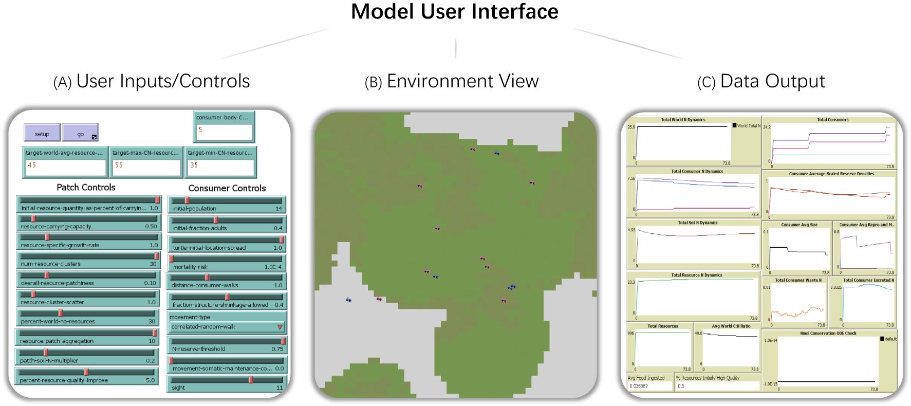
Figure 3. Preview of user interface for Agent-Based Model in NetLogo. Users directly enter the parameters for consumers and the environment, such as their stoichiometry, abundance, and spatial heterogeneity (A). Users can observe the simulated environment in real time as individual processes run and interact with agents and patches (B). Also included on the user interface are basic data plots of consumers and the environment which update each timestep (C).

4.2 Model initialization

The current model environment loads as a landscape with 25 × 25 patches, where the borders of the environment continuously wrap. The landscape is divided into patches that contain resources and those that do not. Resource patches can be further divided into a user-determined amount of high-quality clusters (e.g., heterogenous environment), or homogenous resource quality. The setup constrains the average C:N resource ratio over the whole world, within high-quality resource clusters, and lower-quality non-clustered resource patches, with user-determined target average, max, and min C:N ratios. We created spatial aggregation of resource patches and high-quality resource clusters by generating temporary agents at random patches, whose random walks determine which patches contain resources, and which resource patches are part of a high-quality cluster. For example, to assign high-quality resource clusters, the number of temporary agents generated is equal to the user-selected number of resource clusters. These agents take a total number of random walk steps that is equal to the user-selected area of each cluster. As these agents walk randomly, whichever patches they walk on get “converted” to the high-quality resource clusters. After performing these tasks, the agents are removed from the simulation. We also included a variable that incorporates random variation in all resource patches. Finally, we calculate the total C- and N-mol on each patch. For convenience, C-mol always is equivalent to the resource quantity parameter and N-mol is calculated from the C:N ratios of resources.

The total initial consumer population and proportion of adults vs juveniles are selected in the user interface. Once assigned a life stage, their initial DEB parameters are assigned, which the user specifies in the code. Then, initial state variable values are selected based on life stage, with user-specified variation or condition. Binary variables for consumers were also created to track important events, such as death (and cause of death), reproduction, and maturation.

4.3 Model run steps

A diagram summary of the ABM run procedures at each time step can be found in Figure 4. Each timestep corresponds to a day, based on the parameter units of DEB terms. Thus, we have discretized the ODE within the ABM to calculate per day and implement these calculations at every timestep.

Figure 4

The layout features a conceptual framework illustrating consumer processes, environmental impacts, and resource growth. In panel (C), the processes of ingestion and assimilation lead to metabolic activities influenced by various factors (F, N, R), resulting in maintenance (S) and reproduction (G). Panel (NG) denotes evaluation and movement processes. Below, environmental processes drive consumer impacts, updating resource quantity and soil nutrient pools while promoting biomass growth and nutrient uptake. The evolution of these processes is depicted across temporal panels (T0 to T3), indicating changes over time.

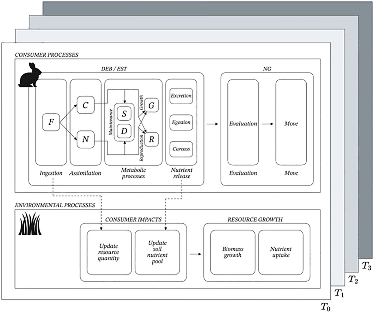
Figure 4. Overview of major procedures that occur each timestep in the Agent Based Model (ABM). The consumer completes its algorithm before the resource/patch submodel does to optimize the consumer nutrient feedback to resource growth. First, the consumer moves to a new patch, then ingests the resources on that patch. Then the DEB model calculates the change in consumer state variables for that timestep and determines mortality. If the consumer has accumulated enough energy, it will reproduce. Finally, the consumer releases to the patch its nutrients accumulated through excretion, egestion, and corpses. The ABM then updates the consumer and environmental variables, and executes a simple patch sub-model, where resources grow and their quality is calculated, depending on how much nutrients were deposited by consumers. The environment updates one last time before the next timestep begins.

All consumer procedures are the first to run at each timestep. Within the consumer procedures, first, all timestep-specific parameters are reset. Next, consumers move, based on sensing how full their N-rich reserve is (scaled reserve density). If the reserve is below a user-specified threshold (“mismatch_threshold”), then the consumer seeks out the best quality patch within a user-specified radius (“sight”) of patches and moves towards this target patch at a user-specified walk distance (“distance-consumer-walks”). Otherwise, the consumers will walk either in a correlated random walk (Renshaw and Henderson, 1981) or a Brownian walk (Kac, 1947) motion, based on user selection. Once at a patch, consumers’ ingestion potential is calculated based on a Holling Type II Functional Response. To avoid a patch having a negative number of resources due to multiple consumers’ ingestion, we implemented a rule that when multiple consumers are on a patch and there are not enough resources for all of them, consumers eat in turn, from largest to smallest, until no resources remain. After moving, an individual consumer’s DEB sub-model will compute the change in their state variables at that time step. To minimize NetLogo code clutter and utilize more advanced numerical solving algorithms, we used the SimpleR Extension for NetLogo (Hovet et al., 2022) to send parameters and state variables to an R script which calculates the change in state variables using the DEB sub-model, then sends the results back to NetLogo. Within our R script, we used the rootSolve package (Soetaert and Herman, 2009) and the `multiroot()` function, which performs Newton-Raphson methods to numerically solve variables (see Appendix A in Supplementary Material for more details on which variables need numerical solving methods). The roots solved in these equations are stored for each individual consumer at each time point, so that they can be used as the initial guesses in the next timestep, improving stability and solving efficiency. Following these root-solving calculations, consumer variables and relevant parameters are updated in NetLogo (i.e., the ODE is implemented as discrete calculations each timestep, essentially the Euler solving method). Based on the updated consumer states, if an individual exceeded (triggered) their thresholds for reproduction or death, those events occurred. Consumers can die due to a background mortality rate (set in user interface), both reserves reaching less than 1% capacity, or shrinking their biomass too significantly (threshold set in user interface, but we used 40% shrinkage per other DEB ABMs (Martin et al., 2013).

Next, environmental patches run their procedures. First, patches update how many resources were consumed and how much N was added to the soil pool by consumers. Then, patches will grow resources at a set rate each timestep, so long as they have not reached carrying capacity (rate and carrying capacity set in user interface). Resources uptake N from the soil at a certain rate (set in the user interface). To ensure that the C:N ratio of resources is maintained within the user-specified minimum and maximum, resource growth is constrained so that the resource C:N ratio cannot rise above the maximum and soil-N uptake is constrained so that the resource C:N ratio cannot dip below the minimum ratio. Then, the total C- and N- mols for resources and soil are updated again. Importantly, all procedures are written so that there is a world conservation of N, to better model where a known set of N is distributed throughout the system. This also provides a method for checking simulation experiments for numerical instability (N is not conserved from beginning to end).

Finally, all miscellaneous procedures run, such as assigning patch color based on the resource quality and updating plots, before the next timestep begins.

5 Case study: N limitation in snowshoe hares

5.1 Model overview and background

We modeled our case study around snowshoe hares (L. americanus) in boreal forests of North America (Krebs, 2010). We chose boreal forests since they are known to be N-poor environments (Sponseller et al., 2016; Högberg et al., 2017). Resource N limitation is known to influence snowshoe hare ecology, behavior, and physiology, and snowshoe hares are capable of modifying resource availability through herbivory (Rizzuto et al., 2021). Our model was designed to examine how hare population dynamics and ecosystem N cycling are influenced by variability in resource quality and hare feeding behaviors. Accordingly, we ran four distinct model scenarios, varying both environmental and consumer dynamics: (1) homogeneous vs. heterogeneous C:N molar ratios across the environment (see Sections 4.2 and 5.2) and (2) hare populations with either random feeding or N-selective feeding under N limitation (see Section 5.3).

5.2 Stoichiometric parameters

In all scenarios, the average resource C:N ratio initialized at 32, representing higher resource quality for relevant hare forage species (Rizzuto et al., 2019). Additionally, the maximum and minimum C:N resource ratios were arbitrarily selected to be 60 and 30, and the percent of world without any resources set to 30%. Under a heterogeneous resource conditions, the number of clusters was set to 20. Consumer C:N somatic biomass was set at 5, selected from a range of snowshoe hares at different ages (Rizzuto et al., 2019). For calculation convenience, the reproductive biomass C:N was set to be the same as the somatic biomass.

5.3 Behavioral parameters

We ran simulations across a factorial cross of two parameters: sigma (σ), which controls the multiplicative additional somatic maintenance costs of movement and also the N-rich reserve density threshold level at which consumers switch from a random correlated walk movement (random feeding) to seeking high quality food under N limitation (selective feeding, or, diet switching). For simplicity, we selected high values for both parameters: maintenance penalties for movement of 60% (sigma = 0.6) and thresholds for selective movement of 70% full reserves (scaled reserve density = 0.7). Other ABM parameters that were held constant are found in Appendix B in Supplementary Material.

5.4 DEB model parameter selection

Primary parameters for the DEB model were taken from the DEB Add-My-Pet Portal and used in a mass context with C-mols as common currency (Appendix B in Supplementary Material). While parameters for specifically L. americanus were not available in the database, we selected parameters from another cold-adapted species within the genus, the mountain hare (L. timidus). From these primary parameters, we calculated any other secondary DEB parameters using the energy-mass relationships described in Table 2 and “Notation and Symbols” section in Kooijman (2000).

To account for the fact that the primary parameters were derived for a single-reserve DEB model, we split the total maximum reserve density between the maximum reserve density of both our reserves: 40% of the total maximum reserve density was arbitrarily chosen for the maximum C-rich reserve, while the rest was used for the N-rich reserve. Additionally, we lowered certain parameters to generate qualitatively realistic dynamics around maturation and reproduction: maturation threshold for puberty, the size of an individual at birth, and thus needed to lower the cost of reproduction. We did this in part to ensure that we were more closely matching reproduction yearly dynamics with field observations of snowshoe hares (Snowshoe Hare Species Profile, Alaska Department of Fish and Game, n.d.). We calculated the cost of reproduction as the needed amount of C and N exactly to the size of a newborn plus its precocial maturity level (which we kept the same as the AMP Portal parameter) and reserves. For simplicity, consumers were all born with these same traits and scaled reserve density (0.9 for C-reserve and calculated ~0.86 for N-reserve). Births occurred when an adult consumer’s reproduction buffer reached the level of having a litter of 5. A full table of parameters used is in Appendix B in Supplementary Material, and the code to run the ABM is available in Appendix C in Supplementary Material.

5.5 Simulation experimental design

Within the model, N is cycled from resources to consumers through ingestion, then to a soil pool through consumer release (egestion and excretion), then back to the resources through uptake (Figure 1). We aimed to have a closed N system, though it is not necessarily realistic, so that we could ensure the model was numerically stable and track how N is shifted in different biomass throughout the simulation.

We used BehaviorSpace in NetLogo to perform these simulation experiments. Each simulation ran for 1000 time steps (i.e., 1000 days), with 10 replicates per parameter set. Replicates were needed to identify trends even among identical parameter sets, as consumers’ movement and the initialization of resource aggregation introduces stochasticity. Simulations ended early if no consumers were alive. The selected outputs were collected at each timestep from the simulations: total individuals as adults and juveniles, total resource quantity, total soil N, total resource N, and total consumer N, as well as the mean and variance of resource C:N, resource quantity, consumer size, consumer scaled reserve densities, consumer reproduction and maturity. We removed 3 replicates from the full set of simulations, due to the simulation becoming numerically unstable mid-run, potentially due to hardware constraints.

5.6 Simulation results and discussion

Across all model simulations, hare populations exhibited rapid population growth following model initialization, presumably driven by initially high resource availability (Figure 5). However, reproduction was slightly lower for hare populations that fed randomly in the environment with homogeneous resource quality (Figures 5A, B). Although adult hare numbers temporarily declined after the initial reproductive surge, populations rebounded as juvenile growth increased in all simulations (Figure 5C, D). While population growth (adult count) was similar between scenarios with homogenous and heterogenous resource quality, hare populations that fed selectively on N-rich resource patches during periods of N-limitation exhibited abundances ~2× higher than their randomly feeding counterparts (Figures 5C, D).

Figure 5

Panels (A) and (B) illustrate the effects of initial resource quality—homogeneous versus heterogeneous—on juvenile and adult counts over time, with both behaviors (selective in green, random in brown) shown. Panel (C) depicts changes in patch resource quantity, demonstrating a distinct trajectory based on resource quality. Panel (D) presents the resource C:N ratio, indicating variability in response to feeding behavior over the time series. Panel (E) shows resource nitrogen variance, suggesting stability in nitrogen levels irrespective of behavioral type across time steps.

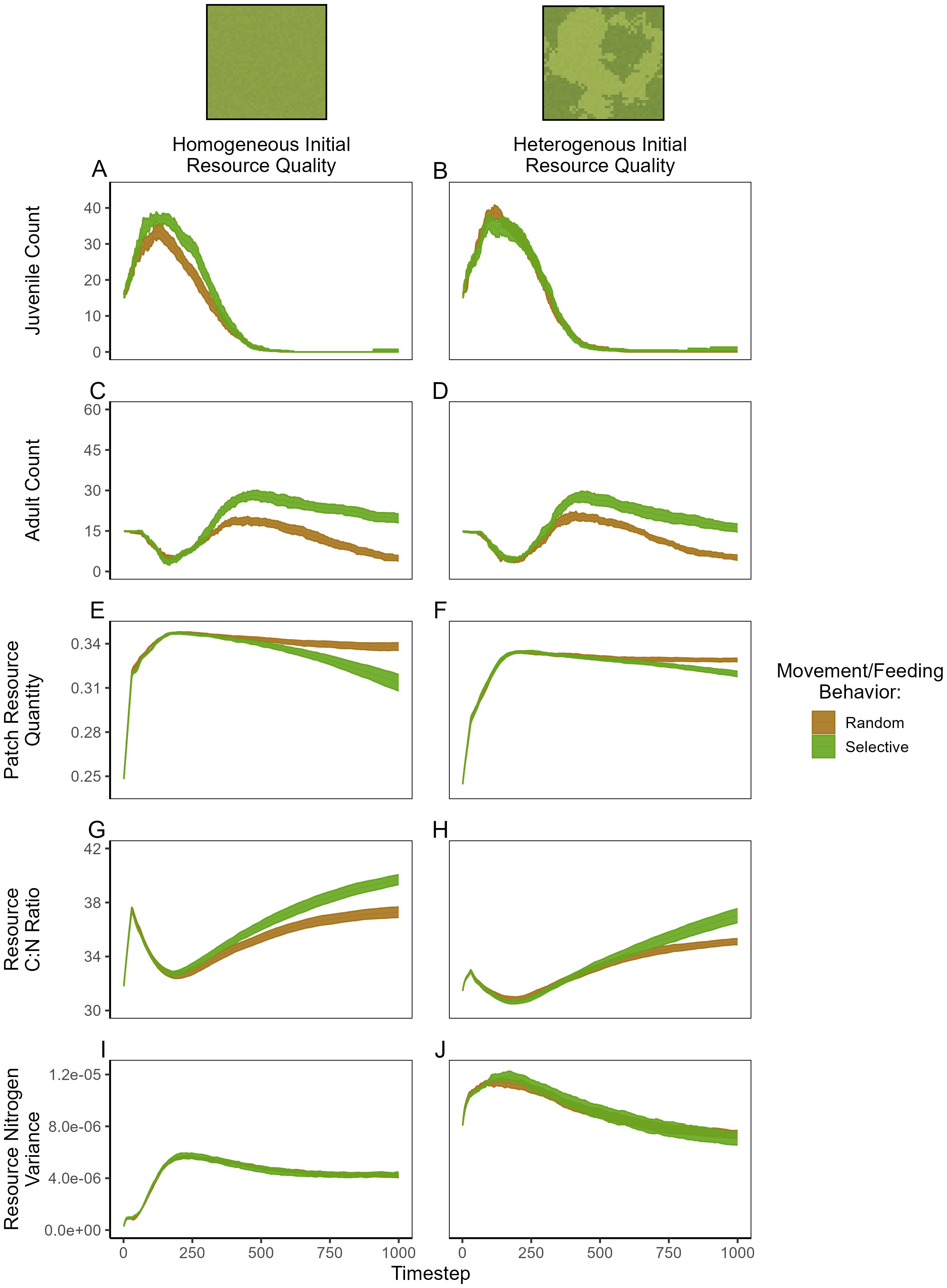
Figure 5. Summary of ABM simulation results exploring the effects of resource (nitrogen) heterogeneity and consumer feeding behavior (random vs selective) on population dynamics and nitrogen cycling. Each plotted line represents the mean value at each timestep from 10 replicate simulations and each ribbon represents the mean ± standard error. Variation between replicates arises from the stochasticity in consumer movement and specific initial resource aggregation.

While the heterogeneity of resource quality had only minor effects on hare population dynamics, it had important influence on N cycling and distribution by hare populations. Total resource consumption was higher for selectively feeding populations which exhibited greater abundances (Figures 5E, F) but was specifically highest for selectively feeding populations in the homogenous environment. Resource C:N ratios—reflecting resource quality—rapidly increased following initial plant growth but returned to baseline values following plant consumption during reproductive surges. However, resource C:N ratios eventually increased from starting values across simulations, reflecting an overall decline in resource quality (Figures 5G, H). Interestingly, this was most pronounced for selectively feeding populations, presumably due to the fact that these hares were able to seek out and consume N-rich resource patches.

Hare populations played an important role in generating and maintaining heterogeneity in resource quality—represented by the variance of N across the landscape (Figures 5I, J). Notably, hares dramatically amplified N heterogeneity in the initially homogeneous environment, and only marginally decreased N variance in the starting heterogenous environment. These effects occurred irrespective of feeding behaviors, suggesting a general importance of N transport by hare populations. As hares traversed the homogeneous environment, their waste and carcass deposition generated new high-N patches, amplifying the contrast between N-rich and N-poor areas. In contrast, within the heterogeneous environment, hares redistributed N from initial hotspots—first increasing heterogeneity by creating additional high-N patches but ultimately reducing heterogeneity below initial levels as their movement led to N deposition across the landscape (Figure 5I).

Ultimately, our model results suggest that the ability for hares to seek out N-rich resources when faced with N limitation significantly enhanced population fitness. While the initial heterogeneity of resource quality had only modest effects on hare population dynamics, its interaction with hare behavior strongly influenced patterns of N cycling. In general, hares reduced average resource quality through N consumption and increased spatial heterogeneity of resource quality. This case study thus also highlights the ability for researchers to study importance of consumers in distributing nutrients throughout the landscape.

6 Discussion and future directions

6.1 Model conclusions

We demonstrate how a multi-reserve DEB model within an ABM framework can be used to simultaneously explore the dynamic feedbacks among variable nutrient conditions, consumer traits, and population structure. These processes occur while maintaining physiological, spatial, and temporal specificity, akin to the complexity of real ecological systems. By parameterizing the DEB model using stoichiometric data and allowing for simulated consumers to behaviorally respond to their internal state, this approach provides a new integrative exploration of EST, NG, and DEB concepts. While we recognize that the general model outputs are highly dependent on the selection of parameter values (e.g., hare structural shrinkage allowed, environment spatial structure) and simplified ABM procedures (e.g., not allowing hares to remain in one patch over multiple timesteps), our primary aim here is to demonstrate how the model can help develop hypotheses about how stoichiometric imbalance influences populations and ecosystems. Furthermore, we believe it is most helpful to provide a basic set of procedures and broad parameter manipulation abilities so that other researchers can tune the model for different systems.

The results from our case study demonstrate the functionality of the model yet only touch the surface of the model’s utility to examine a broad range of questions across DEB, EST, and NG based on real world scenarios. Many novel anthropogenic changes to ecosystems, such as climate change, may affect consumer nutrition, energetics, and behaviors simultaneously (Van De Waal et al., 2010; Toseland et al., 2013; Diehl et al., 2022). Additionally, consumers have concomitant impacts on ecosystem functioning, indicating the importance of studying the impacts of anthropogenic change on zoogeochemistry (Abraham et al., 2023). Theoretical models offer valuable opportunities for understanding these challenges by generating testable hypotheses and making novel predictions. Such models are particularly useful when empirical data is difficult to obtain due to time, spatial scale, or logistical constraints. In cases where resources are limited, models can also help identify which variables are most critical to measure. Additionally, theoretical models allow for the exploration of complex feedback mechanisms that may be challenging to detect through experimental or observational approaches.

6.2 Key future model opportunities

Despite the intricacy and utility of our model, there remain many limitations that also highlight key areas of future integration. First, our model currently only reflects a two-trophic system, with one consumer population and a generalized primary producer community. Expanding the model to include predators and a more diverse consumer community would allow for a deeper understanding of how biodiversity and trophic complexity alter and are influenced by stoichiometric imbalances. For example, predator-prey interactions have been shown to substantially affect consumer population dynamics, movement and behavior, energetics, and nutrient cycling within ecosystems (Denno and Fagan, 2003; Schmidt et al., 2012; Kohl et al., 2015; Herzog et al., 2023). On the other hand, predator risk affects the physiology of prey which may result in higher metabolic rates as well as habitat shifts to fulfill their nutrient demands (Guariento et al., 2018). For example, grasshoppers under high predation risk increase requirements for energy from carbohydrates affecting the C of their food source as well as their C:N release by excretion (Schmitz et al., 2010). Additionally, while the model is already capable of measuring how consumers influence spatial availability of nutrients, it could be further developed to include specific spatial statistics (e.g., spatial autocorrelation, such as Morran’s I), an open-nutrient exchange landscape (e.g., nitrogen fixation, as opposed to the closed-nitrogen environment currently in the model), or environmental responses and feedbacks (e.g., primary productivity).

Second, our model currently only incorporates C:N ratios, reflecting prominent trade-offs between C-rich carbohydrates (energy) and N-rich proteins (nutrition). However, both the ABM and DEB sub-model are capable of modelling other elemental ratios, such as C:P, N:P, or micronutrients (i.e., Na, vitamins). For example, the reciprocal relationship between ribosome allocation and protein synthesis concurrently increases demands for P to maintain demands for growth (Hessen, 2008). Additionally, other micronutrients, such as Na, Ca, K, and Mg are gaining increasing attention for their contribution to ecophysiology and ecosystem functioning (Kaspari and Powers, 2016; Duvall et al., 2023). The immense amounts of elemental stoichiometry data including emerging data repositories, such as the STOICH database (STOICH Database Home, n.d), may be used to examine how a plethora of ecological outcomes differ under various simulated stoichiometric imbalance scenarios.

Third, our model can be used to examine theoretical outcomes under different behavioral scenarios and nutritional trade-offs, informed by NG approaches. Although our case study focused on consumer diet-switching responses, we developed the model so that a user can select between diet-switching and compensatory ingestion strategies. For example, shrimps can change their diet in low-P streams from C-rich detritus to P-rich insects and periphyton (Snyder et al., 2015), and many large vertebrates will constantly select for N, P, and Na-rich plants and other materials under nutrient stress (Duvall et al., 2023; Monk et al., 2024),. However, a consumer may also elevate their feeding rates and compensate for the insufficient food quality by higher food quantity (Jensen et al., 2012; Suzuki-Ohno et al., 2012; Flores et al., 2014; Anderson et al., 2020). In our ABM, users could compare the outcomes of compensatory feeding versus diet-switching behavior. For example, while diet switching may induce increased metabolic demands associated with food processing or increased movement, compensatory feeding may induce metabolic consequences associated with excess nutrient intake and processing. Adding these additional behavioral strategies can be used to examine which strategies are, in theory, more evolutionarily advantageous, and how these advantages may differ under various stoichiometric imbalance scenarios, especially those that play out in spatially heterogeneous landscapes (e.g., high vs low spatial heterogeneity of nutrients (Smith and Moore, 2003), high vs low N digestibility (Weiser et al., 1997).

6.3 Model caveats and lessons learned during design

Ecological systems are highly complex. Efforts to understand the intricacy of ecological interactions have ranged from generalized frameworks to complex ecological models. There are inherent trade-offs in each approach: general frameworks provide an intuitive way of describing nature, whereas complex models can attempt to provide realistic predictions that elucidate the importance of specific variables and mechanisms in ecological interactions (Sun et al., 2016). We recognize that our model lies on the latter end of this spectrum. Indeed, a general frustration with both ABMs and DEB models is their complexity and the number of parameters and individual-level processes included, creating compounding uncertainty in model outcomes (An et al., 2021). Regardless, the aim of this integrative model is to more accurately account for multiple processes when assessing the scaling effects of elemental imbalance—an outcome achievable only through increased model complexity. Since we aimed to make our model as user-friendly as possible to pull together researchers from different disciplines, we have tried to provide detailed descriptions of how we arrived at theoretical decisions, placed many important ABM parameters in the NetLogo User Interface, and designed the ABM and DEB sub-model to be mostly modular, such that researchers would be able to use the DEB model without needing to also use the ABM. Future research should compare our model outcomes with simpler models of DEB, EST, and NG to ascertain whether individual frameworks alone fail to produce the outcomes of the ABM as hypothesized.

The quality of model outcomes is also determined by the respective quality of empirical data needed for parameterization, particularly when trying to replicate real ecological systems. It is important that one must know enough about the biology of the organism to generate reasonable relationships between the parameters of two focal nutrients, or instead, have a tractable model system to collect enough of these parameters experimentally (e.g., Daphnia). DEB parameters can be estimated from empirical data (van der Meer, 2006), but are also available in a large database, Add-My-Pet portal (Marques et al., 2018). Users can install packages for downloading entries in the portal and work with their data through Matlab, R, and other programs. While many basic parameters can be extracted from the DEB Add-My-Pet portal for DEB models, it is still likely that one of the above strategies for parameter selection will need to be employed. Additionally, as more reserves, structures, and/or ontogenetic stages are added to the DEB model, the parameters increase, so parsimony in model design is needed for tractable calculations. Beyond consumer parameters, it can also be difficult to acquire sufficient environmental data for modeling abiotic and biotic nutrient cycling processes. For example, a challenge we faced in setting up our case study was determining the rates of nitrogen incorporation into soils and uptake by plants, for which data is lacking and can be highly context-dependent. Furthermore, users will need to appropriately tune the spatial and temporal scale of the model to match their respective system, as this will have important impacts on individual-level processes and their emergent effects as populations and communities. For example, in our case study, we use ‘days’ as a time unit based on the specific DEB parameters we chose, yet the ideal timescale will depend on focal systems, organisms, and questions.

6.4 Concluding remarks

In our model, consumers actively shape their environment by altering the distribution of elements and resources through space and time. A key advantage of the agent-based modeling (ABM) approach is its ability to simultaneously quantify the interactions between consumers and their environment. Variations in resource quantity and quality driven by organisms can significantly influence broader ecosystem functions, such as primary productivity, plant community composition, and biodiversity. These changes can create greater variability in the resources encountered at the individual level, generating long-term feedbacks that affect consumer populations.

Measuring the impacts of consumers on environmental heterogeneity is often challenging or even impossible in the real world at proper scale. For example, predicting consumer impacts on nutrient cycling must account for discernment between different nutrient release pathways (e.g., excrement, egestion, carcass deposition) including their variable rates and quantities. These measurements are largely unobtainable using field or observation methods, and thus, the ABM approach can provide a step towards a more realistic and holistic perspective on how consumers contribute to the heterogeneity of their environments, with bottom-up effects on ecosystem structure and function (e.g., primary productivity, habitat, biodiversity).

Ultimately, the integrative approach of our model presents new opportunities to explore concepts from EST, NG, and DEB, as well as other frameworks. The future directions we present here are only a selection of possibilities and opportunities. Continuation of model development by other users will ensure that modules are refined for specific landscapes (e.g., aquatic habitats), and how the wealth of stoichiometric, nutritional, and ecological data collected by our community can be combined to inform understanding and future study designs.

Data availability statement

The original contributions presented in the study are included in the article/Supplementary Material. Further inquiries can be directed to the corresponding author/s.

Author contributions

LB: Conceptualization, Investigation, Methodology, Project administration, Supervision, Validation, Writing – original draft, Writing – review & editing. ED: Conceptualization, Investigation, Methodology, Software, Visualization, Writing – original draft, Writing – review & editing. OA: Conceptualization, Investigation, Methodology, Visualization, Writing – original draft, Writing – review & editing. TNJ: Conceptualization, Investigation, Methodology, Visualization, Writing – original draft, Writing – review & editing. JJ: Conceptualization, Data curation, Methodology, Software, Validation, Visualization, Writing – original draft, Writing – review & editing. EW: Conceptualization, Investigation, Visualization, Writing – original draft, Writing – review & editing.

Funding

The author(s) declare financial support was received for the research and/or publication of this article. We thank the Alfred Wegener Institute (AWI), for hosting the guest research facilities of the Biologische Anstalt Helgoland during the WoodstoichV Workshop (grant number AWI_BAH_34). Participation of TNJ on this study and WoodStoich V workshop was supported by the Martina Roeselová Memorial Fellowship granted by the IOCB Tech Foundation. ESD would like to thank Cornell’s Department of Ecology and Evolutionary Biology’s Orenstein Fund for financing travel to the Woodstoich V workshop.

Acknowledgments

The authors would like to thank a number of individuals for their contribution to this work. This work was produced as part of the Woodstoich V workshop in ecological stoichiometry. We are grateful to the workshop organizers Cédric L. Meunier and Maarten Boersma, as well as the workshop mentors Robert Buchkowski, Cecilia Laspoumaderes, and Dieter Wolf-Gladrow. In particular, Dieter Wolf-Gladrow for helping with determining an appropriate root-finding numerical analysis protocol, and general enthusiasm for doing (what others would consider) tedious math problems. We also thank the reviewers immensely for their insightful feedback both scientifically and in the conceptual organization of the manuscript. This work would not be possible without LB’s training from David Civitello in DEB theory and co-development of multi-reserve DEB-EST models for LB’s dissertation. Additional gratitude to LB’s dissertation collaborator, Roger Nisbet, for his guidance and co-development of said models. We also thank Bas Kooijman for his time spent providing us insight over email correspondence during this project. Participation of TNJ on this study and WoodStoich V workshop was made possible thanks to David, Jonatán, Albert and Eduard and their endless patience with mommy’s projects. We also thank the Stack Overflow user Bryan Head for their strategy for creating landscape shapes in NetLogo.

Conflict of interest

The authors declare that the research was conducted in the absence of any commercial or financial relationships that could be construed as a potential conflict of interest.

Generative AI statement

The author(s) declare that no Generative AI was used in the creation of this manuscript.

Publisher’s note

All claims expressed in this article are solely those of the authors and do not necessarily represent those of their affiliated organizations, or those of the publisher, the editors and the reviewers. Any product that may be evaluated in this article, or claim that may be made by its manufacturer, is not guaranteed or endorsed by the publisher.

Supplementary material

The Supplementary Material for this article can be found online at: https://www.frontiersin.org/articles/10.3389/fevo.2025.1505145/full#supplementary-material

References

Abraham A. J., Duvall E., Ferraro K., Webster A. B., Doughty C. E., le Roux E., et al. (2023). Understanding anthropogenic impacts on zoogeochemistry is essential for ecological restoration. Restor. Ecol. 31, e13778. doi: 10.1111/rec.13778