Spatial distribution patterns and driving factors of ecosystem services and ecological vulnerability in ecologically fragile areas: a case study of the Zhang-Cheng area

Integrating ecosystem services (ES) and the ecological vulnerability index (EVI) to analyze the spatial distribution of ecological spaces provides valuable insights into promoting the sustainable development of ecologically fragile regions. To explore the spatial distribution patterns of ES and EVI in such areas, the Zhangjiakou-Chengde (ZC) area was selected as the study region. Four key ES—water yield (WY), soil conservation (SC), carbon sequestration (CS), and food supply (FS)—were assessed, and EVI was evaluated using the Sensitivity-Resilience-Pressure (SRP) model, with Z-score normalization revealing their spatial distribution patterns. The results showed that: (1) ES exhibited an increasing trend, while EVI decreased, with the most significant changes occurring between 2000 and 2010. Spatial patterns revealed that WY, SC, and CS increased from west to east, while FS and EVI decreased, with higher ecological vulnerability in the west; (2) Following Z-score normalization, ES and EVI were categorized into four quadrants: Quadrant I (High ES, High EVI) indicates areas with strong functions but high vulnerability due to human activities and climate change; Quadrant II (Low ES, High EVI) includes arid/semi-arid areas with high restoration potential; Quadrant III (Low ES, Low EVI) covers regions in need of ecological restoration; Quadrant IV (High ES, Low EVI) comprises areas with effective protection and low vulnerability; (3) Climate factors and land use changes significantly impacted the spatial distribution of ES and EVI. Interactions among multiple drivers, particularly in areas with intense human activities, amplified their effects. The findings offer important theoretical support for developing more precise ecological restoration and protection strategies and promoting sustainable development.

Highlights

● Integrated assessment of ecosystem services and ecological vulnerability.

● Z-score normalization method used for combining ecosystem services and ecological vulnerability index evaluations.

● GeoDetector applied to analyze drivers of ecosystem services and ecological vulnerability index spatial patterns.

1 Introduction

In the face of escalating global ecological challenges, the evaluation of ecosystem services (ES) and the ecological vulnerability index (EVI) has emerged as a pivotal focus in environmental science research. Ecosystem services—defined as the direct and indirect contributions of ecosystems to human well-being—are essential for sustaining life and promoting sustainable development (Costanza et al., 1997). Simultaneously, assessing ecological vulnerability is crucial for understanding ecosystems’ susceptibility to disturbances and their capacity for recovery, thereby informing effective conservation and management strategies (Adger, 2006). ES include functions such as water conservation, which ensures the availability of clean water for human and ecological needs (Costanza et al., 2014); soil retention, which prevents erosion and maintains soil fertility; and climate regulation, which helps stabilize local and global climate conditions. These functions are essential for maintaining ecosystem health and supporting the sustainable development of human society. However, with the intensification of human activities, pressures such as ecosystem degradation and climate change have made ecological vulnerability issues more prominent (Tang et al., 2021). Ecological vulnerability refers to the degree to which ecosystems are likely to be affected by natural or anthropogenic disturbances, encompassing both their sensitivity to such pressures and their capacity to resist or buffer against them, rather than simply their ability to recover from impacts (Weisshuhn et al., 2018). Therefore, both ES and EVI have become fundamental components of environmental research, as they jointly reflect the functional performance and the stability or fragility of ecosystems under changing environmental conditions (Xie et al., 2021). ES provides the healthy state and functions of the ecological environment, while EVI measures the ecosystem’s capacity to withstand and recover from stress. To gain a more comprehensive understanding of regional ecosystem status, combining ES and EVI for integrated assessment can better reveal the distribution patterns and dynamic changes of ecological spaces (Raheem et al., 2019).

Currently, significant progress has been made in the methods for assessing ES and EVI, and they have been widely applied in various ecological and environmental evaluations. ES assessment typically relies on quantitative models, remote sensing technology, and expert evaluations. Quantitative models, such as the InVEST (Integrated Valuation of Ecosystem Services and Trade-offs) model, have become important tools for assessing ecosystem services, particularly in functions related to water yield, carbon sequestration, and soil conservation (Jiang et al., 2016; Wang et al., 2022). The InVEST model can integrate factors such as land use, climate, and soil type to quantify the ecosystem services provided, offering scientific evidence for ecological protection and resource management (Ma et al., 2021). Additionally, remote sensing technology can acquire high-resolution surface imagery to monitor the spatial distribution and dynamic changes of ecosystems in real time, making it especially suitable for large-scale regional assessments of ES (Vargas et al., 2019). EVI evaluation typically relies on the Sensitivity–Resilience–Pressure (SRP) model, which comprehensively assesses ecological vulnerability by analyzing three key dimensions: Sensitivity, Resilience, and Pressure (Yang et al., 2021). Pressure refers to external stresses imposed on the ecosystem, such as climate change, land-use change, and pollutant emissions, with human activities being a major driving force (He et al., 2018). By incorporating climate and land-use scenario simulations, it is possible to predict how ecosystems may respond under varying pressure conditions (Shoyama and Yamagata, 2014). Sensitivity reflects the degree to which an ecosystem responds to external pressures—such as increased temperatures or altered precipitation patterns—and is influenced by topographic and climatic conditions (Gao et al., 2018). Resilience, on the other hand, represents the ecosystem’s capacity to absorb disturbances and maintain or quickly recover its structure and functions after stress, and is crucial for understanding long-term ecological stability (Mumby et al., 2014). Moreover, spatial statistical analysis methods, such as Geographically Weighted Regression (GWR) and GeoDetector, have also been widely applied in ES and EVI research to explore the spatial heterogeneity of ecological factors and socio-economic elements and their interactions (Gu et al., 2023; Wang et al., 2021).

However, despite the broad application of ES and EVI evaluation methods, existing research still tends to focus on single-dimensional analyses. Most studies assess ES or EVI separately, with fewer attempts to integrate both for comprehensive evaluation. Even when some studies attempt to combine the two, they typically use ES as an important indicator for EVI assessment, without fully considering the interrelationship between them. For example, some studies indirectly infer EVI by assessing changes in ES (Qiu et al., 2015). This approach overlooks the complex interactions between ES and EVI, and fails to fully reveal the ecological space distribution patterns jointly determined by the two. Ecosystems may exhibit both high levels of service and high ecological vulnerability, or conversely, low levels of service and low vulnerability. This phenomenon occurs when areas with significant ecosystem services, such as water yield or carbon sequestration, face heightened pressures from factors like climate change or human activities, increasing their vulnerability. Conversely, regions with lower ecosystem service potential may have lower vulnerability due to more stable or less exploited conditions (Malekmohammadi and Jahanishakib, 2017). Therefore, analyzing ES or EVI independently may lead to misjudgments regarding the ecological state. To address this gap, this study uses the Z-score normalization method to integrate ES and EVI, allowing for their combined evaluation. Z-score normalization effectively handles indicator data of different dimensions and units, and after standardizing them to a common scale (Deng et al., 2021). Z-score normalization helps reveal the combined spatial interaction patterns of ES and EVI.

In this context, the ZC area—a critical ecological barrier zone in northern China and a representative ecologically fragile area—was selected as the study region. This study aims to: (1) evaluate the spatiotemporal changes and interactions between key ES and EVI from 2000 to 2020; (2) integrate ES and EVI using Z-score normalization to classify the spatial distribution of ecological conditions into four distinct quadrants (High ES–High EVI, Low ES–High EVI, Low ES–Low EVI, and High ES–Low EVI); and (3) employ GeoDetector to identify and quantify the primary driving factors and their interactions influencing the spatial distribution of ES and EVI within each quadrant. These objectives are designed to provide a comprehensive understanding of how ES and EVI interact and evolve in ecologically fragile areas, thereby offering practical insights for regional ecological management and sustainable development planning.

2 Materials and methods

2.1 Study area

The ZC area is located in the northern part of Hebei Province, China (39°18′-42°37′N, 113°50′-119°15′E), serving as a key water source region and windward zone for both Beijing and Tianjin. The region covers an area of 7.63×10⁴ km² (Figure 1). It is characterized by diverse geomorphological types, including the northern Hebei mountain area, the northwest Hebei loess hilly region, and the Bashang Plateau, with terrain gradually descending from northwest to southeast. The climate is classified as temperate continental monsoon, with precipitation and temperature increasing from north to south. The mean annual precipitation ranges from 300 to 700 mm, and the mean annual temperature varies between -1°C and 9°C. According to the China Ecosystem Assessment and Ecological Security Database (http://www.ecosystem.csdb.cn/index.jsp), the ZC area is recognized as a plateau grassland and agricultural ecological zone, playing a crucial role in water conservation and soil erosion control in the Beijing-Tianjin-Hebei region. However, due to its location in the agro-pastoral transition zone, the region faces challenges such as water scarcity, overgrazing, grassland degradation, and soil erosion, rendering it a typical ecologically fragile area.

Figure 1

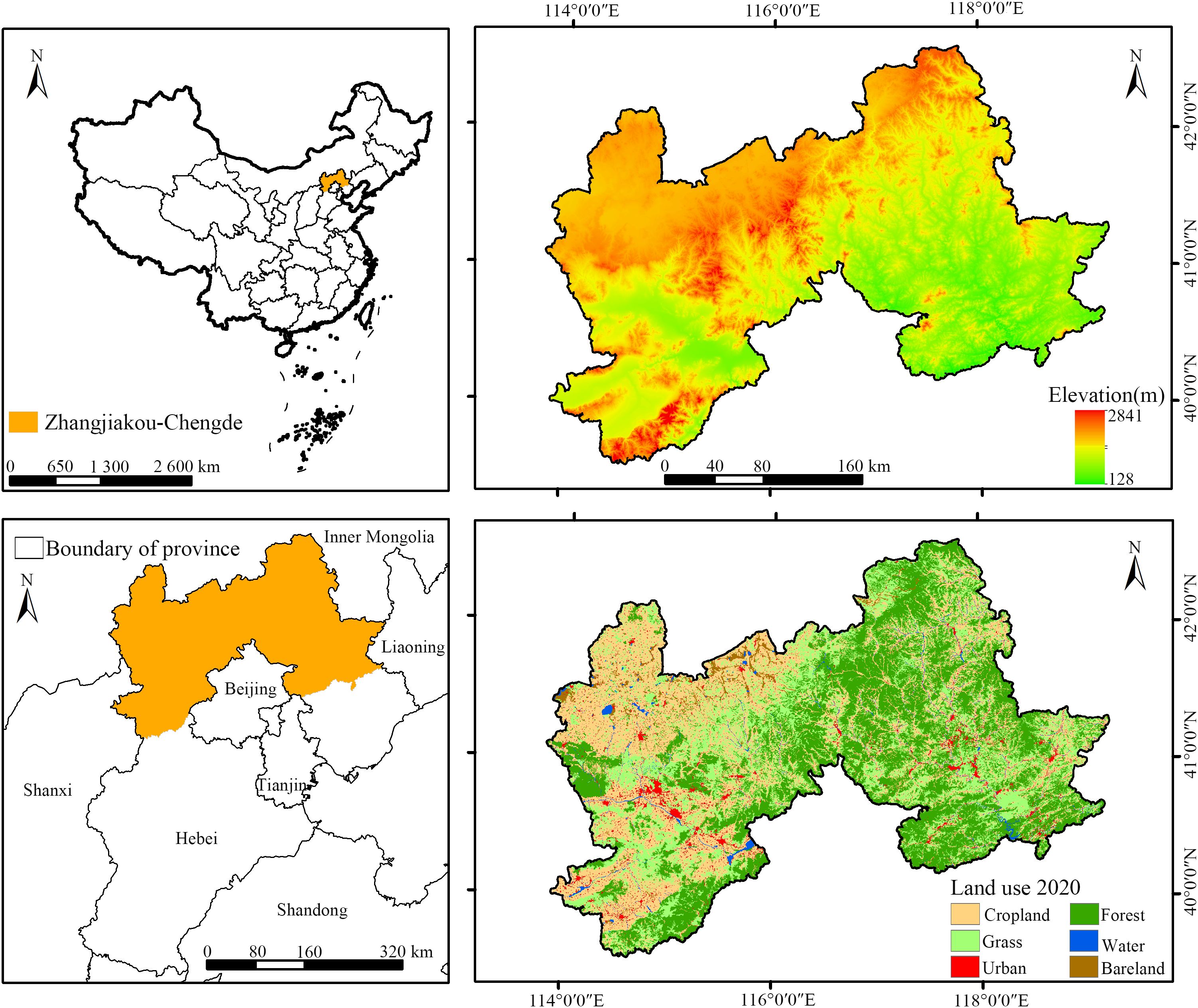
Figure 1. Location of the study site.

2.2 Data sources and preprocessing

The data for this study includes land use, meteorological, soil, vegetation index (NDVI), digital elevation model (DEM), and socio-economic statistics for the ZC area. Land use data is obtained from the Resource and Environment Science Data Center of the Chinese Academy of Sciences (https://www.resdc.cn/), which provides raster datasets for the years 2000, 2010, and 2020. The dataset classifies land use into six categories: cropland, forest, grassland, water bodies, built-up land, and unused land, with a spatial resolution of 30 m. Meteorological data is sourced from the China Meteorological Science Data Sharing Service Network (https://data.cma.cn/), including monthly precipitation and potential evapotranspiration data from 30 meteorological stations surrounding the study area, covering the period from 2000 to 2020. Soil data is derived from the World Soil Database (HWSD), specifically the “China Soil Dataset.” NDVI data is obtained from the National Ecological Science Data Center (http://www.nesdc.org.cn/), with a spatial resolution of 30 m. DEM data is acquired from the Geospatial Data Cloud (http://www.gscloud.cn/), with a resolution of 90 m. Socio-economic data primarily comes from the relevant years of the “China Urban Statistical Yearbook,” “China County Statistical Yearbook,” “Hebei Statistical Yearbook,” and statistical yearbooks from various prefecture-level cities.

Considering the environmental characteristics and data calculation requirements, the study area was divided into a 1 km × 1 km grid using the Fishnet tool in ArcGIS 10.8. The mean values for each grid cell were then extracted, resulting in a total of 7.62×10⁴ grid cells. These grid cells were used for the calculation and analysis of ecosystem services and ecological vulnerability.

2.3 Method

The workflow begins with data acquisition and processing, including land use, climate, soil, and socioeconomic data. This is followed by the assessment of four key ecosystem services: water yield, food supply, soil conservation, and carbon sequestration. Specifically, WY is calculated using the water yield module of the InVEST model based on the water balance principle; FS is estimated based on the significant linear relationship between crop yield and NDVI; SC is assessed using the Revised Universal Soil Loss Equation (RUSLE); and CS is evaluated through the InVEST carbon storage module. Afterward, Z-score normalization is applied to analyze the spatial distribution patterns of ES and EVI, categorizing them into four quadrants: Quadrant I (High ES, High EVI), Quadrant II (Low ES, High EVI), Quadrant III (Low ES, Low EVI), and Quadrant IV (High ES, Low EVI). Finally, GeoDetector is used to identify and assess the driving forces behind the spatial patterns of ES and EVI, including both single-factor and interaction effects (Figure 2).

Figure 2

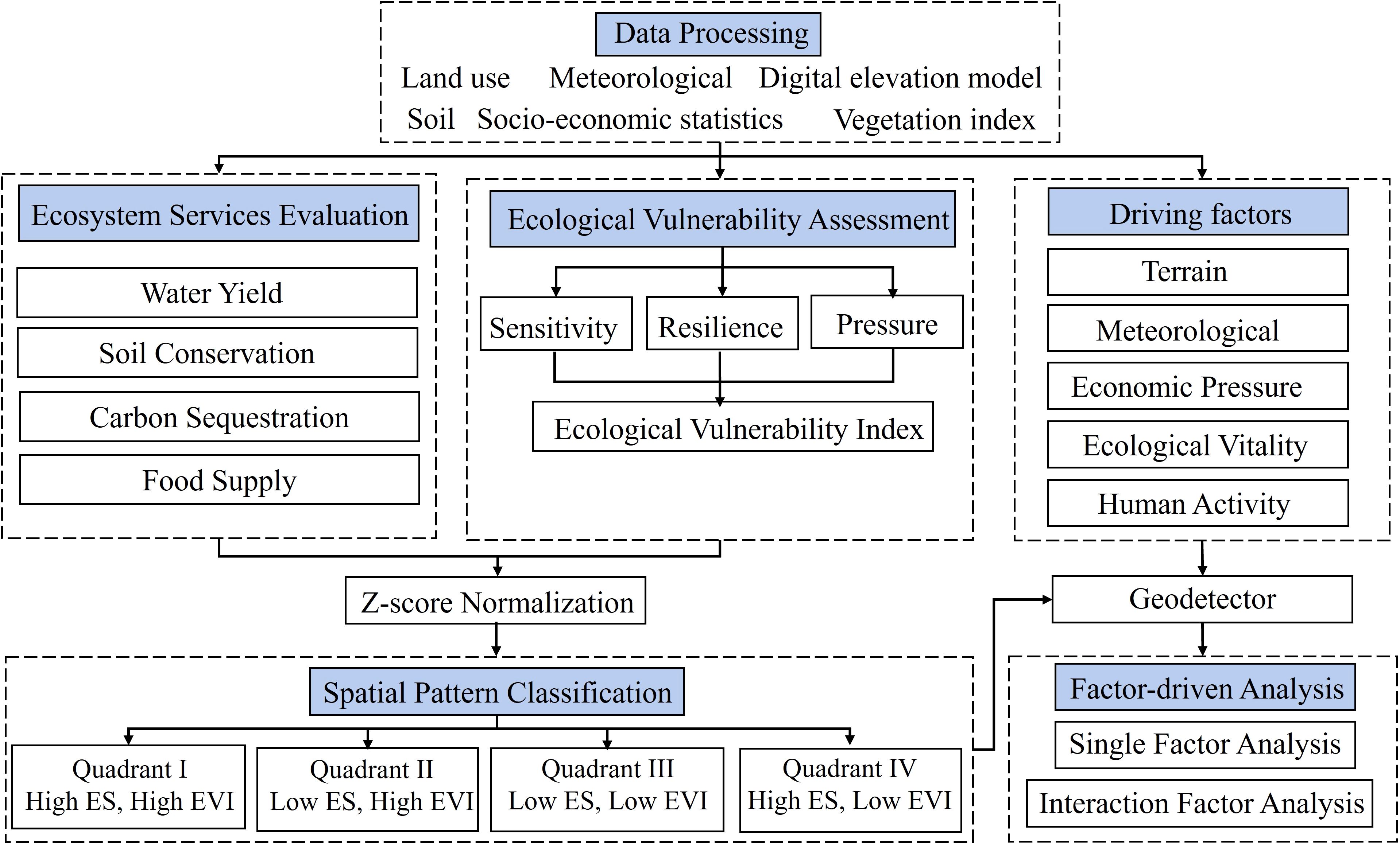
Figure 2. Methodology workflow.

2.3.1 Ecosystem services assessment

Based on the ecological functional zoning of the ZC area, this study primarily evaluates ecosystem services from the perspectives of provisioning and regulating services. As a major component of the water conservation zone within the Beijing-Tianjin-Hebei region, the ZC area plays a crucial role in freshwater retention and hydropower resource production (Zhou et al., 2023a). Additionally, as one of the main grain-producing regions in Hebei Province, it is of great significance for regional food security (Zeng et al., 2019). Therefore, water yield (WY) and food supply (FS) are selected as representatives of provisioning services. The ZC area is also a critical region for soil erosion control and an important carbon sink in the Beijing-Tianjin-Hebei region (Zhou et al., 2023a). Consequently, soil conservation (SC) and carbon sequestration (CS) are chosen as representatives of regulating services. The methods used for the ecosystem services evaluation are summarized in Table 1.

Table 1

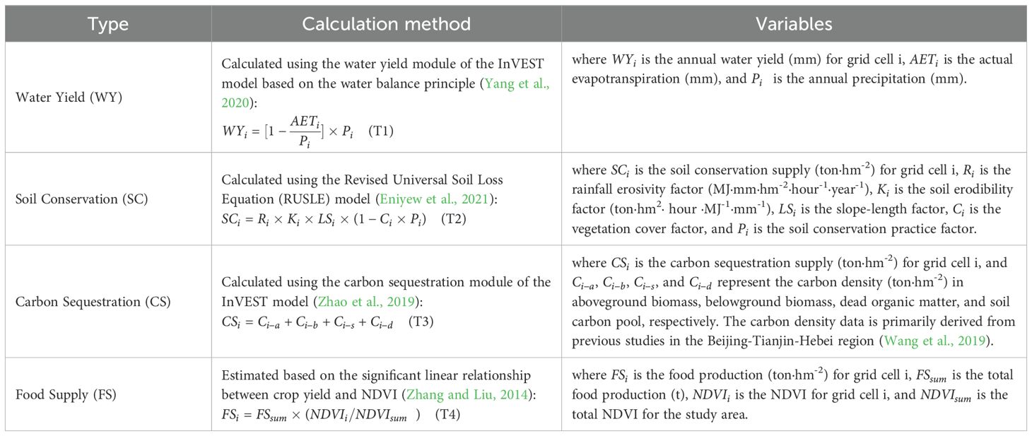
Table 1. Ecosystem services assessment methods.

2.3.2 Ecological vulnerability assessment

The ecological vulnerability assessment consists of four main steps: constructing the indicator system, normalizing the indicators, determining indicator weights, and calculating the EVI.

First, based on the Sensitivity–Resilience–Pressure (SRP) model for ecological vulnerability (Zou et al., 2021), and considering key ecological issues in the ZC area such as climate aridity and severe soil erosion, 13 indicators were selected (Table 2), with an emphasis on data timeliness and accessibility. The directionality of each indicator in the EVI system reflects its theoretical influence on ecosystem stability. A positive sign (“+”) indicates that higher values of the indicator are associated with increased ecological vulnerability, while a negative sign (“–”) implies a decrease in vulnerability. Specifically, terrain-related indicators such as ELV, SLP, and terrain TRI increase the difficulty of vegetation restoration and raise susceptibility to erosion and landslides, thereby increasing vulnerability. Similarly, climatic indicators including TMP, PET, and the SPEI indicate environmental stress due to heat and aridity. Human-related indicators, such as POP, LUDI, GDPP, and NTL, represent anthropogenic pressures that typically intensify ecological disturbance. In contrast, indicators with negative signs, including PRE, FVC, and RND, contribute to ecological resilience by improving water availability, stabilizing soil, and supporting vegetation growth. These directional assignments are based on prior ecological vulnerability frameworks and are tailored to the environmental characteristics of the ZC area (Weisshuhn et al., 2018). Sensitivity refers to the instability of an ecosystem when subjected to external disturbances, such as natural and human activities. Terrain and meteorological indicators are used to represent ecological change. Resilience refers to the ecosystem’s ability to recover from internal disturbances, with vegetation coverage and water system density chosen to reflect this. Pressure refers to the physiological effects resulting from external disturbances, often linked to human activities and economic factors. Indicators such as population density, land use intensity index (Zhang and Li, 2016), and gross domestic product are used to measure pressure.

Table 2

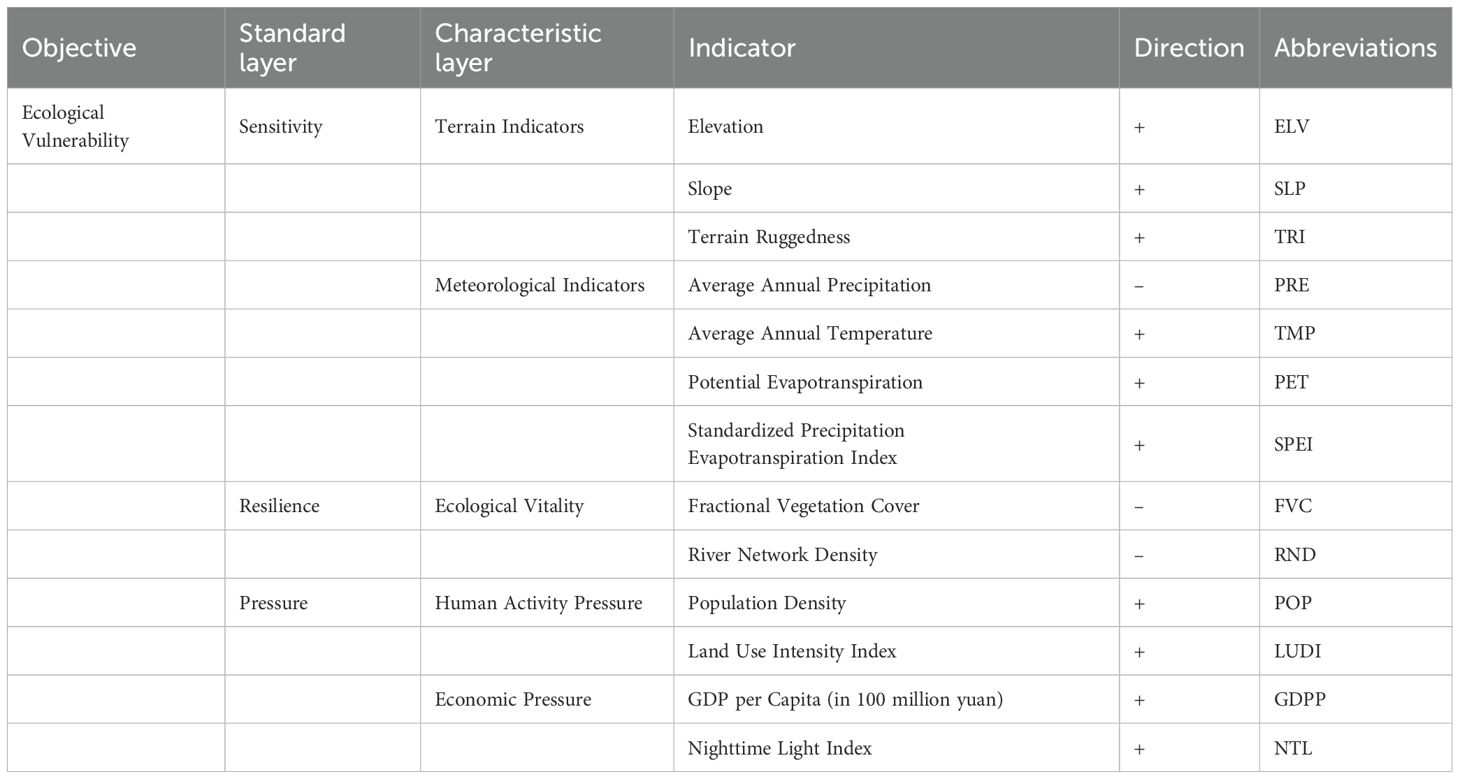
Table 2. Comprehensive ecological vulnerability evaluation indicator system for the ZC area.

Next, to eliminate differences in units and attributes across the indicators, the range normalization method was applied to standardize each indicator, transforming them into values between 0 and 1. The formulas used are as follows (Equations 1, 2).

$\begin{array}{ll}{X}_i^{+}=\frac{X_i-X_{i,min}}{X_{i,max}-X_{i,min}}& (1)\end{array}$

$\begin{array}{ll}{X}_i^{-}=\frac{X_{i,max}-X_i}{X_{i,max}-X_{i,min}}& (2)\end{array}$

Where $X_i^{+}$​ and $X_i^{-}$ are the normalized values for positive and negative indicators; $X_i$ is the raw value for indicator i; and $X_{i,max}$ and $X_{i,min}$ are the maximum and minimum values of indicator i.

Next, the Analytic Hierarchy Process (AHP) was employed to determine the weights of the indicators. First, indicators were categorized into three dimensions—sensitivity, resilience, and pressure—based on their ecological relevance and references from previous studies. A pairwise judgment matrix was constructed for each dimension through expert consultation and literature-based comparisons of relative importance. The consistency ratio (CR) was calculated to ensure the logical consistency of each matrix (CR< 0.1 was considered acceptable). Based on the normalized eigenvectors, the weights for sensitivity, resilience, and pressure were determined as 0.27, 0.42, and 0.31, respectively. All indicators were normalized to a scale of 0–1, and weighted aggregation was then applied to compute the composite EVI.

Finally, Principal Component Analysis (PCA) was applied to the normalized indicator matrix to reduce dimensionality and remove redundancy among the 13 indicators. Principal components with a cumulative contribution rate greater than 85% were retained. These components were then used to calculate the EVI by constructing a linear combination of the selected principal components, weighted by their corresponding eigenvalues. This approach ensures that the EVI reflects the most significant and uncorrelated sources of variation within the indicator set (Abson et al., 2012). Using a mathematical model, the weight of each indicator was determined, and the formula for calculating the EVI is as shown in Equation 3:

$\begin{array}{ll}EVI=r_1{y}_1+r_2{y}_2+r_3{y}_3+\cdots + r_n{y}_n& (3)\end{array}$

Where $y_i$ represents the normalized value of the i-th indicator factor, and $r_i$​ represents the weight of the i-th factor. After calculating the EVI, the result was normalized to ensure that the final value falls between 0 and 1. A higher value indicates greater ecological vulnerability.

In the SRP model, sensitivity was derived from terrain and climatic indicators (e.g., elevation, slope, precipitation), reflecting the ecosystem’s responsiveness to external stress. Resilience was measured by vegetation cover and water network density, representing the ecosystem’s capacity to recover. Pressure was estimated using socioeconomic and land use indicators (e.g., population density, GDP, land use intensity), which capture anthropogenic stress. To enable integrated spatial classification, ES and EVI—measured with different units and scales—were standardized using Z-score normalization. This transformation unified their values onto a common, dimensionless scale, making them directly comparable in quadrant-based spatial analysis.

2.3.3 Spatial distribution pattern analysis of ecosystem services and ecological vulnerability

Based on the two dimensions of ecosystem services and ecological vulnerability, the Z-score method was used to standardize the 7.62×10⁴ grid cells in the ZC area. The X-axis represents the standardized ecosystem service supply, while the Y-axis represents the standardized ecological vulnerability index. Based on this, the ZC area is divided into four ecological quadrants: Quadrant I (High-Supply, High-Vulnerability), Quadrant II (Low-Supply, High-Vulnerability), Quadrant III (Low-Supply, Low-Vulnerability), and Quadrant IV (High-Supply, Low-Vulnerability). The Z-score standardization formula is as shown in Equation 4:

$\begin{array}{ll}{Y}_i=\frac{X_i-\overline{X} }{S}& (4)\end{array}$

where $Y_i$ is the standardized ecosystem service supply or ecological vulnerability index for grid cell i; $X_i$ is the raw value for ecosystem service supply or ecological vulnerability index of grid cell i; $X_i$ is the mean of the ecosystem service supply or ecological vulnerability index; and S is the standard deviation.

This method effectively reveals the relationship between ES and EVI, simplifying their complex spatial distribution patterns into four intuitive categories. This helps in gaining a deeper understanding of their spatiotemporal changes and interactions.

2.3.4 Driver factor analysis

This study uses the Factor Detector and Interaction Detector from the GeoDetector method to quantitatively analyze the impact of various driving factors on the spatial distribution patterns of ES and EVI. First, ES or EVI was used as the dependent variable, and 13 evaluation indicators from the established index system were selected as independent variables. All variables were processed into 1 km × 1 km grid format to ensure spatial alignment. Then, each continuous independent variable was discretized into five levels using the natural breaks classification method, transforming numerical data into categorical variables suitable for GeoDetector analysis. These classified variables were then input into the GeoDetector model to evaluate their explanatory power for ES and EVI patterns. The Factor Detector was used to assess the individual explanatory power of each driving factor on the spatial differentiation of ES and EVI. The output is represented by a q-statistic, which ranges from 0 to 1. A higher q-value indicates that the factor has stronger explanatory power in accounting for spatial variation in the dependent variable. To identify the most critical drivers of ecological vulnerability, we compared the q-values across all 13 candidate variables. Those with the highest q-values in each quadrant were considered to have the greatest influence on EVI under specific spatial ecological conditions.

In addition, the Interaction Detector was used to evaluate whether the combined effect of two variables enhances or weakens explanatory power. Interaction types were classified into five categories: independent, univariate weakening, univariate enhancement, bi-factor enhancement, and nonlinear enhancement (Zhang et al., 2022), as shown in Table 3. This allowed us to determine not only which individual factors were influential, but also how combinations of climatic, topographic, and anthropogenic variables interact to shape ecological vulnerability.

Table 3

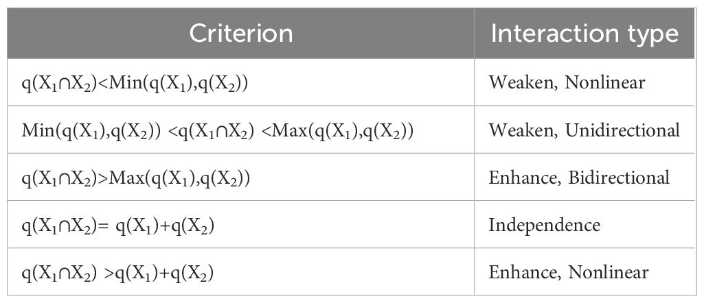
Table 3. Classification of interaction detector interaction types.

3 Results

3.1 Spatiotemporal changes in ES and EVI

Figure 3 shows the spatial patterns of key ES in the ZC area. WY, SC, and CS decreased from east to west, whereas FS showed the opposite trend, decreasing from west to east. From 2000 to 2020, WY and SC mainly increased in the eastern part of the ZC area, with the largest increases of 21% and 15%, respectively, while decreases were observed in the western part of the region, with the largest reductions of -40% and -23% (Figures 3d, h). During this period, CS and FS mainly increased in the western part of the ZC area, with the largest increases of 45% and 22%, respectively, while the areas of decrease were smaller (Figures 3l, p).

Figure 3

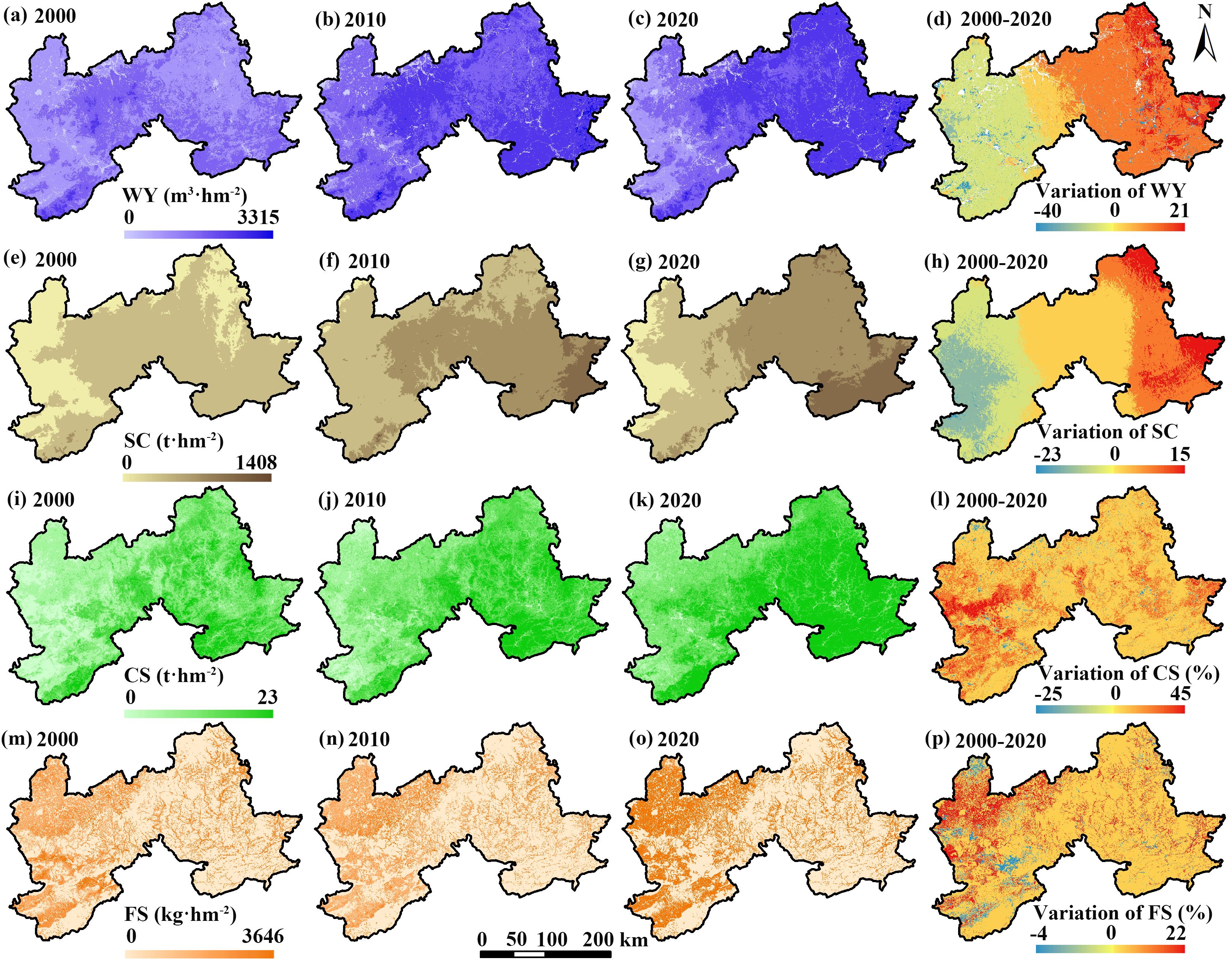
Figure 3. Spatial changes of various ES in the ZC area from 2000 to 2020. (a) WY in 2000, (b) WY in 2010, (c) WY in 2020, (d) Variation of WY from 2000 to 2020, (e) SC in 2000, (f) SC in 2010, (g) SC in 2020, (h) Variation of SC from 2000 to 2020, (i) CS in 2000, (j) CS in 2010, (k) CS in 2020, (l) Variation of CS from 2000 to 2020, (m) FS in 2000, (n) FS in 2010, (o) FS in 2020, (p) Variation of FS from 2000 to 2020.

Figure 4 shows the spatial variation of the EVI in the ZC area, which exhibited a high-to-low spatial distribution from west to east. From 2000 to 2020, EVI decreased in the eastern part of the region, with the maximum decrease of -30%, while it increased in the western part, with the largest increase of 45% (Figure 4d).

Figure 4

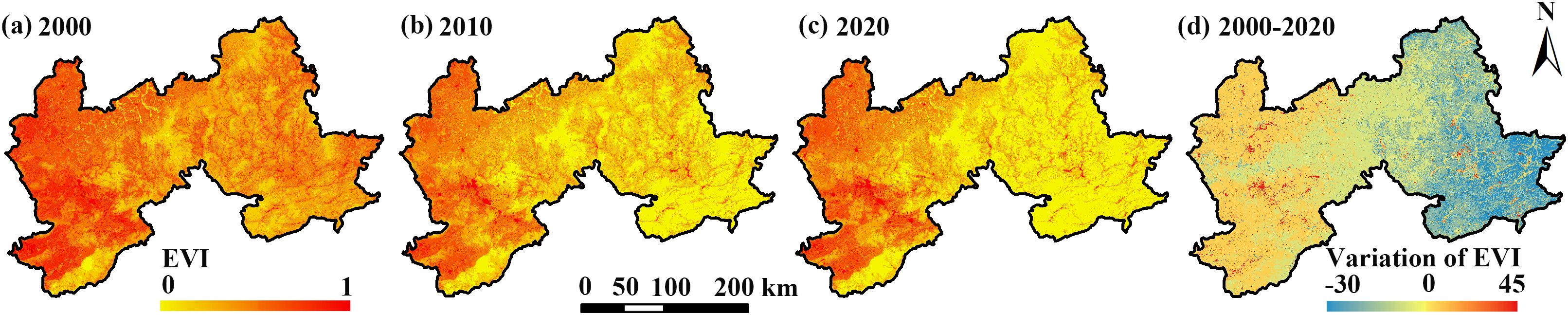
Figure 4. Spatial changes of EVI in the ZC area from 2000 to 2020. (a) EVI in 2000, (b) EVI in 2010, (c) EVI in 2020, (d) Variation of EVI from 2000 to 2020.

The values of ES and EVI over time (Figure 5) show that the mean values of key ES increased by 46.3%, while EVI decreased by 12.5%. The rates of change in ES and EVI indicate that WY, SC, and FS had the largest average increases from 2000 to 2010, while their average increases weakened in the 2010-2020 period. The increase in CS was nearly the same during both 2000-2010 and 2010-2020. The decline in EVI mainly occurred during 2000-2010, while there was almost no change in EVI during 2010-2020. Although the average EVI in the ZC area decreased from 2000 to 2020, the western part still maintained relatively high ecological vulnerability.

Figure 5

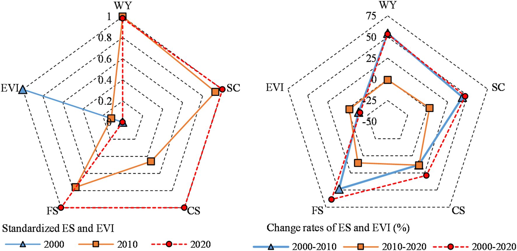
Figure 5. Temporal changes of various ES and EVI in ZC area from 2000 to 2020. (a) Temporal changes of standardized ES and EVI, (b) Change rates of ES and EVI.

3.2 Correlation analysis between ES and EVI

Figure 6 presents Pearson correlation results between ES types and EVI. All ES pairs were significantly correlated (p< 0.01). WY-SC, WY-CS, and SC-CS showed positive correlations, while WY-FS, SC-FS, and CS-FS showed negative correlations. Over time, the positive correlations between WY-SC, WY-CS, and SC-CS strengthened, while the negative correlations between WY-FS, SC-FS, and CS-FS became more pronounced. ES and EVI also showed significant correlations (p< 0.01).

Figure 6

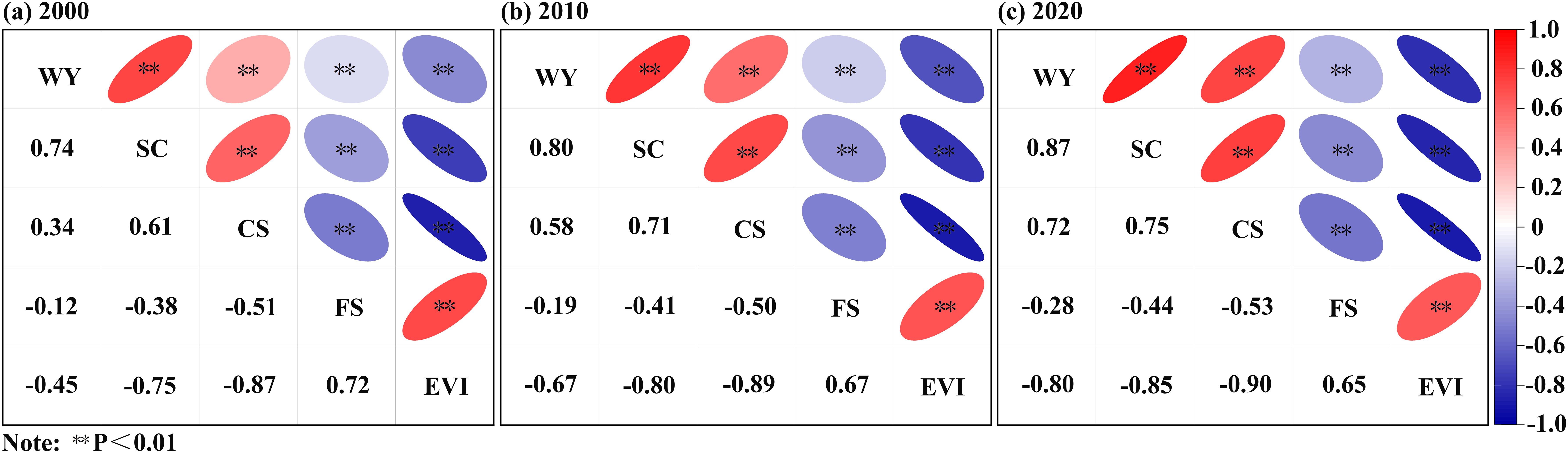
Figure 6. Correlation between various ES and EVI in the ZC area from 2000 to 2020.

A positive correlation was observed between FS and EVI, while negative correlations were found between WY-EVI, SC-EVI, and CS-EVI. Over time, the positive correlation between FS and EVI weakened, while the negative correlations between WY-EVI, SC-EVI, and CS-EVI strengthened. Among the ES types, FS was negatively correlated with other services, indicating trade-offs, and this trade-off relationship weakened over time. The relationships between WY, SC, and CS were positively correlated, indicating synergies, and this synergistic effect strengthened over time. The negative effects of WY, SC, and CS on EVI increased over time, while positive impact of FS on EVI decreased.

3.3 Spatial distribution patterns of ES and EVI

Figure 7 shows the quadrant-based spatial distribution of ES and EVI, derived from Z-score normalization. The spatial patterns of WY-EVI, SC-EVI, and CS-EVI were consistent. In 2000, more than 65% of the region was categorized as Quadrant II (Low ES, High EVI), suggesting low service supply coupled with high vulnerability. By 2010, a considerable portion of the region shifted to Quadrant IV (High ES, Low EVI), particularly in the central and eastern parts, indicating both ecological improvement and vulnerability reduction. This pattern remained largely stable through 2020, with Quadrant IV slightly expanding.

Figure 7

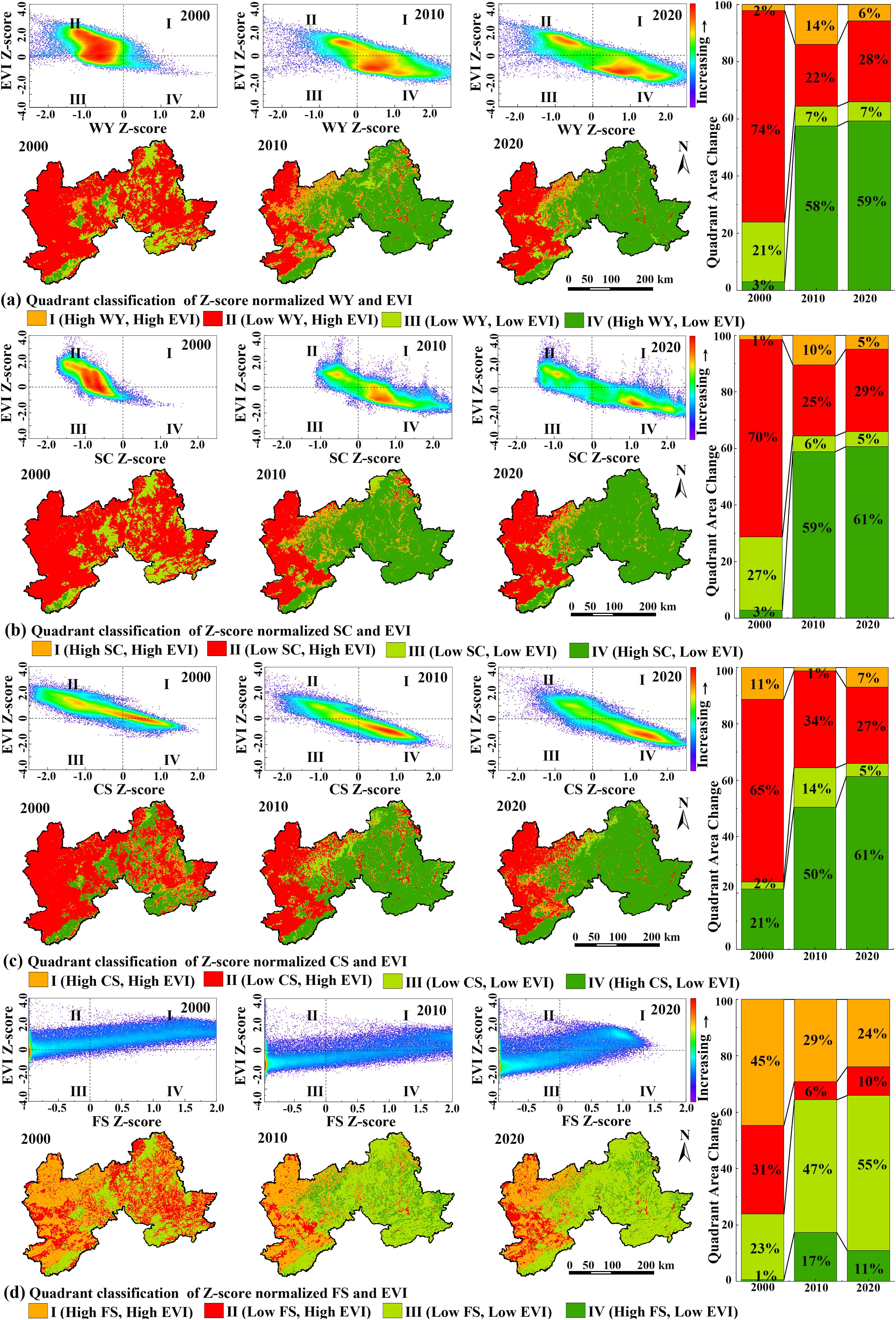
Figure 7. Spatial distribution patterns of various ES and EVI in the ZC area from 2000 to 2020 based on Z-score normalization and changes in the area of each quadrant. (a) WY and EVI, (b) SC and EVI, (c) CS and EVI, (d) FS and EVI.

The spatial distribution pattern of FS-EVI was different. In 2000, FS-EVI was mainly distributed in Quadrants I (High FS, High EVI) and II (Low FS, High EVI), covering 76% of the area. This indicated that the region had strong food production capacity, but also high ecological vulnerability. In 2010, large areas in the eastern and central parts of the ZC area shifted from Quadrants I and II to Quadrants III (Low FS, Low EVI) and IV (High FS, Low EVI), indicating that although FS had improved, EVI had decreased. By 2020, the area in Quadrant III continued to increase, while the area in Quadrant IV declined compared to 2010.

Figure 8 presents the integrated ES-EVI spatial distribution based on average Z-scores. In 2000, over 70% of the area (54 817 km^²) fell into Quadrant II. By 2010, large regions shifted from Quadrants II and III into Quadrant IV, especially in the eastern and central parts. In 2020, both Quadrants I and IV expanded, with the expansion of Quadrant I primarily resulting from increased ES supply without a proportional decrease in EVI (Figure 9).

Figure 8

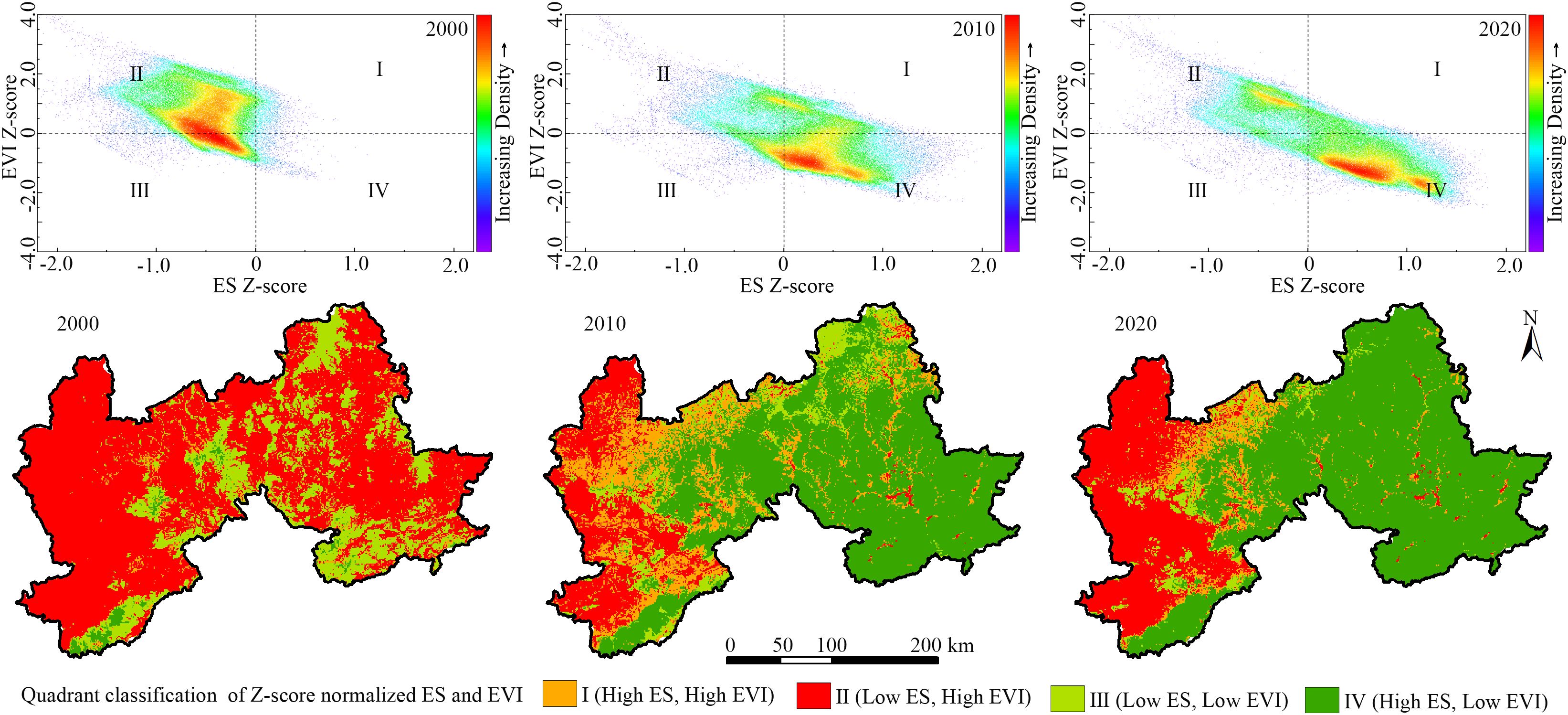
Figure 8. Spatial distribution patterns of integrated ES and EVI in the ZC area from 2000 to 2020 based on Z-score normalization.

Figure 9

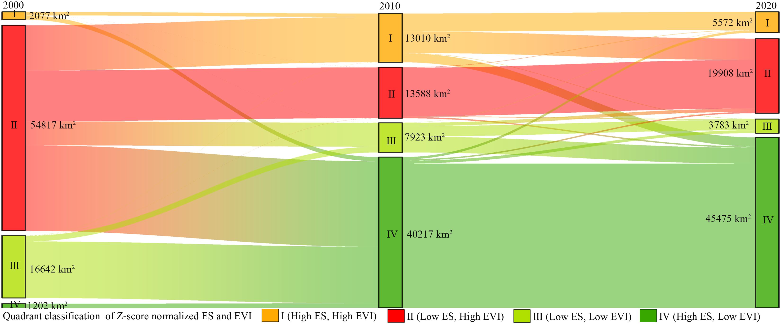
Figure 9. Sankey diagram of area transfer among quadrants in the ZC area from 2000 to 2020.

3.4 Driving forces of the spatial distribution patterns of ES and EVI

Figure 10 presents the results of GeoDetector’s single-factor analysis of 13 potential driving factors affecting ES and EVI in different quadrants.

Figure 10

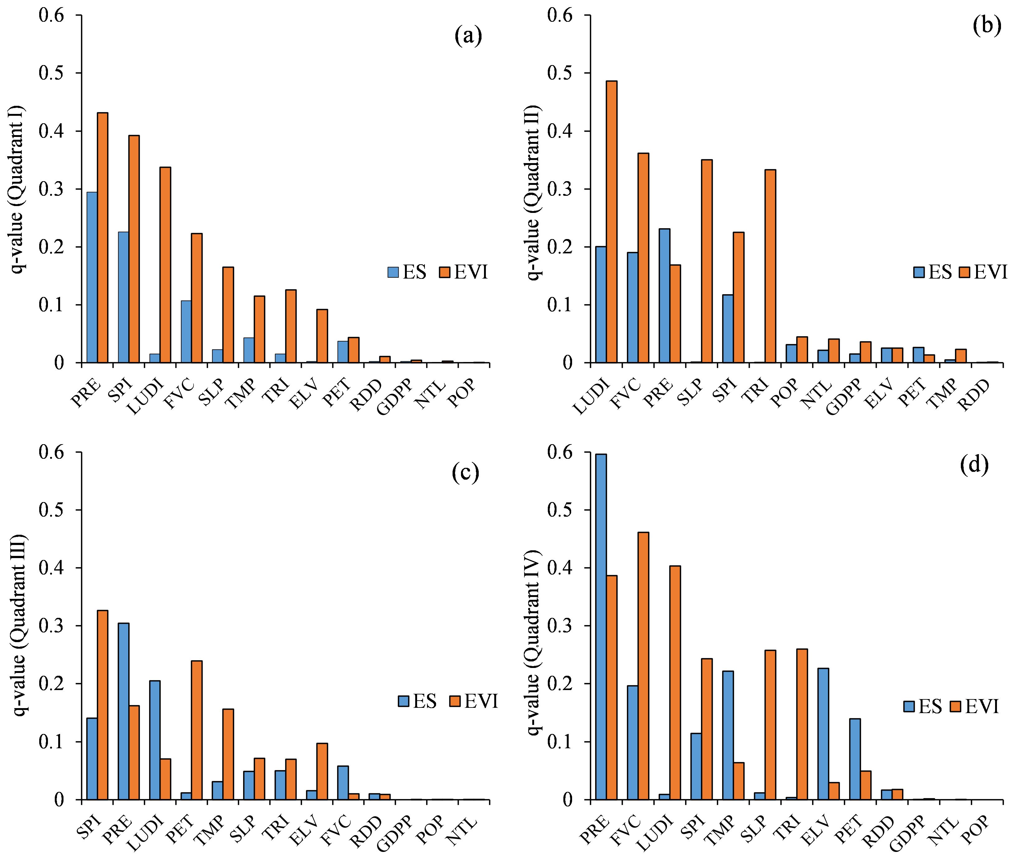
Figure 10. Q-value of driving factors on ES and EVI in each quadrant: (a) I; (b) II; (c) III; (d) IV.

In Quadrant I, the main influencing factors for ES were PRE (q = 0.29), SPI (q = 0.23), and FVC (q = 0.11), while the top drivers for EVI were PRE (q = 0.43), SPI (q = 0.39), and LUDI (q = 0.34). In Quadrant II, PRE, LUDI, and FVC had the highest explanatory power for ES, while LUDI (q = 0.49), FVC (q = 0.36), and SLP (q = 0.35) were most influential for EVI. In Quadrant III, PRE, LUDI, and SPI were the top drivers of ES, while SPI, PET, and PRE explained most of the variation in EVI. In Quadrant IV, PRE (q = 0.60), ELV, and TMP were dominant for ES, while FVC, LUDI, and PRE had the strongest influence on EVI.

Figure 11 illustrates the interaction effects among drivers. The combined explanatory power of any two variables was greater than that of individual ones, indicating bi-factor or nonlinear enhancement. For example, in Quadrant I, key interactions included PRE∩LUDI (q = 0.40), PRE∩SLP, and PRE∩FVC. For EVI in the same quadrant, the most significant interactions were LUDI∩SPI and LUDI∩PRE (q = 0.65 each). Similar patterns were observed across other quadrants, underscoring the synergistic influence of climate and land use on ES and EVI patterns.

Figure 11

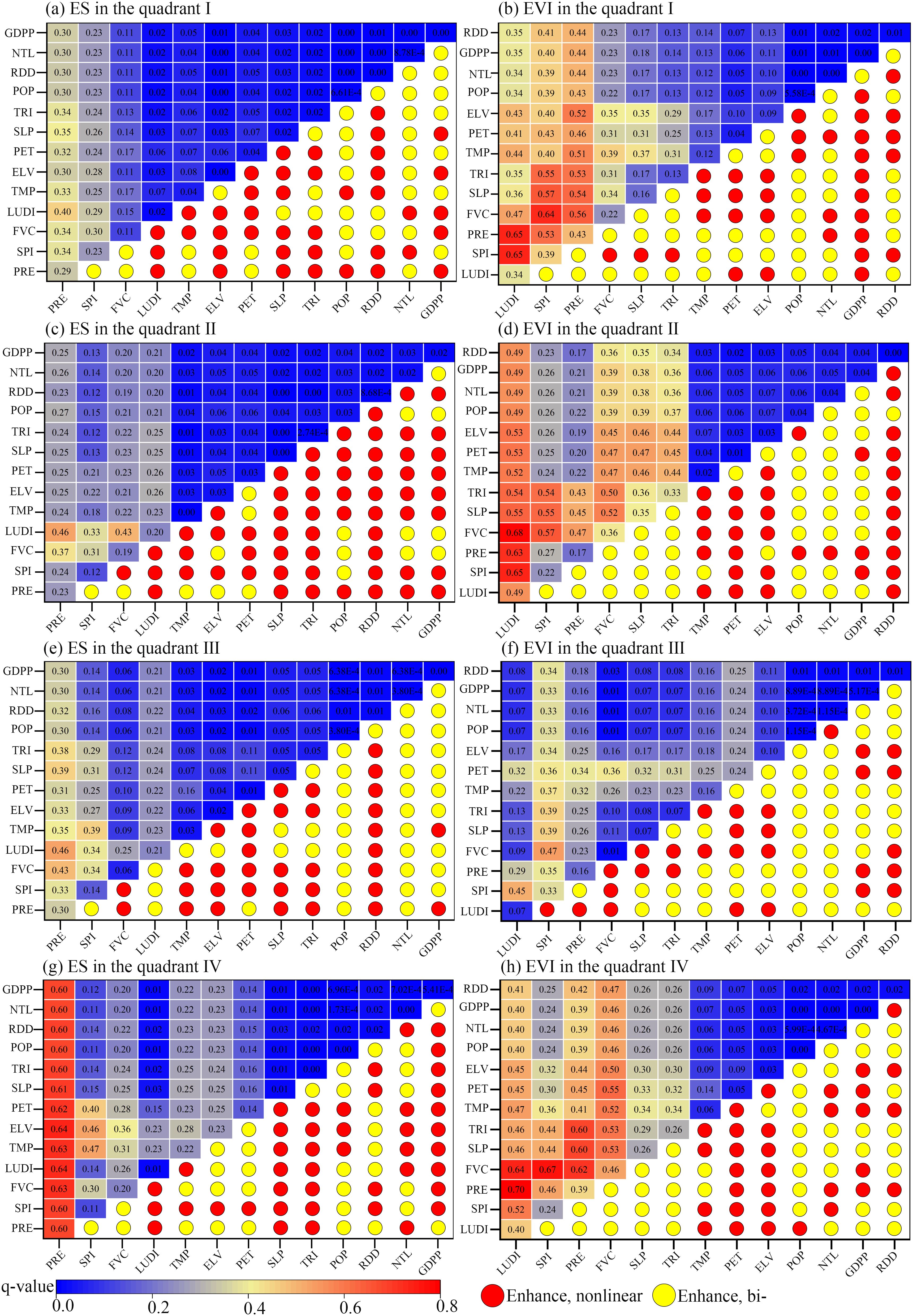
Figure 11. Interaction of driving factors on ES and EVI in each quadrant.

Figure 11 displays the interaction explanatory power of 13 driving factors on ES and EVI spatial distribution patterns. In the ZC area, the types of factor interactions were limited to bi-factor enhancement (Enhance, bi-) and nonlinear enhancement (Enhance, nonlinear), indicating that the combined effects of two factors were stronger than their individual effects. In Quadrant I, the strongest interactions for ES were PRE∩LUDI (0.40), PRE∩SLP (0.35), and PRE∩FVC (0.34), while the strongest interactions for EVI were LUDI∩SPI (0.65), LUDI∩PRE (0.65), and SPI∩FVC (0.64) (Figures 11a, b). In Quadrant II, the strongest interactions for ES were PRE∩LUDI (0.46), FVC∩LUDI (0.43), and PRE∩FVC (0.37), while the strongest interactions for EVI were LUDI∩FVC (0.68), LUDI∩SPI (0.65), and LUDI∩PRE (0.63) (Figures 11c, d). In Quadrant III, the strongest interactions for ES were PRE∩LUDI (0.46), PRE∩FVC (0.46), and PRE∩SLP (0.39), while the strongest interactions for EVI were SPI∩FVC (0.47), LUDI∩SPI (0.45), and SPI∩SLP (0.39) (Figures 11e, f). In Quadrant IV, the strongest interactions for ES were PRE∩LUDI (0.64), PRE∩ELV (0.64), and PRE∩FVC (0.63), while the strongest interactions for EVI were LUDI∩PRE (0.70), SPI∩FVC (0.67), and LUDI∩FVC (0.64) (Figures 11g, h).

4 Discussion

4.1 Spatiotemporal changes of ES and EVI in the ZC area

The ZC area plays a crucial role as an ecological barrier in the Beijing–Tianjin–Hebei (BTH) region, and the assessment of its ecosystem services (ES) and ecological vulnerability (EVI) is essential for understanding regional ecological security. Our findings reveal that from 2000 to 2020, ES increased while EVI declined, with the most pronounced changes occurring between 2000 and 2010. These trends are consistent with broader regional studies covering the BTH area, which includes the ZC region (Fu and Liu, 2024; Gong et al., 2024). Previous studies have similarly attributed ecological improvements to large-scale ecological restoration programs such as afforestation, water source conservation forests, and integrated ecological engineering (Yang et al., 2019). Our analysis confirms these findings and further quantifies the spatiotemporal interactions between ES and EVI using a combined Z-score classification and GeoDetector analysis. Compared to earlier studies that often assessed ES or EVI independently, our integrative approach offers a more comprehensive understanding of ecological dynamics. However, after 2010, we observed a slowdown in ES improvement and a plateau in EVI reduction, likely due to increasing anthropogenic pressures associated with urbanization and energy consumption (Chu et al., 2017). This pattern highlights the limitations of passive restoration when not accompanied by sustainable development strategies.

The spatial distribution of ES and EVI indicate that WY, SC, and CS showed an increasing trend from west to east, while FS and EVI showed a decreasing trend from west to east. These patterns are consistent with prior studies (Gong et al., 2024). The western regions, which belong to a semi-arid climate zone, are characterized by poor vegetation conditions, severe soil erosion, and high sensitivity to external disturbances such as climate change (e.g., droughts) and human activities (e.g., overexploitation and grazing) (Jiang et al., 2021). Consequently, the overall ecosystem is more fragile. In contrast, the central and eastern regions, which experience higher precipitation, better vegetation cover, and weaker soil erosion, show lower levels of ecological vulnerability.

The synergistic relationships between WY, SC, and CS can be explained by the favorable water and heat conditions in the central and eastern regions, which promote vegetation development, enhance soil erosion resistance, and increase the region’s carbon sequestration ability, thus reducing EVI (Zhou et al., 2021). However, FS exhibited trade-offs with other ES, mainly due to intense human agricultural activities in the western regions, which alter soil structure, destroy natural vegetation, and inhibit positive ecological succession. As a result, FS is high, leading to a higher EVI in these regions. This indicates that the common or dominant factors of different ES play a significant role in shaping the complex spatial relationship with EVI. Exploring how different ecosystem service trade-offs and synergies impact EVI will be an important research direction.

4.2 Spatial distribution patterns of ES and EVI based on Z-score normalization

Traditional analyses of the spatial distribution of ES or EVI often rely on raw values for quantitative interpretation. However, this approach can be affected by variations in data scales, regional climate conditions, and land-use patterns, potentially leading to biased or misleading conclusions. To address these limitations, this study employs Z-score normalization to analyze the spatial patterns of ES and EVI. Z-score normalization converts raw data into dimensionless standardized values, thereby eliminating differences in scale and enabling direct comparison of ES and EVI across diverse regions. This method enhances the clarity of spatial distribution patterns and reduces analytical bias caused by heterogeneous data characteristics (Tarasewicz and Jönsson, 2021). Moreover, normalized data more effectively highlight variations in ecosystem service functions and ecological vulnerability, making it a powerful and intuitive tool for spatial analysis, especially in ecologically complex areas with diverse geographical and climatic conditions.

By standardizing the data with Z-scores, we integrated the ES and EVI values into a comprehensive framework and examined their spatial distribution patterns across different quadrants. Quadrant I (High ES, High EVI): Typical regions include the central mountainous areas and regions with good forest cover, where significant ecological services in terms of WY, SC, and CS are provided. However, due to climate change and human activity, the EVI in these areas is relatively high. Therefore, effective ecological protection measures are required to prevent further ecological degradation. Quadrant II (Low ES, High EVI): These regions are mainly found in arid or semi-arid areas, where the terrain and climate conditions limit the level of ES. These areas have high ecological restoration potential and require restoration and conservation efforts to reduce ecological vulnerability. Quadrant III (Low ES, Low EVI): These regions, mainly in the western areas with excessive agricultural development and serious land degradation, exhibit high FS but weakened WY, SC, and CS due to over-cultivation and grassland reclamation. As a result, ecological vulnerability increases, and the region requires stronger land restoration and the promotion of sustainable agricultural practices to reduce land degradation and restore ES. Quadrant IV (High ES, Low EVI): These areas, due to effective ecological protection measures and sustainable resource management, avoid over-exploitation and excessive resource use. With proper water resource management and protection, the ecosystems maintain high stability, reducing the risk of ecological vulnerability. These areas need to continue maintaining strong ecological protection measures to ensure long-term stability of their ecological functions.

A point worth further discussion is that although ES and EVI are theoretically expected to have a negative correlation, in some regions, there may be reverse or complex interactions between the two (Liu et al., 2020). In rapidly developing areas, despite abundant ecological services (e.g., FS and WY), human activities may lead to increased EVI. This phenomenon is common in agricultural zones and areas surrounding urban centers, where large amounts of food and water resources are provided, but the long-term stability and sustainability of the ecosystem are at risk. Therefore, the relationship between ES and EVI is not always a simple positive or negative correlation, but may exhibit different complex relationships depending on the region and environmental conditions (Metzger et al., 2008). This presents an important research direction: how to enhance ES while mitigating or avoiding an increase in EVI, in order to balance ecological protection with human needs.

4.3 Effects of driving factors on the spatial distribution of ES and EVI

In the ZC area, climatic factors play a critical role in shaping the spatial distribution of ES and EVI. In regions with abundant precipitation—particularly mountainous areas with dense forest cover—the combination of high PRE and TMP promotes WY and SC, thereby enhancing overall ES. In contrast, arid regions with limited precipitation experience reduced WY, which negatively affects ES, especially WY and CS. These drier areas also tend to exhibit higher EVI due to lower ecological resilience. In addition to climatic influences, LUDI, including agricultural expansion and urbanization, significantly impact ES and EVI in the ZC area. The conversion of natural land into cropland or urban areas has led to decreased FVC and increased soil erosion, resulting in the degradation of ES. Furthermore, intensified land-use activities have contributed to rising EVI by exerting greater pressure on already fragile ecosystems (Sun et al., 2020).

The interaction of factors has a more complex and significant effect on ES and EVI. Interactions among multiple factors can amplify their individual effects. For example, the interaction between climate and land-use changes in the ZC area has generally led to negative effects. In areas with low PRE, the interaction of land-use changes and climate factors has exacerbated WY reduction. In Quadrant I (High ES, High EVI), favorable climatic conditions—particularly adequate precipitation and temperature—combined with high fractional vegetation cover (FVC), have jointly promoted improvements in water yield (WY), soil conservation (SC), and carbon sequestration (CS). These areas are typically mountainous regions with dense forest cover, where the interaction between precipitation (PRE) and FVC contributes to enhanced ES stability. Despite high ES, ecological vulnerability remains elevated due to natural fragility. The influence of land use intensity (LUDI) is relatively limited in these zones, which are often located within nature reserves or well-preserved ecological areas. In Quadrant II (Low ES, High EVI), the interaction between adverse climatic factors and intensive land-use changes is more pronounced. Low precipitation and high LUDI—resulting from over-cultivation, overgrazing, and other anthropogenic disturbances—have led to severe water shortages and accelerated soil erosion. These processes significantly reduce ES, particularly WY and SC, and exacerbate ecological vulnerability. The compounded effects of these interacting factors make ecological restoration particularly difficult in these areas. In Quadrant III (Low ES, Low EVI), arid and semi-arid environmental conditions dominate. Low PRE, degraded soils, and intensive land use contribute to reduced ES and, paradoxically, relatively low EVI. However, the interaction of these factors still produces negative outcomes: persistent drought stress coupled with inappropriate land management leads to ongoing ecosystem degradation and latent ecological risk. In Quadrant IV (High ES, Low EVI), the interaction between favorable climatic conditions and relatively sustainable land use plays a positive role. These regions are characterized by high ES and low ecological vulnerability, benefiting from increased FVC and optimized land-use structures. However, in some localized areas, the effects of land-use changes—such as insufficient control of soil erosion—still present challenges. While the overall interaction of drivers enhances ES, it also reveals certain residual vulnerabilities that warrant continued ecological monitoring and management.

Interactions between driving factors in the ZC area generally exhibit an enhancement effect. In areas with intense human activity, such as agricultural land and rapidly urbanizing zones, the interaction between land-use changes and climate change has further decreased ES and increased EVI. Specifically, the combined effect of drought and land-use changes has led to a significant decline in WY, and the decrease in SC and CS has intensified the rise in EVI. Conversely, in areas with more moderate climates and higher FVC, the interaction of factors has positively influenced ES, enhanced ecosystem stability, and mitigated the trend of increasing EVI.

5 Conclusion

Based on the assessment of ES and EVI in the ZC area, this study explores the spatiotemporal changes, correlations, and spatial distribution patterns of ES and EVI, and further analyzes the effects of various driving factors. The major findings are listed as follows: (1) ES increased by 46.3%, while EVI decreased by 12.5%. The most significant changes occurred between 2000 and 2010, with the most significant changes occurring between 2000 and 2010. (2) The spatial distribution of ES and EVI, based on Z-score normalization, shows clear patterns. Quadrant I (High ES, High EVI) features areas with strong ecosystem services but high vulnerability. Quadrant II (Low ES, High EVI) includes regions with both low ecosystem services and high ecological vulnerability. Quadrant III (Low ES, Low EVI) represents degraded areas with low ecosystem services and vulnerability. Quadrant IV (High ES, Low EVI) includes areas with high ecosystem services and low vulnerability, benefiting from effective management. (3) Meteorological and land-use interactions significantly influence ES and EVI. In areas with favorable meteorological conditions and high vegetation cover, these interactions enhance ES and reduce EVI. In contrast, in arid regions with intense human activity, they exacerbate ecological degradation, decreasing ES and increasing EVI. These findings offer critical insights for informing policy decisions related to ecological conservation, land management, and sustainable development in ecologically vulnerable regions.

Data availability statement

The original contributions presented in the study are included in the article/supplementary material. Further inquiries can be directed to the corresponding author.

Author contributions

YW: Conceptualization, Data curation, Formal analysis, Funding acquisition, Investigation, Methodology, Project administration, Resources, Software, Supervision, Validation, Visualization, Writing – original draft, Writing – review & editing. ZX: Writing – review & editing. AJ: Data curation, Writing – review & editing. YY: Data curation, Writing – review & editing. WR: Data curation, Writing – review & editing. CW: Conceptualization, Data curation, Writing – review & editing.

Funding

The author(s) declare that financial support was received for the research and/or publication of this article. This work was supported by Hebei Key Laboratory of Mountain Geological Environment (grant numbers: HBKLMGE202403); Higher Education Science and Technology Research Project for Hebei Province (grant numbers: BJK2023105); Youth Fund Project for Hebei Minzu Normal University (grant numbers: QN2024002); Youth Fund Project for Hebei Minzu Normal University (grant numbers: QN2020002); Science and Technology Special Project for the Construction of the Chengde National Sustainable Development Agenda Innovation Demonstration Area (grant numbers: 202302F006); Team Development Fund Project for University-level Scientific Research, Hebei Minzu Normal University(grant numbers: TD2024002).

Acknowledgments

The authors are grateful to the editor and reviewers for their careful and valuable suggestions.

Conflict of interest

The authors declare that the research was conducted in the absence of any commercial or financial relationships that could be construed as a potential conflict of interest.

Generative AI statement

The author(s) declare that no Generative AI was used in the creation of this manuscript.

Publisher’s note

All claims expressed in this article are solely those of the authors and do not necessarily represent those of their affiliated organizations, or those of the publisher, the editors and the reviewers. Any product that may be evaluated in this article, or claim that may be made by its manufacturer, is not guaranteed or endorsed by the publisher.

References

Abson D. J., Dougill A. J., and Stringer L. C. (2012). Using Principal Component Analysis for information-rich socio-ecological vulnerability mapping in Southern Africa. Appl. Geography. 35, 515–524. doi: 10.1016/j.apgeog.2012.08.004

Crossref Full Text | Google Scholar

Adger W. N. (2006). Vulnerability. Global Environ. Change-Human Policy Dimensions. 16, 268–281. doi: 10.1016/j.gloenvcha.2006.02.006

Crossref Full Text | Google Scholar

Chu X., Deng X. Z., Jin G., Wang Z., and Li Z. H. (2017). Ecological security assessment based on ecological footprint approach in Beijing-Tianjin-Hebei region, China. Phys. Chem. Earth. 101, 43–51. doi: 10.1016/j.pce.2017.05.001

Crossref Full Text | Google Scholar

Costanza R., dArge R., deGroot R., Farber S., Grasso M., Hannon B., et al. (1997). The value of the world’s ecosystem services and natural capital. Nature. 387, 253–260. doi: 10.1038/387253a0

Crossref Full Text | Google Scholar

Costanza R., de Groot R., Sutton P., van der Ploeg S., Anderson S. J., Kubiszewski I., et al. (2014). Changes in the global value of ecosystem services. Global Environ. Change-Human Policy Dimensions. 26, 152–158. doi: 10.1016/j.gloenvcha.2014.04.002

Crossref Full Text | Google Scholar

Deng C. X., Liu J. Y., Liu Y. J., Li Z. W., Nie X. D., Hu X. Q., et al. (2021). Spatiotemporal dislocation of urbanization and ecological construction increased the ecosystem service supply and demand imbalance. J. Environ. Management. 288, 112478. doi: 10.1016/j.jenvman.2021.112478

PubMed Abstract | Crossref Full Text | Google Scholar

Eniyew S., Teshome M., Sisay E., and Bezabih T. (2021). Integrating RUSLE model with remote sensing and GIS for evaluation soil erosion in Telkwonz Watershed, Northwestern Ethiopia. Remote Sens. Applications-Society And Environment. 24, 100623. doi: 10.1016/j.rsase.2021.100623

Crossref Full Text | Google Scholar

Fu X. Y. and Liu Y. J. (2024). Ecological vulnerability assessment and spatiotemporal characteristics analysis of urban green-space systems in beijing-tianjin-hebei region. Sustainability. 16, 1–22. doi: 10.3390/su16062289

Crossref Full Text | Google Scholar

Gao J. B., Jiao K. W., and Wu S. H. (2018). Quantitative assessment of ecosystem vulnerability to climate change: methodology and application in China. Environ. Res. Letters. 13, 094016. doi: 10.1088/1748-9326/aadd2e

Crossref Full Text | Google Scholar

Gong S. X., Zhang Y. H., Pu X., Wang X. H., Zhuang Q. Y., and Bai W. H. (2024). Assessing and predicting ecosystem services and their trade-offs/synergies based on land use change in beijing-tianjin-hebei region. Sustainability. 16, 1–22. doi: 10.3390/su16135609

Crossref Full Text | Google Scholar

Gu H. L., Huan C. Y., and Yang F. J. (2023). Spatiotemporal dynamics of ecological vulnerability and its influencing factors in shenyang city of China: based on SRP model. Int. J. Environ. Res. Public Health 20, 1525. doi: 10.3390/ijerph20021525

PubMed Abstract | Crossref Full Text | Google Scholar

He L., Shen J., and Zhang Y. (2018). Ecological vulnerability assessment for ecological conservation and environmental management. J. Environ. Management. 206, 1115–1125. doi: 10.1016/j.jenvman.2017.11.059

PubMed Abstract | Crossref Full Text | Google Scholar

Jiang M. C., He Y. X., Song C. H., Pan Y. P., Qiu T., and Tian S. F. (2021). Disaggregating climatic and anthropogenic influences on vegetation changes in Beijing-Tianjin-Hebei region of China. Sci. Total Environment. 786, 147574. doi: 10.1016/j.scitotenv.2021.147574

Crossref Full Text | Google Scholar

Jiang C., Li D. Q., Wang D. W., and Zhang L. B. (2016). Quantification and assessment of changes in ecosystem service in the Three-River Headwaters Region, China as a result of climate variability and land cover change. Ecol. Indicators. 66, 199–211. doi: 10.1016/j.ecolind.2016.01.051

Crossref Full Text | Google Scholar

Liu Y. M., Yang S. N., Han C. L., Ni W., and Zhu Y. Y. (2020). Variability in regional ecological vulnerability: A case study of sichuan province, China. Int. J. Disaster Risk Science. 11, 696–708. doi: 10.1007/s13753-020-00295-6

Crossref Full Text | Google Scholar

Ma S., Qiao Y. P., Wang L. J., and Zhang J. C. (2021). Terrain gradient variations in ecosystem services of different vegetation types in mountainous regions: Vegetation resource conservation and sustainable development. For. Ecol. Management. 482, 118856. doi: 10.1016/j.foreco.2020.118856

Crossref Full Text | Google Scholar

Malekmohammadi B. and Jahanishakib F. (2017). Vulnerability assessment of wetland landscape ecosystem services using driver-pressure-state-impact-response (DPSIR) model. Ecol. Indicators. 82, 293–303. doi: 10.1016/j.ecolind.2017.06.060

Crossref Full Text | Google Scholar

Metzger M. J., Schröter D., Leemans R., and Cramer W. (2008). A spatially explicit and quantitative vulnerability assessment of ecosystem service change in Europe. Regional Environ. Change. 8, 91–107. doi: 10.1007/s10113-008-0044-x

Crossref Full Text | Google Scholar

Mumby P. J., Chollett I., Bozec Y. M., and Wolff N. H. (2014). Ecological resilience, robustness and vulnerability: how do these concepts benefit ecosystem management? Curr. Opin. Environ. Sustainability. 7, 22–27. doi: 10.1016/j.cosust.2013.11.021

Crossref Full Text | Google Scholar

Qiu B. K., Li H. L., Zhou M., and Zhang L. (2015). Vulnerability of ecosystem services provisioning to urbanization: A case of China. Ecol. Indicators. 57, 505–513. doi: 10.1016/j.ecolind.2015.04.025

Crossref Full Text | Google Scholar

Raheem N., Cravens A. E., Cross M. S., Crausbay S., Ramirez A., McEvoy J., et al. (2019). Planning for ecological drought: Integrating ecosystem services and vulnerability assessment. Wiley Interdiscip. Reviews-Water. 6, e1352. doi: 10.1002/wat2.2019.6.issue-4

Crossref Full Text | Google Scholar

Shoyama K. and Yamagata Y. (2014). Predicting land-use change for biodiversity conservation and climate-change mitigation and its effect on ecosystem services in a watershed in Japan. Ecosystem Services. 8, 25–34. doi: 10.1016/j.ecoser.2014.02.004

Crossref Full Text | Google Scholar

Sun T., Yang L., Sun R. H., and Chen L. D. (2020). Key factors shaping the interactions between environment and cities in megalopolis area of north China. Ecol. Indicators. 109, 105771. doi: 10.1016/j.ecolind.2019.105771

Crossref Full Text | Google Scholar

Tang Q., Wang J. M., and Jing Z. R. (2021). Tempo-spatial changes of ecological vulnerability in resource-based urban based on genetic projection pursuit model. Ecol. Indicators. 121, 107059. doi: 10.1016/j.ecolind.2020.107059

Crossref Full Text | Google Scholar

Tarasewicz N. A. and Jönsson A. M. (2021). An ecosystem model based composite indicator, representing sustainability aspects for comparison of forest management strategies. Ecol. Indicators. 133, 108456. doi: 10.1016/j.ecolind.2021.108456

Crossref Full Text | Google Scholar

Vargas L., Willemen L., and Hein L. (2019). Assessing the capacity of ecosystems to supply ecosystem services using remote sensing and an ecosystem accounting approach. Environ. Management. 63, 1–15. doi: 10.1007/s00267-018-1110-x

PubMed Abstract | Crossref Full Text | Google Scholar

Wang S. J., Liu Z. T., Chen Y. X., and Fang C. L. (2021). Factors influencing ecosystem services in the Pearl River Delta, China: Spatiotemporal differentiation and varying importance. Resour. Conserv. Recycling. 168, 105477. doi: 10.1016/j.resconrec.2021.105477

Crossref Full Text | Google Scholar

Wang X. Z., Wu J. Z., Liu Y. L., Hai X. Y., Shanguan Z. P., and Deng L. (2022). Driving factors of ecosystem services and their spatiotemporal change assessment based on land use types in the Loess Plateau. J. Environ. Management. 311, 1–22. doi: 10.1016/j.jenvman.2022.114835

PubMed Abstract | Crossref Full Text | Google Scholar

Wang C., Zhan J. Y., Chu X., Liu W., and Zhang F. (2019). Variation in ecosystem services with rapid urbanization: A study of carbon sequestration in the Beijing-Tianjin-Hebei region, China. Phys. Chem. Earth. 110, 195–202. doi: 10.1016/j.pce.2018.09.001

Crossref Full Text | Google Scholar

Weisshuhn P., Müller F., and Wiggering H. (2018). Ecosystem vulnerability review: proposal of an interdisciplinary ecosystem assessment approach. Environ. Management. 61, 904–915. doi: 10.1007/s00267-018-1023-8

PubMed Abstract | Crossref Full Text | Google Scholar

Xie Z. L., Li X. Z., Chi Y., Jiang D. G., Zhang Y. Q., Ma Y. X., et al. (2021). Ecosystem service value decreases more rapidly under the dual pressures of land use change and ecological vulnerability: A case study in Zhujiajian Island. Ocean Coast. Management. 201, 105493. doi: 10.1016/j.ocecoaman.2020.105493

Crossref Full Text | Google Scholar

Yang X., Chen R. S., Meadows M. E., Ji G. X., and Xu J. H. (2020). Modelling water yield with the InVEST model in a data scarce region of northwest China. Water Supply. 20, 1035–1045. doi: 10.2166/ws.2020.026

Crossref Full Text | Google Scholar

Yang H. F., Zhai G. F., and Zhang Y. (2021). Ecological vulnerability assessment and spatial pattern optimization of resource-based cities: A case study of Huaibei City, China. Hum. Ecol. Risk Assessment. 27, 606–625. doi: 10.1080/10807039.2020.1744426

Crossref Full Text | Google Scholar

Yang Y. Y., Zheng H., Xu W. H., Zhang L., and Ouyang Z. Y. (2019). Temporal changes in multiple ecosystem services and their bundles responding to urbanization and ecological restoration in the beijing-tianjin-hebei metropolitan area. Sustainability. 11, 2079. doi: 10.3390/su11072079

Crossref Full Text | Google Scholar

Zeng X. T., Zhao J. Y., Wang D. Q., Kong X. M., Zhu Y., Liu Z. P., et al. (2019). Scenario analysis of a sustainable water-food nexus optimization with consideration of population-economy regulation in Beijing-Tianjin-Hebei region. J. Of Cleaner Production. 228, 927–940. doi: 10.1016/j.jclepro.2019.04.319

Crossref Full Text | Google Scholar

Zhang M. M., Kafy A. A., Ren B., Zhang Y. W., Tan S. K., and Li J. X. (2022). Application of the optimal parameter geographic detector model in the identification of influencing factors of ecological quality in guangzhou, China. Land. 11, 1–22. doi: 10.3390/land11081303

Crossref Full Text | Google Scholar

Zhang W. W. and Li H. (2016). Characterizing and assessing the agricultural land use intensity of the beijing mountainous region. Sustainability. 8, 1180. doi: 10.3390/su8111180

Crossref Full Text | Google Scholar

Zhang S. and Liu L. Y. (2014). The potential of the MERIS Terrestrial Chlorophyll Index for crop yield prediction. Remote Sens. Letters. 5, 733–742. doi: 10.1080/2150704X.2014.963734

Crossref Full Text | Google Scholar

Zhao M. M., He Z. B., Du J., Chen L. F., Lin P. F., and Fang S. (2019). Assessing the effects of ecological engineering on carbon storage by linking the CA-Markov and InVEST models. Ecol. Indicators. 98, 29–38. doi: 10.1016/j.ecolind.2018.10.052

Crossref Full Text | Google Scholar

Zhou Y. Y., Fu D. J., Lu C. X., Xu X. M., and Tang Q. H. (2021). Positive effects of ecological restoration policies on the vegetation dynamics in a typical ecologically vulnerable area of China. Ecol. Engineering. 159, 106087. doi: 10.1016/j.ecoleng.2020.106087

Crossref Full Text | Google Scholar

Zhou W., Xi Y. T., Zhai L., Li C., Li J. Y., and Hou W. (2023a). Zoning for spatial conservation and restoration based on ecosystem services in highly urbanized region: A case study in beijing-tianjin-hebei, China. Land. 12, 733. doi: 10.3390/land12040733

Crossref Full Text | Google Scholar

Zou T. H., Chang Y. X., Chen P., and Liu J. F. (2021). Spatial-temporal variations of ecological vulnerability in Jilin Province (China), 2000 to 2018. Ecol. Indicators. 133, 108429. doi: 10.1016/j.ecolind.2021.108429

Crossref Full Text | Google Scholar