 Daniel J. Silva
 João S. Amaral
 Vitor S. Amaral
- Department of Physics and CICECO - Aveiro Institute of Materials, University of Aveiro, Aveiro, Portugal
Prototyping innovative energy devices is a complex multivariable dimensioning problem. For the case of magnetocaloric systems, one aims to obtain an optimized balance between energy conversion performance, useful power generated, and power consumed. In these devices, modeling is entering a mature phase, but dimensioning is still time consuming. We have developed a technique that dimensions any type of magnetocaloric system by training statistical learning classifiers that are used to simulate the computation of a very large number of systems with different combinations of parameters to be dimensioned. We used this method in the dimensioning of a magnetocaloric heat pump aiming at optimizing the temperature span, heating power, and coefficient of performance, obtaining an f-score of 95%. The respective classifier was used to mimic over 940 thousand computed systems. The gain in computation time was 300 times that of computing numerically the system for each combination of parameters.
1. Introduction
One of the goals of the 2030 United Nations agenda for sustainable development is to “ensure access to affordable, reliable, sustainable and modern energy for all.” One way for energy consumption to become more sustainable is to increase the energy efficiency of common household devices, such as water heaters. In this context, magnetocaloric systems have been pointed out as a reliable alternative to vapor compression technology for heat pumps and refrigerators (Gschneidner and Pecharsky, 2008; Yu et al., 2010; Kitanovski et al., 2015a). In fact, the coefficient of performance (COP) can attain high values when compared to the vapor compression systems (Yu et al., 2003). Magnetocaloric systems rely on magnetizing and demagnetizing magnetocaloric materials (MCM) for creating temperature gradients instead of compressing and expanding gases (Tishin and Spichkin, 2003; Kitanovski et al., 2015b). Therefore, the magnetocaloric technology does not require the use of nocive gases. One important breakthrough that increased the research on the development of new magnetocaloric systems was the use of the active magnetic regenerative cycle, where the magnetocaloric material acts as both the refrigerant and regenerator (Barclay and Steyert, 1982). This cycle allowed to increase the potential temperature span several times.
Because the regenerator is the core element of magnetocaloric systems, their thermal properties (Franco et al., 2012; Moya et al., 2014; Lyubina, 2017) and geometries are of paramount importance. In that respect, several geometries have been considered (Nielsen et al., 2013; Lei et al., 2017). In particular, parallel plates regenerators and packed spheres have been pointed out as the most practical designs (Engelbrecht et al., 2013; Tušek et al., 2013; Aprea et al., 2017; Trevizoli et al., 2017). Although such designs show some level of simplicity, several parameters must be dimensioned. In that respect, several works aiming the dimensioning of prototypes have been performed. Li et al. (2008) optimized an active magnetic regenerative refrigerator with a second-law analysis. Nielsen et al. (2010) investigated the influence of the plate and channel thickness, cycle frequency and fluid motion on the performance of a magnetocaloric refrigerator. Roudaut et al. (2011) analyzed the implication of several parameters on the number of units, utilization factor, and axial conductivity. Li et al. (2012) dimensioned an active magnetic refrigerator by using an analytical model. Tagliafico et al. (2012) performed a parametric investigation on the frequency and fluid mass flow rate. The same authors, along with Aprea et al., used dimensioned models for the optimization (Aprea et al., 2013; Tagliafico et al., 2013). Risser et al. (2013) improved a numerical model aiming the optimization of the design of a magnetocaloric refrigerators. Trevizoli et al. (2014) and Trevizoli et al. (2016) included thermomagnetic phenomena and losses in their numerical model. Moreover, the same authors identified the most appropriate parameters and operating conditions following an entropy generation minimization analysis of active magnetic regenerators (Trevizoli and Barbosa, 2017). Bouchekara et al. (2014) created a multiobjective optimization model. Niknia et al. (2016) included configuration losses in their parametric study. Finally, Roy et al. (2017) used a genetic algorithm in their multiobjective optimization model. Although these parametric investigations achieved the goal of dimensioning magnetocaloric systems, the development of a complete and reliable systematic dimensioning technique has been hindered by the computational cost of performing brute force computation, i.e., of systematically performing the numerical computation of systems with a large number of combinations of parameters to be dimensioned. For instance, for only 7 parameters, and only considering 10 different values for each one, it would be necessary to compute ten million different systems to figure out which values fulfills the requirements.
One way to reduce the number of computed systems for dimensioning procedures is by predicting, through statistical learning classifiers, the outcome of a dimensioned system, if such a method is computationally more efficient assuming trustworthy predictions. Generally speaking, statistical learning classifiers have recently been used in solving several problems in Physics, e.g., in predicting non-linear theories for multiscale modeling of heterogeneous materials (Matouš et al., 2017), in proposing strategies for systems with invariance properties (Ling et al., 2016), or in guiding the creation of improved closure models for computational physics applications (Parish and Duraisamy, 2016). In this work we present a new method for dimensioning magnetocaloric systems. We exemplify the method for a reciprocating heat pump with parallel plates regenerators. We optimize the method by testing with the statistical learning classifiers K-nearest neighbors (KNN), multilayer Perceptron (MLP), support vector machines (SVM), and random forests (RF). The performance of the method is showed for the temperature span, heating power and COP.
2. Magnetocaloric Model
The full process of obtaining the dataset by using the heatrapy python framework is described in this section (hea, 2018). The modeled system is unidimensional and is described in Silva et al. (2018) for hydraulic active magnetic regenerative systems. As depicted in Figure 1, it consists of four elements: one fluid, one MCM, one hot heat exchanger (HHEX), and one cold heat exchanger (CHEX). One should note that this process can easily be substitute by other numerical algorithms, e.g. by using other commercial softwares with similar numerical approaches.
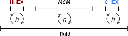
Figure 1. Geometry for the unidimensional active magnetic refrigerator model. The fluid is static, while the MCM, hot and cold heat exchangers (HHEX and CHEX, respectively) moves cyclically in the horizontal direction. Heat is transferred between the fluid and the 3 remaining elements (h).
2.1. Governing Equations and Boundary Conditions
The governing equations are the following (Petersen et al., 2008a,b; Nielsen et al., 2009, 2011; Aprea and Maiorino, 2010; Lienhard, 2017):
where T is the temperature, x the position, t the time, ρ the density of the material, CH the specific heat at constant H, k the thermal conductivity, V the velocity of the fluid, and the subscript s and f defines the type of material, solid or fluid, respectively. Qsf is the heat transfer power per volume between the solids and fluid. In the present model one considers the fluid framework so that the fluid is static (V = 0) and the other three components are moving forward and backward as shown in Figure 1. In this context, the convective term of Equation (2) vanishes and the overall problem is reduced to a heat conduction problem. The equations were solved by using the Crank-Nicholsen implicit finite difference method with the “implicit_k(x)” solver of the heatrapy package (Silva et al., 2018):
where i and n stand for the space and time index, Δx and Δt stand for the space and time steps respectively and .The used Δx and Δt were 0.001 m and 0.01 s, respectively. Note that the heatrapy package was validated for magnetocaloric fluidic systems (Silva et al., 2019b).
The magnetocaloric effect was considered by using a temperature step change (Silva et al., 2018):
where - and + stand for the removal and application of H, so that and account for the adiabatic temperature change when applying and removing H, respectively. The and curves were obtained with the specific heat CH(T) curves for H=0 and H=1T, which were calculated with the Weiss, Debye and Sommerfeld models for Gd (Petersen et al., 2008b; Silva et al., 2018).
To obtain temperature span values, and since this work exemplifies magnetocaloric systems with the case of heat pumps, insulation was imposed for the HHEX, and the CHEX was kept at a fixed operating temperature. On the other hand, to obtain heating power quantities the temperature of both reservoirs were kept at fixed values. The fixed temperature boundary conditions were modeled by keeping constant the temperature of the boundary point:
where b is the boundary position. Thermal insulation is modeled by keeping the temperature of the previous point equal to the boundary point:
For more information about the implementation of these conditions consult (Silva et al., 2012, 2014, 2016, 2019a,c).
2.2. Used Materials and Parameters to Be Dimensioned
The used values for CH, ΔTad, ρ, and k for Gd were extracted from Petersen et al. (2008b). While CH and ΔTad is strongly dependent on temperature, ρ and k can be considered as being fixed at 7,900 Kg/m3 and 10.5 W/(mK). Water was chosen for the fluid and copper for both the heat exchangers (HEXs). All the physical properties of the used materials in the modeled system are listed in Table 1.
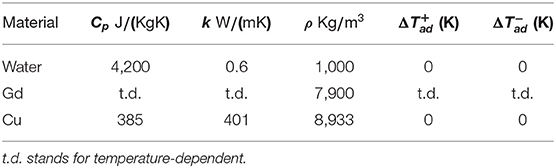
Table 1. Physical properties of the used materials in the modeled system (mat, 2019).
Seven different parameters were considered in the dimensioning of the magnetocaloric heat pump, and are the inputs of each performed simulation:
1. Operating frequency of the heat pump (ν), with values ranging from 0.01 to 4.51 Hz.
2. Thickness of each parallel plate (ϵ), with values ranging from 0.5 to 2.5 mm.
3. Distance between parallel plates (dp−p), with values ranging from 0.5 to 2.5 mm.
4. MCM axial length (lMCM), with values ranging from 1 to 10 cm.
5. HEX axial length (lHEX), with values ranging from 1 to 10 cm.
6. Distance between the MCM and heat exchangers (d), with values ranging from 1 to 10 cm.
7. Stroke of the water pump, or motion amplitude of the fluid (s), with values ranging from 1 to 10 cm.
2.3. Performance Variables
In the present investigation three performance variables were considered: the temperature span of the heat pump, heating power, and COP.
The temperature span of a magnetocaloric heat pump ΔT is the temperature difference between the HHEX (Thot) and CHEX (Tcold) when the CHEX is at a fixed temperature and the HHEX is insulated:
These values are calculated when attaining the stationary state criteria, which in the present case occurs when the temperature change between two consecutive cycles is less than 10−6.
The heating power per sectional area (Pheat) is the energy per time and area that, within one cycle in the stationary state, the system is pumping to the HHEX. To obtain this value one must fix both temperatures splitted below the no load temperature span. In the present case the zero temperature span condition was chosen, i.e., both HEX were fixed at the same temperature (ambient temperature).
One of the most important performance quantities is the COP of a magnetocaloric system, which relates the energy needed, in the form of work, to pump a useful quantity of heat within one cycle. For the case of heat pumps it follows the formula:
where Pwork is the average power per sectional area within a cycle in the stationary state required to pump the heat from the cold to the hot reservoirs. This power can be approximated by
where smax and νmax are the maximum stroke and maximum operating frequency considered, i.e., 10 cm and 4.51 Hz, respectively. Pmax is the total maximum power that need to be given to the motor that moves the magnets and to the water pump. Most of the losses are indirectly incorporated in Equation (9), e.g., viscous losses. In the present case it was considered Pmax=5 × 10⁶ Wm−2, which was the value to obtain a COP=3 for zero temperature span when using a frequency of 0.5 Hz and stroke of 2 cm. Note that, e.g., a Pwork of 106 Wm−2 means that a regenerator with a cross section of 1m2 will require 106 W of working power. A more realistic regenerator of 2cm2, with the same Pwork, will require 200W of working power.
2.4. Dataset
The obtained dataset was extracted from 3,000 simulations, each one considering random values with a uniform distribution of the 7 input variables, known in statistic learning as predictors. The computation time for the 3,000 simulations was 2 months using 25 cores (Intel(R) Xeon(R) CPU E5-2690 v4 @ 2.60GHz). This corresponds to approximately 4 years of computation if using a single core. The histograms for the performance variables are shown in Figure 2. Note that the count number axis is logarithmic. The large majority of temperature spans, cooling powers and COPs are below 5K, 5 × 10⁵ Wm−2 and 5, respectively.
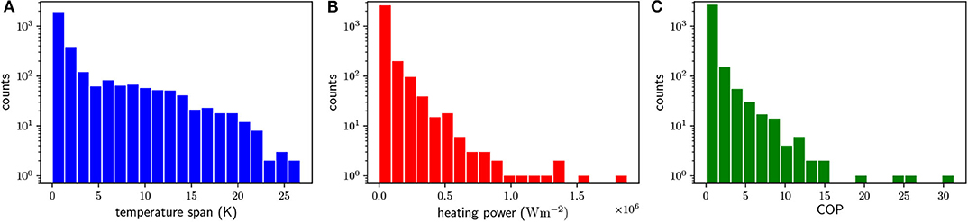
Figure 2. Histogram of the 3,000 computed systems, for the (A) temperature span, (B) cooling power, and (C) COP.
The goal of the present work is to dimension a magnetocaloric system without the need to perform intensive computation. For that end a method of predicting the output of computed systems is here exposed by using classifiers. The first step is to classify the 3,000 simulations into acceptable or not acceptable for the defined requirements. This new variable, goal G, will determine the class of each performed simulation. If it complies with the requirements G=1, if not G=0. After classifying the dataset one must balance the data, so that there are equal numbers of simulations with G=0 and G=1. To that end, the exceeding number of the most popular G value is removed randomly. At the end of the first treatment, each predictor must be normalized to 1, and is divided into a training dataset (60% of the data) and a testing dataset (40% of the data).
3. Classifiers
A classifier is an algorithm that maps input data to a specific class. Classifiers must be trained with training data for that purpose. In the present case, the trained classifiers must characterize a given system with G=0 or G=1. Seven different classifiers were considered in this work to find the most reliable method for dimensioning the system described above. Each one will be described and tested below for a requirement of a minimum temperature span of 4K. The whole analysis in this work was performed by using the Python sklearn module (skl, 2018).
3.1. K-Nearest Neighbors
The K-nearest neighbors (KNN) classifier is known as one of the most simple and straightforward classifier to implement (James et al., 2013). In the present case, the K nearest input parameters of the training dataset is used to determine the G variable. For that end, the average G for the K nearest neighbors is calculated by
where y is the vector that represents all the seven input parameters (predictors) of the machine that we want to predict the performance, and z represents the input parameters vector of one computed system of the training dataset. Taking Z as the set of all z vectors, ZK is a subset of Z that includes the K nearest z vectors to y. If Pr(x) > 0.5, than G=1, otherwise G=0. Depending on the K value, different prediction performances may arise, as depicted in Figure 3 for the error of the test dataset, i.e., fraction of bad predictions. For K values below ~ 13, the model results in under-fitting, i.e., larger values for K improves the precision of the model. For K values above ~ 13, the model results in over-fitting, i.e., larger values for K increases the complexity of the model beyond reality. Therefore K = 13 shows an error of less than 12%: 88% of the predictions are correct.
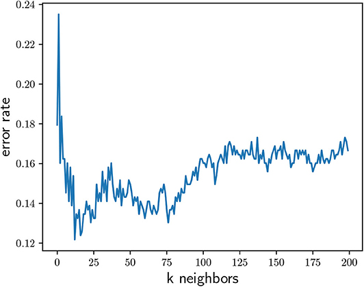
Figure 3. Error rate as a function of K neighbors for the KNN classifier.
3.2. Multilayer Perceptron
The Perceptron is one of the most famous classifiers (Bishop, 2006). It is well-known for its high accuracy, although its interpretation can be often complex. It consists of applying edge factors to the predictor nodes and inference of the class by using an activation function. By using hidden layers, instead of one for the predictor nodes as seen in Figure 4, the resulting classifier, known as multilayer Perceptron, is one of the most accurate. The value of each of the hidden nodes and output nodes is determined by
where Nm,j is the node value in layer m and index j, βm,j is a bias value, Nm−1 is the node set of layer m − 1, and αm,j,q are the coefficients for the determination of the node value Nm,j.
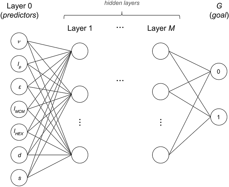
Figure 4. Used multilayer Perceptron model, with M hidden layers.
In this work a multilayer Perceptron was created for predicting the goal G. In that respect, a backpropagation algorithm was used and the best parameter for the perceptron was obtained by choosing the ones which showed the best performance according to a three-fold cross validation method (James et al., 2013). The parameter that were varied were the regularization term (α), which accounts for the a penalty to avoid the node coefficients αm,j,q to be very large, from 10−8 to 10−1, the learning rate (τ), which accounts for the weight of each training datum in the classifier, from 0.001 to 1, and the number (h) of nodes of the hidden layer. For this assessment only one hidden layer was used. The fitting procedure showed that if using h = 6, τ = 0.1, and α = 10−6 the resulting average f-score of 95% was largest. The f-score is the harmonic mean of the precision, which is the fraction of true positives over true positives plus false positives, and the recall, which is the fraction of true positives over the sum of true positives and false negatives. The resulting classifier shows a precision, recall and f-score for G=0 of 96, 94, and 95%, respectively, and 95, 96, and 95% for G=1, respectively.
3.3. Support Vector Machines
Support vector machines are classifiers that rely on hypersurfaces that divide different classes (Bishop, 2006; James et al., 2013). This division is dictated by the so-called kernel K. Different kernels represent different types of hypersurfaces, and depends on the predictor vector y and on the set of training data vectors Z. This way, each predictor point y is classified with the following function:
where η0 is a bias coefficient, and σi are prefactors. Each σi must be > 0 and < C, where C is the so-called tuning parameter (James et al., 2013). While η0 and σi values are determined during the training procedure, C must be pre-defined. In the present work four different kernels were considered, which will be described in the following. The respective precisions, recalls, and f-scores are in Table 2.

Table 2. Precision, recall, and f-score for G=0 and G=1 of the 4 support vector machine kernels.
3.3.1. Linear
The linear kernel for the support vector machine is simply the internal product of y and z:
Generally speaking, this classifier divides the two classes by a hyperplane. By using a three-fold cross validation, a fitting procedure was performed by varying C from 0.001 to 100. The fitting procedure showed that if using C = 100 the resulting average f-score of 92% was largest.
3.3.2. Polynomial
The polynomial kernel for the support vector machine is
where λ is a prefactor, r is a static coefficient and u is the polynomial degree. In this case the hypersurfaces are no longer linear, but follows a polynomial approach. By using a three-fold cross validation, a fitting procedure was performed by varying C from 0.001 to 1,000, by varying λ from 0.0001 to 1, by varying r from 0 to 1, for u=2 and u=3. The fitting procedure showed that if using C = 10, λ = 0.1, u=3, and r = 1 the resulting average f-score of 95% was largest.
3.3.3. RBF
The radial basis function (RBF) kernel for the support vector machine is
where ϕ is a prefactor. This classifier can use closed volumes for the classification. By using a three-fold cross validation, a fitting procedure was performed by varying C from 10−10 to 1010 and by varying ϕ from 10−15 to 105. The fitting procedure showed that if using C = 10, 000 and ϕ = 0.01, the resulting average f-score of 94% was largest.
3.3.4. Sigmoid
Finally, the sigmoid kernel for the support vector machine is
where tanh is the hyperbolic tangent, ψ is a prefactor and w is a static coefficient. By using a three-fold cross validation, a fitting procedure was performed by varying C from 0.01 to 10,000, by varying ψ from 0.0001 to 1, and by varying b from 0 to 1. The fitting procedure showed that if using C = 1, 000, ψ = 0.01, and b = 0 the resulting f-score of 91% was largest.
3.4. Random Forest
A decision tree classifier consists in stratifying, or segmenting, the predictor space into a number of simple regions (James et al., 2013). Although for some very simple problems decision trees are very easy to interpret, it does not have the same level of predictive accuracy when comparing to other classifiers. A Random forest classifier is a tree-based model that consists in building decision trees on bootstrapped training samples (James et al., 2013).
In the present work a fitting procedure with three-fold cross-validation was performed in order to obtain the best number of estimators, i.e., best number of predictor space segments. In that respect, it was considered a number of estimators ranging from 1 to 100. The best performance was obtained for 71 estimators. The resulting classifier showed a precision, recall and f-score for G=0 of 95, 91, and 93%, respectively, and 92, 96, and 94% for G=1, respectively. These numbers show that for the present case, random forests are comparable to other classifiers.
4. Statistical Modeling
So far, only the requirement of a minimum temperature span of 4K was considered. In this section, other requirements will be taken into account (temperature span, heating power, and COP), which will allow us to conclude which of the classifiers are more suited for each performance variable and for each range of values. In that respect, a continuous range of performance variables was investigated for all the classifiers described above, by using a fitting procedure that uses a three-fold cross validation. The details of the fitting parameters will be described below.
The variables for the fitting procedure of the KNN classifier were the number of K neighbors. For the linear kernel of the SVM it was varied the C value from 0.001 to 100. For the polynomial kernel, the C value ranged from 0.001 to 1,000, γ from 0.0001 to 1, and the considered polynomial degree was choosen between 2 and 3. For the RBF and sigmoid SVMs, the C value was varied from 10−10 to 1010 and from 0.01 to 10,000, respectively. While ϕ ranged from 10−15 to 105, ψ of the sigmoid kernel ranged from 0.0001 to 1, respectively. Moreover, the b value was varied from 0 to 1. Only the number of estimator was considered for the random forests fitting. Finally, for the multilayer Perceptron the α coefficient, the learning rate τ, and number of hidden nodes ranged from 10−8 to 10−1, from 0.001 to 1 and from 1 to 19, respectively.
4.1. Temperature Span
A range of temperature spans from 4K to 20K was considered in this work. Figure 5 shows the precision and recall for the two possible G values, as well as the average of the f-score. One can observe that the larger the temperature span the more fluctuations we have. This is due to the fact that the balanced dataset reduces with the temperature span, i.e., the larger the temperature span the less simulation from the dataset we have. Still, the accuracy of the predictions, i.e., the average f-score, is ≳ 90% for almost all classifiers and within the whole range of minimum temperature spans. Only the KNN classifier has an average f-score ≲ 90%. In fact, only for a temperature span of 16K and 20K other classifiers show smaller f-scores than the KNN one. From Figure 5 one can also note that, generally speaking, the precision and recall have similar values for all classifiers, so that the large f-scores does not result from only one of the precision or recall values. One interesting result is that the random forest classifier behaves in a similar manner as the support vector machine and multilayer Perceptron classifiers. Although they have very similar results, the multilayer Perceptron classifier is the one with the largest average (also over the temperature span) f-score.
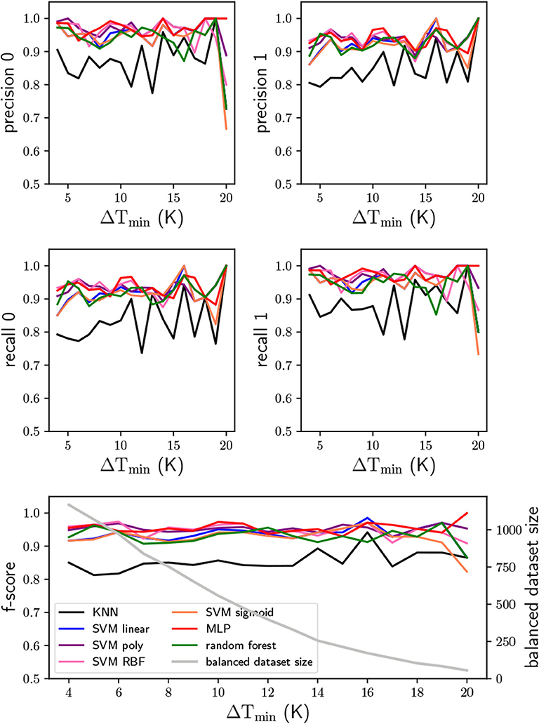
Figure 5. Precision and recall of the temperature span from 4K to 20K, for the two possibilities of the G variable (0 and 1), and the respective f-score average. In the f-score plot it is also shown the balanced dataset size.
4.2. Heating Power
The used values for the heating power ranged from 0.25 × 10⁶ to 0.95 × 10⁶ Wm−2. The precision and recall metrics can be seen in Figure 6. In this case the fluctuations already occur for the small heating power values, and increases with the heating power. These fluctuations have to do with the fact that the requirements are very strict for the considered range so that the balanced dataset size is very small. In fact, the balanced dataset has less than 250 simulations already for 0.25 × 10⁶ Wm−2, and reduces with the required heating power. By comparing with the temperature span requirement analysis, the balanced dataset decreases from 1,000 to 250 computed systems. Such low number of computed systems decreases the f-score, i.e., the predictor accuracy, from ≳ 90% to ≳ 80%. Moreover, with such small numbers one cannot conclude which classifier is more accurate in predicting the G variable. Either one needs to reduce the heating power requirement for the same dataset, or increase the number of computed systems in the dataset. This shows clearly the importance of having a robust number of balanced datasets after defining the requirements.
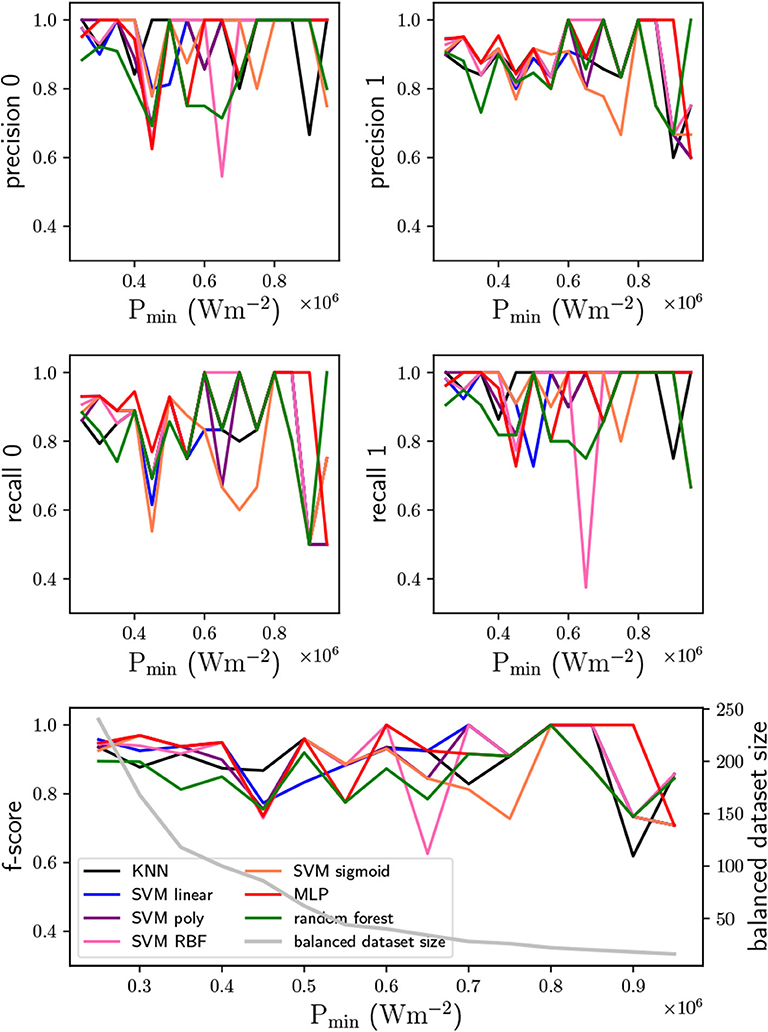
Figure 6. Precision and recall of the heating power from 0.25 × 10⁶ to 0.95 × 10⁶ Wm−2, for the two possibilities of the G variable (0 and 1), and the respective f-score average. In the f-score plot it is also shown the balanced dataset size.
4.3. COP
The used COP values ranged from 2 to 10. Similarly to the previous cases, the high intensity of the f-score fluctuations increases with the COP, as observed in Figure 7. Nevertheless, it is clear that the KNN is the worse classifier. This can be seen in Figure 7 in the f-score plot, where for COP=2 the KNN classifier has an f-score of ~ 85% while the other classifiers have an f-score above 93%. The balanced dataset size is between that of the heating power analysis and temperature span analysis, which explains why only above COP ~ 7, the f-score starts to show values below 90% for SVM, random forests and MLP classifiers.
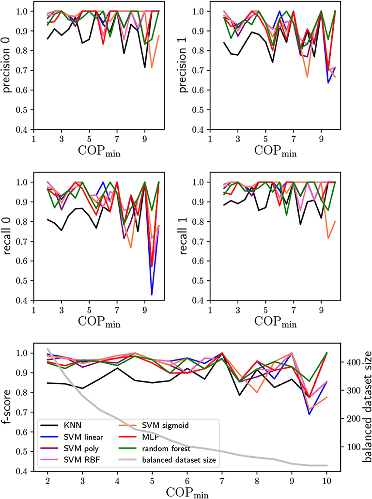
Figure 7. Precision and recall of the COP span from 2 to 10, for the two possibilities of the G variable (0 and 1), and the respective f-score average. In the f-score plot it is also shown the balanced dataset size.
5. System Dimensioning
In the previous section, the performance of different classifiers were analyzed for individual requirements, i.e., either a minimum temperature span, a minimum heating power or a minimum COP. In this section, one will impose a requirement involving all the three performance variables, through a three-fold filtering procedure, for a multilayer Perceptron and use the resulted classifier for dimensioning the 7 input parameters by computing simulations.
5.1. Three-Fold Filtering
To describe the overall process of dimensioning one will use an example with a requirement of 15K for the minimum temperature span, of 0.5 × 10⁶ Wm−2 for the minimum heating power, and a 3 for the minimum COP. By using the 3,000 computed systems used in the dataset of this work, and following the procedure described in the dataset subsection, i.e., procedure of balancing and normalizing the dataset, one arrives at 36 simulations with G=0 and 36 with G=1. With this resulting dataset, a multilayer Perceptron was trained with 60% of the data. The testing used 40% of the data, which resulted in an average f-score of 95%. This f-score shows the high performance of the classifier even though only 72 simulations were used.
5.2. Dimensioning by Computing Simulations
The method here proposed involves the computation of a large number of simulations with the trained classifier described in the previous subsection. We highlight the difference between the computation of simulations and the computation of systems used for obtaining the dataset. For the example shown above, the computation of simulations was performed for 8 values of ν ranging from 0.625 to 5 Hz, 7 of ϵ ranging from 0.357 to 2.5 mm, 7 lp ranging from 0.357 to 2.5 mm, 7 lMCM ranging from 1.423 to 10 cm, 7 lHEX ranging from 1.423 to 10 cm, 7 d ranging from 1.423 to 10 cm, and 7 s ranging from 1.423 to 10 cm, i.e., a total of 941,192 different combinations. The computation of simulations resulted in 894,287 combinations of input parameters with G=0, and 46,905 combinations with G=1. Since the final goal is to pick up 1 combination, a filtering procedure must be handled. For the present example, the filtering of the 46,905 combinations with ν < 1Hz, lMCM ≤ 8cm, 3cm ≤ s ≤ 5cm, d ≤ 2cm, lp ≥ 1mm, and d ≥ 1mm, resulted in 4 combinations. In all the possible combinations, the frequency ν was 0.625 Hz, s was 4.286 cm, lMCM was 7.143 cm, ϵ was 1.071 mm, lp was 1.071 mm, and d was 2.857cm. The only difference between the 4 possible combinations was the length of the heat exchangers that needs to be between 1.423 and 5.714 cm, i.e., the length of the heat exchangers does not influence considerably the performance of the system.
5.3. Summary of the Procedure
Figure 8 summarizes the method presented in this work for the dimensioning of magnetocaloric systems with statistical learning classifiers. First, a robust dataset must be computed. Then the requirements, defined by a parameter G (goal) must be applied to the dataset. Then, the dataset must be balanced and normalized. The resulting data is used to train and test a classifier (in the present case a multilayer Perceptron). If the resulting f-score is not acceptable one needs to increase the initial dataset and proceed with the workflow. If the f-score is acceptable, the classifier is used to mimic a very large number of simulations to produce a dataset of computed simulations, i.e., a huge number of mimicked simulations defined by a very large number of combinations of input parameters. Finally, since a significant number of combinations of parameters results in G=1, one needs to filter the input parameters of the dataset of computed simulations.
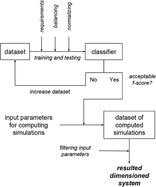
Figure 8. Scheme for the procedure to dimension magnetocaloric systems with statistical learning classifiers.
5.4. Computational Cost
The statistical learning method for dimensioning magnetocaloric systems proposed in this work can reduce by orders of magnitude the time consumed in computing numerically the performance of systems. In the example treated in this section it was mimicked the computation of 941,192 different systems by using a dataset of 3,000 simulations. It took approximately 4 years × core of computation for obtaining the 3,000 computed systems. If computing numerically the 941,192 different systems it would take approximately 1,250 years × core of computation, which is unfeasible. In the present study 25 different cores were used at the same time, so that the final computation time was 2 months. Since the computation of simulations lasted only a few hours, i.e., contributes marginally for the overall computation time, the time consumed with the present method is approximately of the time consumed if performing the computation of the 941,192 systems with a brute force approach.
6. Conclusions
We presented a method for the dimensioning of magnetocaloric systems by using statistical learning classifiers. The method consists in training a classifier and using it to mimic the numerical computation of a very large number of systems with different combinations of variables, e.g., frequency. With the resulting computed simulations, and by filtering some input variables, one is able to obtain a few combinations for the defined requirements.
We tested several statistical learning classifiers, and found out that, apart from the K-nearest neighbors classifier, support vector machines, multilayer Perceptrons and random forests present similar behaviors with high f-scores. We applied the method to one example where the heatrapy package was used to produce 3,000 computed systems, and showed that a multilayer Perceptron resulted in an f-score of 95% for a requirement of temperature span above 4K, heating power above 0.5 × 10⁶ Wm−2 and COP above 3. By mimicking 941,192 computed systems with the multilayer Perceptron classifier, and by filtering the 7 input parameters, we arrived at 4 different combinations of input variables. We emphasize that this method can be applied to any model (or software) for producing the dataset.
Data Availability Statement
The datasets generated for this study are available on request to the corresponding author.
Author Contributions
All authors provided substantial contributions to the conception or the work and interpretation of data. While DS drafted the work, JA and VA revised critically the manuscript. All authors provided approval for publication of the content.
Conflict of Interest
The authors declare that the research was conducted in the absence of any commercial or financial relationships that could be construed as a potential conflict of interest.
Acknowledgments
The present study was developed in the scope of the Smart Green Homes Project [POCI-01-0247-FEDER-007678], a co-promotion between Bosch Termotecnologia S.A. and the University of Aveiro. It is financed by Portugal 2020 under the Competitiveness and Internationalization Operational Program, and by the European Regional Development Fund. Project CICECO-Aveiro Institute of Materials, POCI-01-0145-FEDER-007679 (FCT Ref. UID/CT/5001/2013), financed by national funds through the FCT/MEC and co-financed by FEDER under the PT2020 Partnership Agreement is acknowledged. JA acknowledge FCT IF/01089/2015 grant.
References
Aprea, C., Greco, A., and Maiorino, A. (2013). A dimensionless numerical analysis for the optimization of an active magnetic regenerative refrigerant cycle. Int. J. Energ. Res. 37, 1475–1487. doi: 10.1002/er.2955
Aprea, C., Greco, A., Maiorino, A., and Masselli, C. (2017). A two-dimensional investigation about magnetocaloric regenerator design: parallel plates or packed bed? J. Phys. Conf. Ser. 796:012018. doi: 10.1088/1742-6596/796/1/012018
Aprea, C., and Maiorino, A. (2010). A flexible numerical model to study an active magnetic refrigerator for near room temperature applications. Appl. Energy 87, 2690–2698. doi: 10.1016/j.apenergy.2010.01.009
Bishop, C. M. (2006). Pattern recognition and machine learning. Springer, Springer-Verlag New York, 1st edition.
Bouchekara, H., Kedous-Lebouc, A., Yonnet, J., and Chillet, C. (2014). Multiobjective optimization of AMR systems. Int. J. Refrig. 37, 63–71. doi: 10.1016/j.ijrefrig.2013.09.009
Engelbrecht, K., Tušek, J., Nielsen, K., Kitanovski, A., Bahl, C., and Poredoš, A. (2013). Improved modelling of a parallel plate active magnetic regenerator. J. Phys. D 46:255002. doi: 10.1088/0022-3727/46/25/255002
Franco, V., Blázquez, J. S., Ingale, B., and Conde, A. (2012). The magnetocaloric effect and magnetic refrigeration near room temperature: materials and models. Annu. Rev. Mater. Res. 42:305. doi: 10.1146/annurev-matsci-062910-100356
Gschneidner, K. Jr., and Pecharsky, V. (2008). Thirty years of near room temperature magnetic cooling: where we are today and future prospects. Int. J. Refrig. 31:945. doi: 10.1016/j.ijrefrig.2008.01.004
hea. (2018). Source for the Heatrapy Package at Github, version v1.0.0. Available online at: https://github.com/djsilva99/heatrapy
James, G., Witten, D., Hastie, T., and Tibshirani, R. (2013). An Introduction to Statistical Learning, 1st Edn. New York, NY; Heidelberg; Dordrecht; London: Springer. doi: 10.1007/978-1-4614-7138-7
Kitanovski, A., Plaznik, U., Tomc, U., and Poredoš, A. (2015a). Present and future caloric refrigeration and heat-pump technologies. Int. J. Refrig. 57:288. doi: 10.1016/j.ijrefrig.2015.06.008
Kitanovski, A., Tušek, J., Tomc, U., Plaznik, U., Ožbolt, M., and Poredoš, A. (2015b). Magnetocaloric Energy Conversion: From Theory to Applications, 1st Edn. New York, NY; Heidelberg; Dordrecht; London: Springer. doi: 10.1007/978-3-319-08741-2
Lei, T., Engelbrecht, K., Nielsen, K., and Veje, C. (2017). Study of geometries of active magnetic regenerators for room temperature magnetocaloric refrigeration. Appl. Therm. Eng. 111, 1232–1243. doi: 10.1016/j.applthermaleng.2015.11.113
Li, J., Numazawa, T., Matsumoto, K., Yanagisawa, Y., and Nakagome, H. (2012). A modeling study on the geometry of active magnetic regenerator. AIP Conf. Proc. 1434, 327–334. doi: 10.1063/1.4706936
Li, P., Gong, M., and Wu, J. (2008). Geometric optimization of an active magnetic regenerative refrigerator via second-law analysis. J. Appl. Phys. 104:103536. doi: 10.1063/1.3032195
Ling, J., Jones, R., and Templeton, J. (2016). Machine learning strategies for systems with invariance properties. J. Comput. Phys. 318, 22–35. doi: 10.1016/j.jcp.2016.05.003
Lyubina, J. (2017). Magnetocaloric materials for energy efficient cooling. J. Phys. D Appl. Phys. 50:053002. doi: 10.1088/1361-6463/50/5/053002
mat. (2019). Matfinder Website. Available online at: https://matfinder.io
Matouš, K., Geers, M., Kouznetsova, V., and Gillman, A. (2017). A review of predictive nonlinear theories for multiscale modeling of heterogeneous materials. J. Comput. Phys. 330, 192–220. doi: 10.1016/j.jcp.2016.10.070
Moya, X., Kar-Narayan, S., and Mathur, N. D. (2014). Caloric materials near ferroic phase transitions. Nat. Mater. 13:439. doi: 10.1038/nmat3951
Nielsen, K., Bahl, C., Smith, A., Bjørk, R., Pryds, N., and Hattel, J. (2009). Detailed numerical modeling of a linear parallel-plate active magnetic regenerator. Int. J. Refrig. 32, 1478–1486. doi: 10.1016/j.ijrefrig.2009.03.003
Nielsen, K., Bahl, C., Smith, A., Pryds, N., and Hattel, J. (2010). A comprehensive parameter study of an active magnetic regenerator using a 2D numerical model. Int. J. Refrig. 33, 753–764. doi: 10.1016/j.ijrefrig.2009.12.024
Nielsen, K., Nellis, G., and Klein, S. (2013). Numerical modeling of the impact of regenerator housing on the determination of nusselt numbers. Int. J. Heat Mass Transf. 65, 552–560. doi: 10.1016/j.ijheatmasstransfer.2013.06.032
Nielsen, K., Tusek, J., Engelbrecht, K., Schopfer, S., Kitanovski, A., Bahl, C., et al. (2011). Review on numerical modeling of active magnetic regenerators for room temperature applications. Int. J. Refrig. 34, 603–616. doi: 10.1016/j.ijrefrig.2010.12.026
Niknia, I., Campbell, O., Christiaanse, T., Govindappa, P., Teyber, R., Trevizoli, P., et al. (2016). Impacts of configuration losses on active magnetic regenerator device performance. Appl. Therm. Eng. 106, 601–612. doi: 10.1016/j.applthermaleng.2016.06.039
Parish, E., and Duraisamy, K. (2016). A paradigm for data-driven predictive modeling using field inversion and machine learning. J. Comput. Phys. 305, 758–774. doi: 10.1016/j.jcp.2015.11.012
Petersen, T., Engelbrecht, K., Bahl, C., Elmegaard, B., Pryds, N., and Smith, A. (2008a). Comparison between a 1d and a 2d numerical model of an active magnetic regenerative refrigerator. J. Phys. D 41:105002. doi: 10.1088/0022-3727/41/10/105002
Petersen, T. F., Pryds, N., Smith, A., Hattel, J., Schmidt, H., and Høgaard Knudsen, H. J. (2008b). Two-dimensional mathematical model of a reciprocating room-temperature active magnetic regenerator. Int. J. Refrig. 31:432. doi: 10.1016/j.ijrefrig.2007.07.009
Risser, M., Vasile, C., Muller, C., and Noume, A. (2013). Improvement and application of a numerical model for optimizing the design of magnetic refrigerators. Int. J. Refrig. 36, 950–957. doi: 10.1016/j.ijrefrig.2012.10.012
Roudaut, J., Kedous-Lebouc, A., Yonnet, J.-P., and Muller, C. (2011). Numerical analysis of an active magnetic regenerator. Int. J. Refrig. 34, 1797–1804. doi: 10.1016/j.ijrefrig.2011.07.012
Roy, S., Poncet, S., and Sorin, M. (2017). Sensitivity analysis and multiobjective optimization of a parallel-plate active magnetic regenerator using a genetic algorithm. Int. J. Refrig. 75, 276–285. doi: 10.1016/j.ijrefrig.2017.01.005
Silva, D., Amaral, J., and Amaral, V. (2019a). Cooling by sweeping: a new operation method to achieve ferroic refrigeration without fluids or thermally switchable components. Int. J. Refrig. 101, 98–105. doi: 10.1016/j.ijrefrig.2019.02.029
Silva, D., Amaral, J., and Amaral, V. (2019b). Modeling and computing magnetocaloric systems using the python framework heatrapy. Int. J. Refrig. 106:278. doi: 10.1016/j.ijrefrig.2019.06.014
Silva, D. J., Amaral, J. S., and Amaral, V. S. (2018). Heatrapy: a flexible python framework for computing dynamic heat transfer processes involving caloric effects in 1.5D systems. SoftwareX 7, 373–382. doi: 10.1016/j.softx.2018.09.007
Silva, D. J., Bordalo, B. D., Pereira, A. M., Ventura, J., and Araújo, J. P. (2012). Solid state magnetic refrigerator. Appl. Energy 93:570. doi: 10.1016/j.apenergy.2011.12.002
Silva, D. J., Bordalo, B. D., Puga, J., Pereira, A. M., Ventura, J., Oliveira, J. C. R. E., et al. (2016). Optimization of the physical properties of magnetocaloric materials for solid state magnetic refrigeration. Appl. Therm. Eng. 99:514. doi: 10.1016/j.applthermaleng.2016.01.026
Silva, D. J., Ventura, J., Amaral, J. S., and Amaral, V. S. (2019c). Enhancing the temperature span of thermal switch-based solid state magnetic refrigerators with field sweeping. Int. J. Energ. Res. 43, 742–748. doi: 10.1002/er.4264
Silva, D. J., Ventura, J., Araújo, J. P., and Pereira, A. M. (2014). Maximizing the temperature span of a solid state active magnetic regenerative refrigerator. Appl. Energy 113:1149. doi: 10.1016/j.apenergy.2013.08.070
skl. (2018). Scikit-Learn Website. Available online at: http://scikit-learn.org/stable/
Tagliafico, G., Scarpa, F., and Tagliafico, L. (2012). Dynamic 1D model of an active magnetic regenerator: a parametric investigation. J. Mech. Eng. 58, 9–15. doi: 10.5545/sv-jme.2010.112
Tagliafico, G., Scarpa, F., and Tagliafico, L. (2013). A dimensionless description of active magnetic regenerators to compare their performance and to simplify their optimization. Int. J. Refrig. 36, 941–949. doi: 10.1016/j.ijrefrig.2012.10.024
Tishin, A. M., and Spichkin, Y. I. (2003). The Magnetocaloric Effect and its Applications, 1st Edn. Bristol: IOP Publishing. doi: 10.1887/0750309229
Trevizoli, P., Barbosa, J., Tura, A., Arnold, D., and Rowe, A. (2014). Modeling of thermomagnetic phenomena in active magnetocaloric regenerators. J. Therm. Sci. Eng. Appl. 6:031016. doi: 10.1115/1.4026814
Trevizoli, P., and Barbosa, J. R. Jr. (2017). Entropy generation minimization analysis of active magnetic regenerators. Anais da Academia Brasileira de Ciencias 89, 717–743. doi: 10.1590/0001-3765201720160427
Trevizoli, P., Nakashima, A., and Barbosa, J. R. Jr. (2016). Performance evaluation of an active magnetic regenerator for cooling applications-part II: mathematical modeling and thermal losses. Int. J. Refrig. 72, 206–217. doi: 10.1016/j.ijrefrig.2016.07.010
Trevizoli, P., Nakashima, A., Peixer, G., and Barbosa, J. R. Jr. (2017). Performance assessment of different porous matrix geometries for active magnetic regenerators. Appl. Energy 187, 847–861. doi: 10.1016/j.apenergy.2016.11.031
Tušek, J., Kitanovski, A., and Poredoš, A. (2013). Geometrical optimization of packed-bed and parallel-plate active magnetic regenerators. Int. J. Refrig. 36, 1456–1464. doi: 10.1016/j.ijrefrig.2013.04.001
Yu, B., Gao, Q., Zhang, B., Meng, X., and Chen, Z. (2003). Review on research of room temperature magnetic refrigeration. Int. J. Refrig. 26:622. doi: 10.1016/S0140-7007(03)00048-3
Yu, B., Liu, M., Egolf, P. W., and Kitanovski, A. (2010). A review of magnetic refrigerator and heat pump prototypes built before the year 2010. Int. J. Refrig. 33:1029. doi: 10.1016/j.ijrefrig.2010.04.002
Nomenclature
Greek
α Perceptron edge factor
β Perceptron bias coefficient
Δ Difference
ε Thickness of parallel plates (mm)
η SVM bias coefficient
λ Polynomial SVM prefactor
ν Frequency (Hz)
ϕ RBF SVM prefactor
ψ Sigmoid SVM prefactor
ρ Density (kgm−3)
σ SVM prefactor
Superscript
n Time index
Roman
C Specific heat at constant H (Jkg−1K−1)
CHEX Cold heat exchanger
COP Coeficient of performance
d Distance (mm)
G Goal variable
H Magnetic field (Am−1)
h Number of hidden layers
HEX Heat exchanger
HHEX Hot heat exchanger
K Number of nearest neigbors, or kernel
k Thermal conductivity (Wm−1K−1)
KNN K-nearest neigbors
l Axial length (mm)
M Number of hidden layers
MCM Magnetocaloric material
MLP Multilayer Perceptron
N Perceptron node
P Power (W)
Pr Probability function
Q Heat transfer power per volume (Wm−3)
r Polynomial SVM static coefficient
RBF Radial basis function
RF Random forest
s Stroke (mm)
SVM Support vector machine
T Temperature (K)
t Time (s)
u Polynomial degree
V Velocity (ms−1)
w Sigmoid SVM static coefficient
x Position (m)
y Predictors vector
Z Set of all training parameter vectors
z Training parameter vector
Subscript
ad Adiabatic
f Fluid
H At constant magnetic field
i Space index, or predictor index
j Perceptron node index
m Perceptron layer index
max Maximum
p Parallel plate
s Solid
Keywords: magnetocaloric, machine learning, statistical method, caloric materials, dimensioning algorithm
Citation: Silva DJ, Amaral JS and Amaral VS (2020) Broad Multi-Parameter Dimensioning of Magnetocaloric Systems Using Statistical Learning Classifiers. Front. Energy Res. 8:121. doi: 10.3389/fenrg.2020.00121
Received: 01 October 2019; Accepted: 19 May 2020;
Published: 23 June 2020.
Edited by:
Christian Bahl, Technical University of Denmark, DenmarkReviewed by:
Urban Tomc, University of Ljubljana, SloveniaWei Dai, Chinese Academy of Sciences (CAS), China
Copyright © 2020 Silva, Amaral and Amaral. This is an open-access article distributed under the terms of the Creative Commons Attribution License (CC BY). The use, distribution or reproduction in other forums is permitted, provided the original author(s) and the copyright owner(s) are credited and that the original publication in this journal is cited, in accordance with accepted academic practice. No use, distribution or reproduction is permitted which does not comply with these terms.
*Correspondence: Daniel J. Silva, ZGpzaWx2YUB1YS5wdA==