 Yangyi Zhang
 Xiafeng Zhou
- 1Department of Nuclear Engineering and Technology, School of Energy and Power Engineering, Huazhong University of Science and Technology, Wuhan, China
- 2Institute of Interdisciplinary Research for Mathematics and Applied Science, Huazhong University of Science and Technology, Wuhan, China
A parallel Jacobian-Free Newton Krylov discrete ordinates method (comePSn_JFNK) is proposed to solve the multi-dimensional multi-group pin-by-pin neutron transport models, which makes full use of the good efficiency and parallel performance of the JFNK framework and the high accuracy of the Sn method for the large-scale models. In this paper, the k-eigenvalue and the scalar fluxes (rather than the angular fluxes) are chosen as the global solution variables of the parallel JFNK method, and the corresponding residual functions are evaluated by the Koch–Baker–Alcouffe (KBA) algorithm with the spatial domain decomposition in the parallel Sn framework. Unlike the original Sn iterative strategy, only a “flattened” power iterative process which includes a single outer iteration without nested inner iterations is required for the JFNK strategy. Finally, the comePSn_JFNK code is developed in C++ language and, the numerical solutions of the 2-D/3-D KAIST-3A benchmark problems and the 2-D/3-D full-core MOX/UOX pin-by-pin models with different control rod distribution show that comePSn_JFNK method can obtain significant efficiency advantage compared with the original power iteration method (comePSn) for the parallel simulation of the large-scale complicated pin-by-pin models.
1 Introduction
The efficient parallel algorithms and the acceleration methods of discrete ordinates methods (Sn) (Carlson, 1953) for multi-dimensional large-scale neutron transport models are research hotspots in the reactor simulation field. In the past few decades, many parallel Sn neutron transport codes are developed by using overloading spatial domain decomposition (Bailey and Falgout, 2009) or Koch–Baker–Alcouffe (KBA) algorithms (Baker and Koch, 1998), including DENOVO (Evans et al., 2010), PARTISN (Alcouffe et al., 2005), NECP-hydra (Xu et al., 2018), ARES (Zhang et al., 2017) and so on. To accelerate the calculation of the original Sn iterative strategies based on the power iteration methods (PI), a batch of numerical methods can be employed, such as Wielandt shifts methods, Chebyshev acceleration methods, coarse mesh finite difference methods, diffusion synthetic acceleration method. In this paper, the parallel Jacobian-free Newton-Krylov (JFNK) (Knoll and Keyes, 2004) methods are adopted.
The JFNK methods have good computational efficiency due to the fast and robust convergence, which are widely used to solve the atmospheric convection problem (Hossain and Alam, 2012), the sea ice simulation (Yaremchu and Panteleev, 2022), two-phase flow calculation (Hajizadeh et al., 2018), the neutron diffusion/transport models (Gill, 2009; Knoll et al., 2011), thermal hydraulics simulation (Esmaili et al., 2020) and multi-physics coupled problems (Walker et al., 2019). Meanwhile, some popular multi-physics coupled environments (or platforms), such as MOOSE (Gaston et al., 2009), LIME (Pawlowski et al., 2011) and VERA (Turner et al., 2016), employ the JFNK framework to solve the complicated reactor coupled systems. Recently, we have also developed an efficient JFNK framework based on coarse mesh finite difference and nodal expansion method in the COupling Multiphysics Environment (COME) to solve the steady/transient neutronics and neutronics-thermal hydraulic coupled problems (Zhou, 2022a; Zhou, 2022b; Zhou et al., 2022; Zhou, 2023). To take advantages of the good efficiency and parallel performance of the JFNK framework in COME, in this paper, the parallel JFNK method is combined with the parallel Sn method to solve the multi-dimensional large-scale neutron transport models.
Therefore, a parallel Jacobian-free Newton Krylov discrete ordinates method (comePSn_JFNK) is proposed to solve the multi-dimensional multi-group pin-by-pin neutron transport k-eigenvalue problems, which makes full use of the fast and robust convergence of the parallel JFNK framework and the high accuracy of the Sn method based on the KBA algorithm. The key to implement the JFNK framework into the Sn algorithm is to choose the k-eigenvalue and the scalar fluxes (rather than the angular fluxes) as the global solution variables for parallel JFNK, which are the minimal subset of the non-linear system. The corresponding residual functions are directly constructed from the neutron transport equations and evaluated based on the parallel Sn transport sweeping process by using a “flattened” power iterative process including a single outer iterative step without nested inner iterations.
This paper is organized as follows. The detailed theories of the comePSn_JFNK method are presented in Section 2, including the parallel JFNK method, the parallel Sn method, the residual function evaluation and the solution strategies. In Section 3, the numerical results for the 2-D/3-D full-core pin-by-pin models are analyzed to test the accuracy and efficiency of the comePSn_JFNK method. The conclusions are given in Section 4.
2 Methodologies of the comePSn_JFNK method
2.1 Parallel JFNK
JFNK method is one of the inexact Newton-Krylov methods, which are the combinations of Newton’s methods for solving non-linear equations, Krylov subspace methods for solving the linear Newton correction equations, and “Jacobian-free” technology for approximately solving Jacobian-vector product (Knoll and Keyes, 2004). The non-linear equations can be generally written by
where
where
For the parallel JFNK method, only the residual functions, the dot products and the norms of vectors are considered to be evaluated synchronously in multiple processors, which are easily developed in the parallel framework. In addition, residual functions are evaluated from the parallel Sn method based on KBA sweeping algorithm as shown in the following sections.
2.2 Evaluation of residual functions from parallel Sn
The multi-group neutron Boltzmann transport equations for the k-eigenvalue problem can be written as
where
Eq. 3 can be written in operator notation form as
where
Multiplied by
It is an eigenvalue problem, whose solution is to get an eigenpair vector
where
For each outer iteration, Eq. 7 is equivalent to a fixed source problem, which can generally be calculated using fixed point iteration method (which is the inner iteration) as
where
Meanwhile,
Then, according to the PI strategy for the parallel Sn method as shown in Eq. 7 and Eq. 8, the corresponding residual functions for the parallel JFNK method can be easily expressed as
where
where the evaluation is equivalent to a “flattened” power iterative process (Gill, 2009) including a single outer iteration without nested inner iterations as shown in Eq. 10. In this paper, the combined strategy of the parallel JFNK method and the parallel Sn method is called comePSn_JFNK method.
2.3 Parallel code design for evaluation of residual functions
In this paper, the comePSn and comePSn_JFNK codes are parallelly designed on spatial domain decomposition with the Message Passing Interface (MPI) standard. For the comePSn_JFNK code, the message communication between MPI ranks is mainly required for the evaluation of the residual functions, the dot products and the norms. The parallel dot products and norms of vectors can be easily calculated by using the MPI_Allreduce function. And the evaluation of residual functions employs the KBA algorithm, which can directly calculate the inversion of
KBA is constructed on the (N-1)-dimensional spatial domain decomposition for N-dimensional models. For 3-D rectangular coordinate system, the spatial grid is divided into domains on the XY layout of CPU cores (or MPI ranks). Each domain is further decomposed into computational chunks, which are solved in the “wavefront” ordering. Each computational chunk, in a single octant with N/8 discrete angles for a single energy group, is solved after receiving the incoming angular fluxes from the upstream chunks (or from the boundary conditions), and then the outer angular fluxes are sent to the downstream chunks if required. The “simultaneous in angle, successive in quadrants” pipelining method described in the reference (Baker and Koch, 1998) are chosen in this paper. In addition, to reduce the idle time, the sweeps start at all the four corners of the spatial grid at the same time (Bailey and Falgout, 2009).
As mentioned above, the KBA transport sweeping process can be easily applied to evaluate the residual functions for the parallel JFNK framework. In this work, the evaluation of the residual functions is a three-step process. 1) Map
2.4 Solution strategy
Based on the above methodologies, the parallel comePSn_JFNK and comePSn codes are respectively developed in the unified COME using C++ language to study the numerical accuracy, the efficiency and the parallel performance for the 3-D/2-D pin-by-pin neutron transport models. The iterative strategies and the flowchart are shown in Figure 1. The good initial guess
where
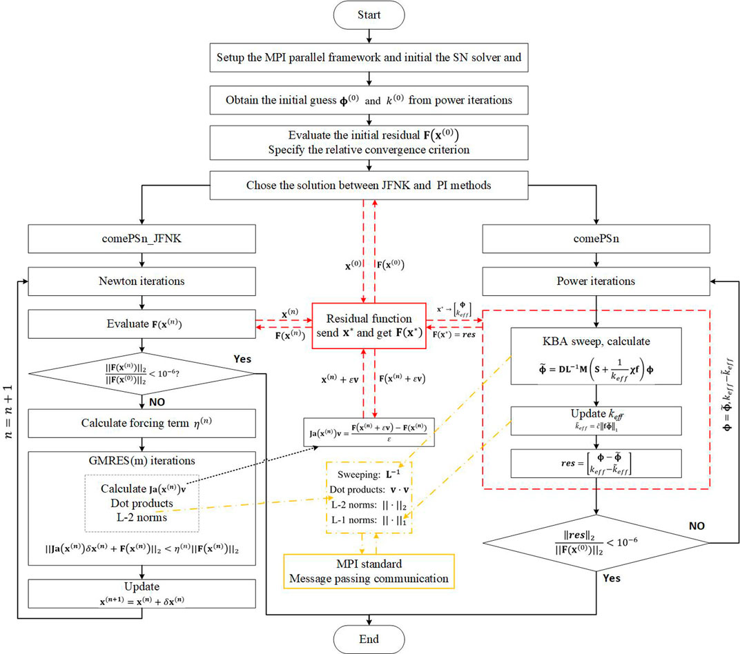
FIGURE 1. Iterative strategies and flowchart for the comePSn_JFNK and comePSn methods.
The restarted GMRES (Generalized Minimal REsidual) method (Saad and Schultz, 1986) is adopted to solve Eq. 15 and the maximum Krylov subspace dimension is set to 20. At last, the global convergent backtracking algorithm (Eisenstat and Walker, 1994) is employed to ensure the global convergence of come_PSn_JFNK.
3 Numerical results and analysis
In this section, we apply the comePSn_JFNK and comePSn codes to two series of complicated multi-dimensional pin-by-pin neutron transport models. First, the popular 2-D/3-D KAIST-3A benchmark problems with Gd burnable absorbers are simulated to analyze the numerical accuracy, the parallel performance and the computational efficiency of the comePSn_JFNK and comePSn codes. Then, the more complicated 2-D/3-D full-core MOX/UOX pin-by-pin models with different insertion forms of the control rods are further employed to test the high numerical efficiency of the comePSn_JFNK code compared with the comePSn code in an order of 1000 CPU cores on the computer clusters with Hygon C86 7185 32-core processors. In all of our numerical simulations, the S8 Carlson quadrature set (Longoni, 2004) is adopted to discretize the angular direction space.
3.1 KAIST-3A benchmark problem
KAIST-3A benchmark problems are published by KAIST Nuclear Reactor Analysis and Particle Transport laboratory (Cho, 2000), whose model is a simplified PWR core. The quarter symmetric radial geometry is illustrated in Figure 2. The core consists of two types of fuel assemblies, Uranium (UOX, including UOX-1 with 2.0% enrichment and UOX-2 with 3.3% enrichment) and Plutonium (MOX), which are surrounded by the baffle and reflector. Each fuel assembly follows a 17 × 17 lattice design of 21.42 cm width with a 1.26 cm pin pitch, which includes 264 fuel rods (or burnable absorber rods), 24 guide tubes (or control rods inserted) and one instrument guide tube as shown in Figure 3. There are two cases: all rods out (ARO) and all rods in (ARI), based on the configurations with or without the control rods (CR) inserted into the four UOX-2 fuel assemblies. Seven-group macroscopic cross sections are provided in the benchmark report, including UO2 fuel, MOX fuel, guide tube, BA (Burnable absorber) rod, control rod, baffle and reflector.
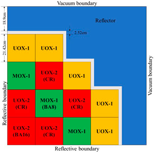
FIGURE 2. Radial geometry of the KAIST-3A benchmark problem.
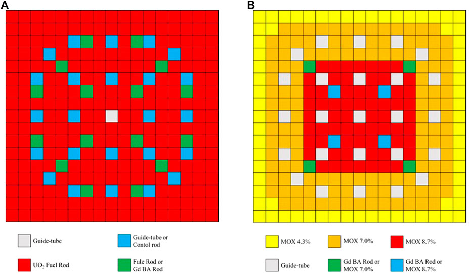
FIGURE 3. Fuel assembly configuration of the KAIST-3A benchmark problem: (A) UOX fuel assembly and (B) MOX fuel assembly.
At first, the 2-D quarter symmetric models are simulated by comePSn_JFNK and comePSn codes. The pin cell is divided into 1 × 1, 2 × 2, 4 × 4 and 32 × 32 rectangular meshes, respectively.
Table 1 and Figure 4 respectively show the comparison of the k-eigenvalue and the relative errors (%) of power density for ARO and ARI with different mesh sizes per pin using comePSn_JFNK and comePSn codes. It can be seen that there is no obvious difference between the results from the two codes. To further analyze the accuracy of the two codes with different mesh sizes per pin, the relative errors (%) of pin-wise power density on 1 × 1, 2 × 2 and 4 × 4 meshes per pin are presented in Figure 5 compared with the results on 32 × 32 meshes per pin. For 1 × 1 mesh per pin, the maximum value of the relative errors reaches 12% for ARO and 18% for ARI, and the errors of the k-eigenvalues are about 200 pcm (for ARO) and 750 pcm (for ARI). While for 2 × 2 and 4 × 4 meshes per pin, the errors of the power density and the k-eigenvalues are respectively less than 2% and 50 pcm, and it indicates that the solution on 2 × 2 meshes per pin can obtain acceptable numerical accuracy.
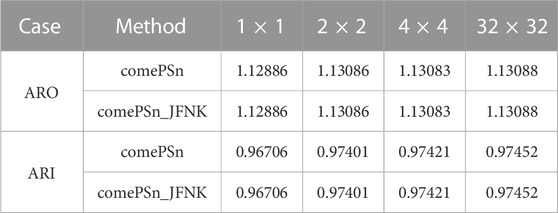
TABLE 1. Results of k-eigenvalues on different mesh sizes per pin for 2-D KAIST-3A benchmark problems.
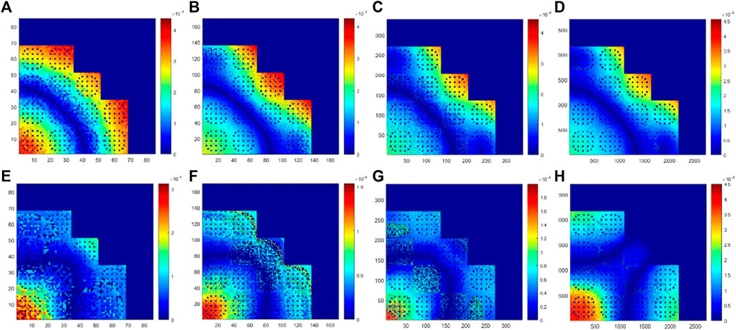
FIGURE 4. Relative error (%) of power density between comePSn_JFNK and comePSn codes on different mesh sizes per pin for 2-D KAIST-3A benchmark problems: (A) 1 × 1 for ARO, (B) 2 × 2 for ARO, (C) 4 × 4 for ARO, (D) 32 × 32 for ARO, (E) 1 × 1 for ARI, (F) 2 × 2 for ARI, (G) 4 × 4 for ARI and (H) 32 × 32 for ARI.
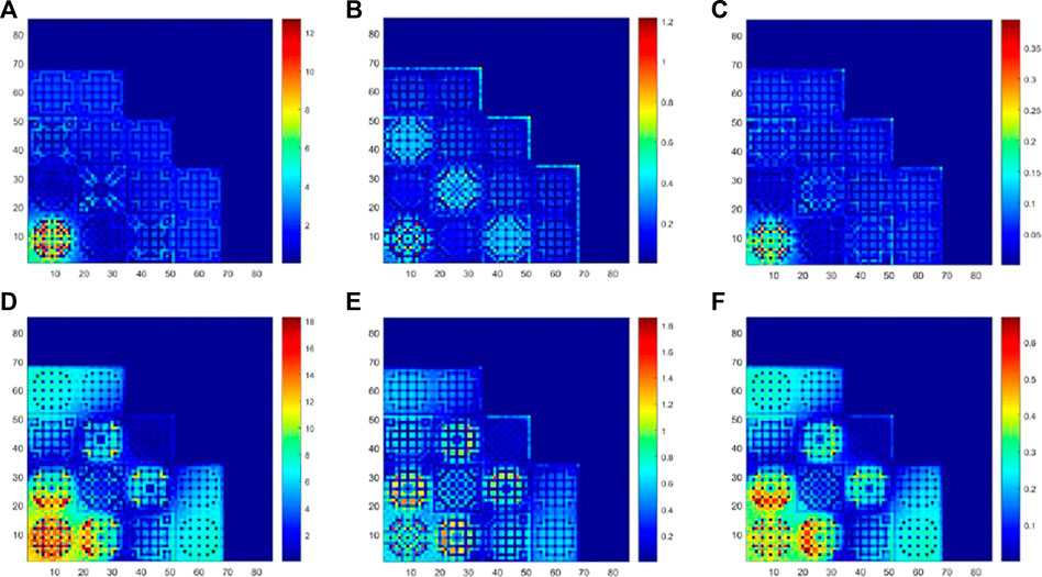
FIGURE 5. Relative error (%) of pin-wise power density on different mesh sizes per pin compared with those on 32 × 32 meshes per pin for 2-D KAIST-3A benchmark problems using the comePSn_JFNK code: (A) 1 × 1 for ARO, (B) 2 × 2 for ARO, (C) 4 × 4 for ARO, (D) 1 × 1 for ARI, (E) 2 × 2 for ARI and (F) 4 × 4 for ARI.
To further analyze the numerical efficiency of comePSn_JFNK and comePSn codes, the CPU times and iteration numbers are presented in Table 2. It should be noted that the CPU times do not include the cost of the initialization, reading the input files and writing the output files. The results indicate that the different mesh sizes per pin make no obvious difference on the convergence rate for both comePSn_JFNK and comePSn codes. The computational efficiency of the comePSn_JFNK code is about 6–8 times as much as the comePSn code for ARO and about 8–10 for ARI.
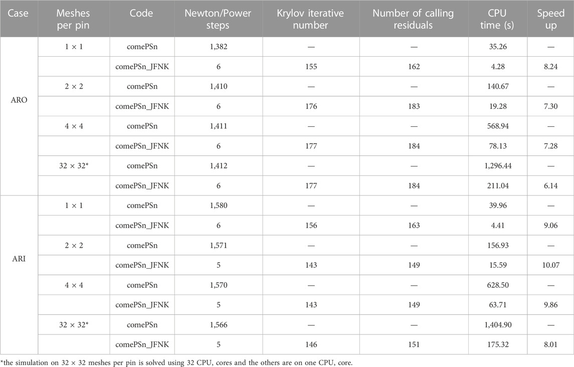
TABLE 2. Comparison of the computational cost for 2-D KAIST-3A benchmark problems.
Then the KAIST-3A 2-D quarter symmetric models are extend to 3-D full-core models with the same radial configuration, and axial reflectors are set at the top/bottom of the core. The active fuel length is 365.76 cm and the width of axial reactors is 21.42 cm. The control rods can be inserted from the top of the upper reflector to the bottom of the active fuel region in the UOX-2 (CR) assemblies. ARO and ARI cases are still simulated by comePSn_JFNK and comePSn codes.
The 3-D full-core model is divided into 340 × 340 × 340 meshes. Specifically, one pin cell is divided into 2 × 2 meshes in the radial direction; in the axial direction, the active region is divided into 300 meshes and the top/bottom reflectors are respectively divided into 20 meshes. Both comePSn_JFNK and comePSn codes solve the problems using 100 CPU cores. Figure 6 presents the relative errors (%) of radial average power density between the two codes and Figure 7 shows the radial average power density and 3-D power density distribution in the active regions calculated the comePSn_JFNK code. The numerical results of radial power density and the k-eigenvalues from the two codes also agree well with each other. The k-eigenvalues are respectively 1.12612 for ARO and 0.97063 for ARI.
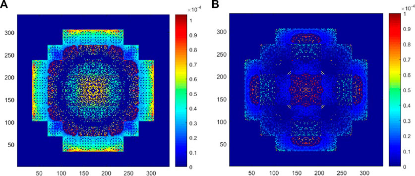
FIGURE 6. Relative error (%) of radial average power density between comePSn_JFNK and comePSn codes for 3-D KAIST-3A benchmark problems: (A) ARO and (B) ARI.

FIGURE 7. Radial average power density and 3-D power density distribution for 3-D KAIST-3A benchmark problems using the comePSn_JFNK code: (A) radial power density for ARO, (B) 3-D power density for ARO, (C) radial power density for ARI and (D) 3-D power density for ARI.
To further analyze the efficiency of comePSn_JFNK and comePSn codes for 3-D models, the iterative properties and CPU times (on 100 CPU cores) are listed in Table 3. Compared with the comePSn code, the speedups of the comePSn_JFNK code are 12.41 for ARO and 14.64 for ARI. It is worth noting that the acceleration rates of the comePSn_JFNK code for 3-D models are higher than those for 2-D models, which shows the advantage of numerical efficiency of the comePSn_JFNK code for the complicated 3-D neutron transport problems.
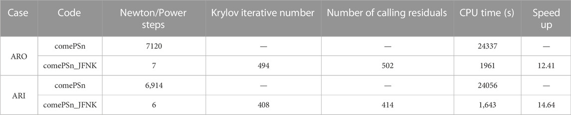
TABLE 3. Comparison of the computational cost for 3-D KAIST-3A benchmark problems (100 CPU cores).
In addition, the parallel efficiencies of the comePSn_JFNK code for the 3-D KAIST-3A ARO case using 4, 16, 100 and 400 CPU cores are shown in Figure 8. The “Solving” curve means the parallel efficiency of the total CPU time and the “Sweeping” curve indicates the parallel efficiency of KBA sweeping. The efficiencies of “Solving” and “Sweeping” using 400 CPU cores are respectively about 63% and 68%, which can be further improved by optimizing the parallel performance of the Krylov subspace methods and the strategies of the KBA algorithm.
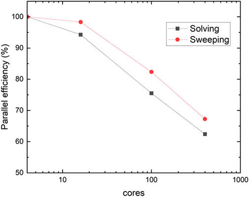
FIGURE 8. Parallel efficiency for 3-D KAIST-3A ARO case of the comePSn_JFNK code.
3.2 Full-core MOX/UOX pin-by-pin models
A series of 3-D/2-D PWR full-core MOX/UOX pin-by-pin models with different insertion positions of control rods are simulated to further study the numerical properties of comePSn_JFNK and comePSn codes. The reactor core also consists of UOX and MOX fuel assemblies surrounded by reflector. As shown in Figure 9, each fuel assembly is 21.42 cm wide and is made up of 17 × 17 lattice with a 1.26 cm pin pitch, which includes 264 fuel pins, 24 guide tubes (or control rods inserted) and one instrument tube for fission chamber. The UOX and MOX assemblies are distributed in a checker-board configuration and four core models (A, B, C and D) are designed with different configurations of the UOX assemblies with control rods inserted (UOA) as illustrated in Figure 10. The active fuel length is 365.76 cm and there are 21.42 cm high axial reflectors at the top/bottom of the core just as the 3-D KAIST-3A models. It should be noted that the control rods are inserted form the top of the upper reflector to the bottom of the active fuel regions in the models B, C and D; and the control rods are still in the upper reflector if withdrawn in the models A, C and D. In this paper both 2-D and 3-D models are simulated by comePSn_JFNK and comePSn codes. The seven-group cross sections for pin cells are chosen form the C5G7 benchmark report (Smith et al., 2005). The pin cells are divided into 2 × 2 rectangular meshes in the radial direction; in the axial direction, the active fuel region is divided into 580 meshes and the top/bottom reflectors are respectively divided into 30 meshes.
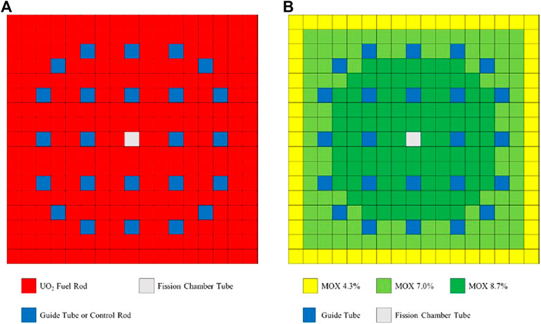
FIGURE 9. Fuel assembly configuration of the full-core MOX/UOX pin-by-pin models: (A) UOX fuel assembly and (B) MOX fuel assembly.
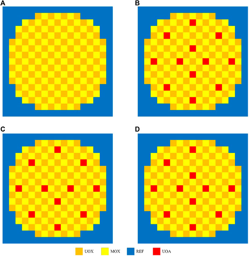
FIGURE 10. Radial core configuration of the full-core MOX/UOX pin-by-pin models: (A) model A, (B) model B, (C) model C and (D) model D.
Table 4 shows the results of the k-eigenvalues from comePSn_JFNK and comePSn codes and the reference solution is from the paper (Zhou, 2022a). It can be observed that the errors of k-eigenvalues from the two codes are about 150 pcm compared with the reference. Figure 11 shows the power density distribution from the comePSn_JFNK code and Figure 12 shows the corresponding relative errors (%) compared with the comePSn code. It can be observed that the power density distribution from the two codes agree well with each other, and even in the model B where the control rods are all inserted in, the maximum of the errors is less than 0.002%.
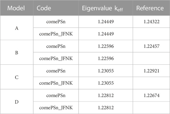
TABLE 4. Results of k-eigenvalues for 2-D full-core MOX/UOX pin-by-pin models A–D.
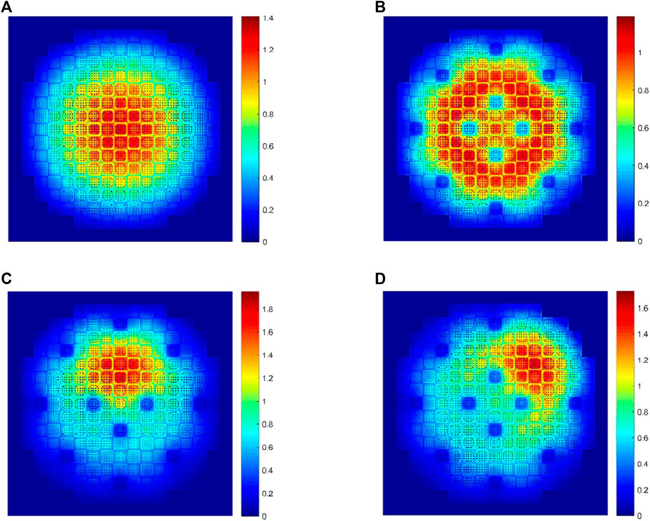
FIGURE 11. Power density distribution using the comePSn_JFNK code for 2-D full-core MOX/UOX pin-by-pin models: (A) model A, (B) model B, (C) model C and (D) model D.
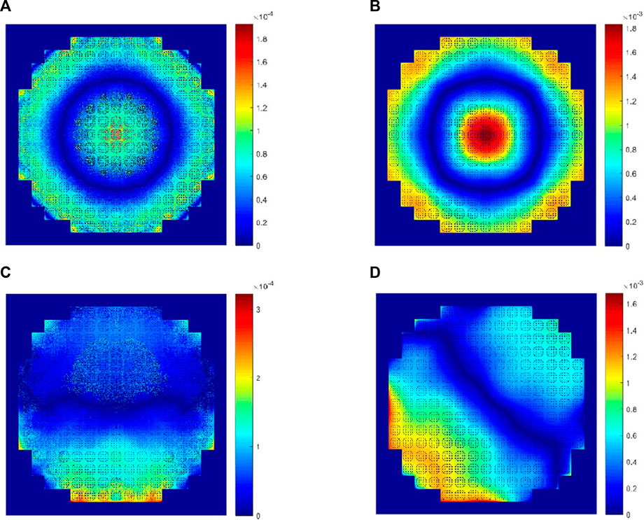
FIGURE 12. Relative errors (%) of radial average power density between comePSn_JFNK and comePSn codes for 2-D full-core MOX/UOX pin-by-pin models: (A) model A, (B) model B, (C) model C and (D) model D.
To analyze the numerical efficiency, Table 5 presents the comparation of the computational cost for the 2-D models from comePSn_JFNK and comePSn codes (using 1 core). Compared with the comePSn code, the speedups of the comePSn_JFNK code are respectively 15.40, 16.84, 29.90, and 29.67 for models A–D, which indicates that the acceleration rate of the comePSn_JFNK code for the asymmetric models C and D is higher than that for the symmetric models A and B. In addition, there is obvious difference of the iterative steps between the four models from the comePSn code, which range from 7093 to 27041. While the comePSn_JFNK code takes similar non-linear iterative steps (range from 5 to 10) due to the robust convergence of the JFNK methods.
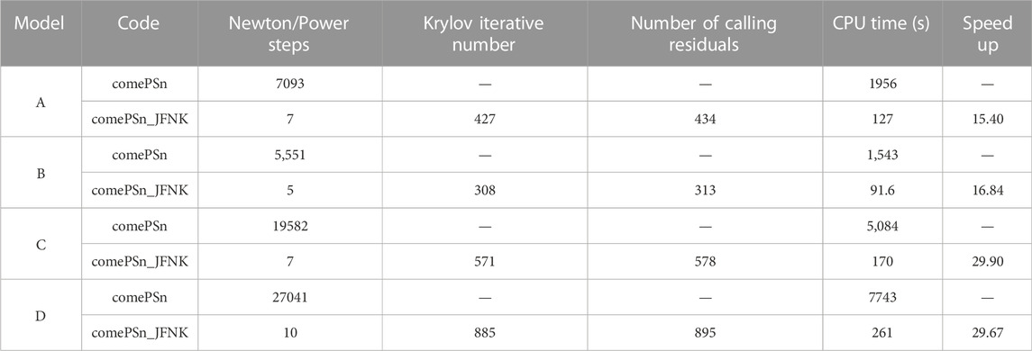
TABLE 5. Comparison of the computational cost for 2-D Full-core MOX/UOX pin-by-pin models A–D.
To further test the computational properties of the comePSn_JFNK code for 3-D models, the radial average power density and the 3-D power density distribution calculated by the comePSn_JFNK code using 1024 CPU cores are presented in Figure 13, and the k-eigenvalues and the computational cost compared with the comePSn code is shown in Table 6. It can be seen that the acceleration rate of the comePSn_JFNK code are respectively 20.48, 22.57, 24.93 and 26.45 for models A– D, which indicates that the comePSn_JFNK code still has significant efficiency advantage for the complicated 3-D full-core pin-by-pin models with different control rod distributions.
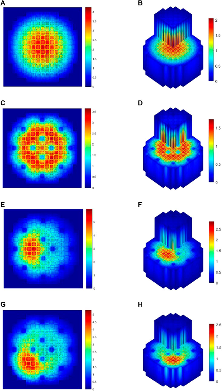
FIGURE 13. Radial average power and 3-D power density distribution for 3-D Full-core MOX/UOX pin-by-pin models: (A) radial power density for model A, (B) 3-D power density for model A, (C) radial power density for model B, (D) 3-D power density for model B, (E) radial power density for model C, (F) 3-D power density for model C, (G) radial power density for model D and (H) 3-D power density for model D.
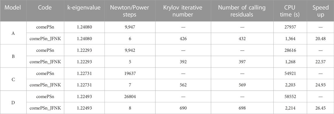
TABLE 6. Comparison of the k-eigenvalues and the computational cost for 3-D full-core MOX/UOX pin-by-pin models (1024 CPU cores).
4 Conclusion
In this paper, a parallel Jacobian-free Newton Krylov discrete ordinates method (comePSn_JFNK) is developed to solve the multi-dimensional multi-group pin-by-pin neutron transport problems, which combines the parallel JFNK framework and the parallel Sn method based on KBA algorithm. The comePSn_JFNK code exhibits the good efficiency compared with the traditional parallel Sn code with power iterative strategy (comePSn). Furthermore, by making full use of transport sweeping iterative framework, the corresponding residual functions of the parallel JFNK framework can be easily evaluated by only a “flattened” power iterative process which includes a single outer iteration without nested inner iterations. The comePSn_JFNK and the comePSn codes are developed in the unified COupled Multiphysics Environment (COME).
By simulating the 2-D/3-D KAIST-3A pin-by-pin benchmark problems and the 2-D/3-D full-core pin-by-pin MOX/UOX models, the speedups of the comePSn_JFNK code are 6–15 for the KAIST-3A benchmark problems and 15–30 for the full-core MOX/UOX pin-by-pin models, which indicates the comePSn_JFNK code has significant efficiency advantage for complicated 3-D full-core pin-by-pin models. Further study is to improve the parallel efficiency on the massively parallel computers, to apply the parallel coarse mesh finite difference methods and the parallel diffusion synthetic acceleration method as preconditioners, and to extend the comePSn_JFNK method to solve the pin-by-pin multi-physics coupled problems.
Data availability statement
The original contributions presented in the study are included in the article/Supplementary Material, further inquiries can be directed to the corresponding author.
Author contributions
YZ: Software, modeling, validation, data analysis and original draft preparation. XZ: Conception, methodology, software, review, editing and supervision.
Funding
This research was funded by National Natural Science Foundation of China: 12005073; National Key Research and Development Program of China: 2018YFE0180900; National Key Research and Development Program of China: 2020YFB1901600; Project of Nuclear Power Technology Innovation Center of Science Technology and Industry for National Defense: HDLCXZX-2021-HD-033.
Conflict of interest
The authors declare that the research was conducted in the absence of any commercial or financial relationships that could be construed as a potential conflict of interest.
Publisher’s note
All claims expressed in this article are solely those of the authors and do not necessarily represent those of their affiliated organizations, or those of the publisher, the editors and the reviewers. Any product that may be evaluated in this article, or claim that may be made by its manufacturer, is not guaranteed or endorsed by the publisher.
References
Alcouffe, R. E., Baker, R. S., Dahl, J. A., Davis, E. J., Saller, T. G., and Turner, S. A. (2005). Partisn: A time-dependent parallel neutral Particle transport code system. LAUR-05-3925 (Los Alamos, NM, USA: Los Alamos National Laboratory).
Bailey, T. S., and Falgout, R. D. “Analysis of massively parallel discrete-ordinates transport sweep algorithms with collisions,” in Proceedings of the International Conference on Mathematics, Computational Methods & Reactor Physics, Saratoga Springs, NY, USA, May 2009.
Baker, R. S. (2017). An SN algorithm for modern architectures. Nucl. Sci. Eng. 185, 107–116. doi:10.13182/nse15-124
Baker, R. S., and Koch, K. R. (1998). An Sn algorithm for the massively parallel CM-200 computer. Nucl. Sci. Eng. 128, 312–320. doi:10.13182/nse98-1
Carlson, B. G. (1953). Solution of the transport equation by Sn approximations. LA-1599 (Los Alamos, NM, USA: Los Alamos Scientific Laboratory Report).
Cho, N. Z. (2000). Daejeon, South Korea: Korea Advanced Institute of Science and Technology benchmark report. Available at: https://github.com/nzcho/Nurapt-Archives/tree/master/KAIST-Benchmark-Problems. Benchmark problem 3A: MOX fuel-loaded small PWR coreMOX Fuel Zoning, 7 Group Homog. Cells.
Eisenstat, S. C., and Walker, H. F. (1996). Choosing the forcing terms in an inexact Newton method. SIAM J. Sci. Comput. 17, 16–32. doi:10.1137/0917003
Eisenstat, S. C., and Walker, H. F. (1994). Globally convergent inexact Newton methods. SIAM J. Optim. 4, 393–422. doi:10.1137/0804022
Esmaili, H., Kazeminejad, H., Khalafi, H., and Mirvakili, S. (2020). Subchannel analysis of annular fuel assembly using the preconditioned Jacobian-free Newton Krylov methods. Ann. Nucl. Energy 146, 107616. doi:10.1016/j.anucene.2020.107616
Evans, T. M., Stafford, A. S., Slaybaugh, R. N., and Clarno, K. T. (2010). Denovo: A new three-dimensional parallel discrete ordinates code in scale. Nucl. Technol. 171, 171–200. doi:10.13182/nt171-171
Gaston, D., Newman, C., Hansen, G., and Lebrun-Grandie, D. (2009). Moose: A parallel computational framework for coupled systems of nonlinear equations. Nucl. Eng. Des. 239, 1768–1778. doi:10.1016/j.nucengdes.2009.05.021
Gill, D. F. (2009). “Newton-Krylov methods for the solution of the k-eigenvalue problem in multigroup neutronics calculations,”. PhD thesis (Pennsylvania, PA, USA: Pennsylvania State University).
Hajizadeh, A., Kazeminejad, H., and Talebi, S. (2018). Formulation of a fully implicit numerical scheme for simulation of two-phase flow in a vertical channel using the Drift-Flux Model. Prog. Nucl. Energy 103, 91–105. doi:10.1016/j.pnucene.2017.11.009
Hossain, M. A., and Alam, J. M. (2012). Assessment of a symmetry-preserving JFNK method for atmospheric convection. Comput. Phys. Commun. 269, 108113. doi:10.1016/j.cpc.2021.108113
Knoll, D. A., and Keyes, D. E. (2004). Jacobian-free Newton–Krylov methods: A survey of approaches and applications. J. Comput. Phys. 193, 357–397. doi:10.1016/j.jcp.2003.08.010
Knoll, D. A., Park, H., and Newman, C. (2011). Acceleration of k-eigenvalue/criticality calculations using the jacobian-free Newton-Krylov method. Nucl. Sci. Eng. 167 (2), 133–140. doi:10.13182/nse09-89
Longoni, G. (2004). Advanced quadrature sets and acceleration and preconditioning techniques for the discrete ordinates method in parallel computing environments. PhD Thesis (Gainesville, FL, USA: University of Florida).
Pawlowski, R., Bartlett, R., Belcourt, N., Cannon, S. R., and Warren, H. R. (2011). A theory manual for multi-physics code coupling in LIME, version 1.0. SAND2011-2195 (Albuquerque, NM, USA: SAND Report).
Saad, Y., and Schultz, M. H. (1986). Gmres: A generalized minimal residual algorithm for solving nonsymmetric linear systems. SIAM J. Sci. Stat. Comput. 7, 856–869. doi:10.1137/0907058
Smith, M. A., Lewis, E. E., and Na, B. C. (2005). Benchmark on deterministic transport calculations without spatial homogenization: MOX fuel assembly 3-D extension case. Paris, France: Nuclear Energy Agency Organisation for Economic Co-Operation and Development, NEA/NSC/DOC.
Turner, J. A., Clarno, K., Sieger, M., Bartlett, R., Collins, B., Pawlowski, R., et al. (2016). The virtual environment for reactor applications (VERA): Design and architecture. J. Comput. Phys. 326, 544–568. doi:10.1016/j.jcp.2016.09.003
Walker, E. D., Collins, B., and Gehin, J. C. (2019). Low-order multiphysics coupling techniques for nuclear reactor applications. Ann. Nucl. Energy 132, 327–338. doi:10.1016/j.anucene.2019.04.022
Xu, L. F., Cao, L. Z., Zheng, Y. Q., and Wu, H. (2018). Hybrid MPI-communication for the multi-angular SN parallel sweep on 3-D regular grids. Ann. Nucl. Energy 116, 407–416. doi:10.1016/j.anucene.2018.03.003
Yaremchu, M., and Panteleev, G. (2022). On the Jacobian approximation in sea ice models with viscous-plastic rheology. Ocean. Model. (Oxf). 177, 102078. doi:10.1016/j.ocemod.2022.102078
Zhang, L., Zhang, B., Liu, C., Zheng, J., Zheng, Y., and Chen, Y. (2017). Calculation of the C5G7 3-D extension benchmark by ARES transport code. Nucl. Eng. Des. 318, 231–238. doi:10.1016/j.nucengdes.2017.04.011
Zhou, X. F. (2023). Jacobian-free Newton Krylov coarse mesh finite difference algorithm based on high-order nodal expansion method for three-dimensional nuclear reactor pin-by-pin multiphysics coupled models. Comput. Phys. Commun. 282, 108509. doi:10.1016/j.cpc.2022.108509
Zhou, X. F. (2022). Jacobian-free Newton Krylov two-node coarse mesh finite difference based on nodal expansion method. Nucl. Eng. Technol. 54, 3059–3072. doi:10.1016/j.net.2022.02.005
Zhou, X. F. (2022). Operator split, Picard iteration and JFNK methods based on nonlinear CMFD for transient full core models in the coupling multiphysics environment. Ann. Nucl. Energy. revised.
Keywords: parallel Jacobian-free Newton-Krylov method, parallel discrete ordinates method, pin-by-pin neutron transport model, three-dimensional multi-group k-eigenvalue problem, acceleration algorithm
Citation: Zhang Y and Zhou X (2023) Parallel Jacobian-free Newton Krylov discrete ordinates method for pin-by-pin neutron transport models. Front. Energy Res. 10:1101050. doi: 10.3389/fenrg.2022.1101050
Received: 17 November 2022; Accepted: 30 November 2022;
Published: 18 January 2023.
Edited by:
Jingang Liang, Tsinghua University, ChinaReviewed by:
Jingyu Zhang, North China Electric Power University, ChinaYinan Cai, Massachusetts Institute of Technology, United States
Copyright © 2023 Zhang and Zhou. This is an open-access article distributed under the terms of the Creative Commons Attribution License (CC BY). The use, distribution or reproduction in other forums is permitted, provided the original author(s) and the copyright owner(s) are credited and that the original publication in this journal is cited, in accordance with accepted academic practice. No use, distribution or reproduction is permitted which does not comply with these terms.
*Correspondence: Xiafeng Zhou, emhvdXhpYWZlbmdAaHVzdC5lZHUuY24=